Numerical modelling and optimization of infrared heating system for the blow moulding process

HAL Id: hal-01788412

https://hal.archives-ouvertes.fr/hal-01788412

HAL is a multi-disciplinary open access

archive for the deposit and dissemination of sci-entific research documents, whether they are pub-lished or not. The documents may come from teaching and research institutions in France or abroad, or from public or private research centers.

L’archive ouverte pluridisciplinaire HAL, est destinée au dépôt et à la diffusion de documents scientifiques de niveau recherche, publiés ou non, émanant des établissements d’enseignement et de recherche français ou étrangers, des laboratoires publics ou privés.

Numerical modelling and optimization of infrared

heating system for the blow moulding process

Maxime Bordival, Fabrice Schmidt, Yannick Le Maoult

To cite this version:

Maxime Bordival, Fabrice Schmidt, Yannick Le Maoult. Numerical modelling and optimization of infrared heating system for the blow moulding process. ESAFORM 2006 -9th International conference on material forming, Apr 2006, Glasgow, United Kingdom. p.511-514. �hal-01788412�

1 INTRODUCTION

In a typical blow moulding process, a polymeric amorphous preform is heated to its forming temperature and brought into contact with a mould of the desired shape. Due to the low polymer thermal conductivity (0.25 W/m.K for PET), the heating step is performed using infrared (IR) lamps, which enable short heating times. The final thickness of the part, and consequently the final product quality, is drastically controlled by the initial temperature distribution inside the preform. For this reason, optimizing the heating stage is crucial in order to ensure an improved process control.

The thermal problem during blow moulding process results from a coupling of conductive, convective and radiative three-dimensional unsteady transfers. Moreover, the modelling of heating device, constituted of different rows of lamps associated to reflectors, is complex. Thus, to find optimum process parameters, inverse methods are generally used.

1.1 Blow moulding reheat modelling approaches Different recent investigations focused on the preform reheating modelling. Huang [1] used the commercial finite element software ANSYS® to solve the 3D non steady energy equation, under the assumption that the PET is opaque regarding to the short infrared. Some investigators modelled the radiation absorption with the Beer-Lambert law, as Monteix [2] and Champin [3]. They have developed their own 3D infrared reheating software, based respectively on the 3D control volume method, and the finite element commercial software FORGE3®. Nguyen [4], proposed an inverse technique to reconstruct the temperature distribution over the thickness of a part, using the surface temperature measurement. To solve the inverse problem, the conjugate gradient algorithm was used.

As a conclusion, no inverse method has been used to find oven optimum geometric parameters.

ABSTRACT: Determining an optimum processing window in thermoforming process is critical in the aim of achieving high quality parts. The infrared heating step is crucial, the final thickness distribution of the thermoformed part being closely related to the initial temperature field inside the sheet. To reduce the time needed to dimension the heating device, an automatic optimization method of ovens geometric parameters has been developed. In a first time, a simple analytical model, coupled to a non linear constrain optimization method (Sequential Quadratic Programming), permits to find the best set of parameters, according to a cost function representing for example the heat flux uniformity. Then, with these optimized parameters, an accurate raytracing method is used to compute the irradiation resulting from the interaction between lamps and thermoplastic sheet. Finally, control volume method is implemented to solve the three dimensional transient heat transfer equation, where the radiation source is approximated by a diffusion Rosseland model.

Key words: thermoforming process, infrared heating, control volume method, raytracing method, Rosseland model, SQP optimization.

Numerical modelling and optimization of infrared heating system for the

blow moulding processOptimization of infrared heating system for the

thermoforming process

M. Bordival

, F.M. Schmidt

, Y. Le Maoult

, S. Monteix

1

CROMeP -Ecole des Mines d’Albi Carmaux Campus Jarlard - 81000 Albi, France

URL: www.enstimac.fr e-mail: schmidt@enstimac.fr; lemaoult@enstimac.fr

bordival@enstimac.fr;

2

Philips Lighting

Chem Montrichard - 54700 Pont a Mousson, France

Numerical modelling and optimization of infrared heating system for the

blow moulding process

M. Bordival

, F.M. Schmidt

, Y. Le Maoult

1

CROMeP -Ecole des Mines d’Albi Carmaux Campus Jarlard - 81000 Albi, France

URL: www.enstimac.fr e-mail: bordival@enstimac.fr;

schmidt@enstimac.fr; lemaoult@enstimac.fr

ABSTRACT: In the blow moulding process, the thermal conditioning of thermoplastic preforms is a critical stage. In the aim of achieving high quality parts, it is crucial to control the preform temperature field at the end of the heating step, by determining an optimum processing window. For that, a software devoted to the numerical simulation of the infrared heating has been developed. This software allows the computation of the three dimensional temperature field of a rotating preform, thanks to the control-volume method. Radiative transfers between infrared emitters (halogen lamps) and preforms are simulated by taking into account front and back reflectors. Since polymers (for example PET) constitute semi-transparent media, the radiative flux absorption is computed according the Beer Lambert law, under the assumption of the non-scattering cold medium. In a second step, this software has been coupled to a non linear constrain optimization algorithm, in order to find the best set of design parameters for the oven geometry, according to a cost function representing the surface temperature uniformity.

Key words: blow moulding process, infrared lamp, PET preform, radiative heat transfer, control-volume method, Beer Lambert law, optimal design.

1.2 Goals of the present study

We propose an inverse method, permitting to optimize the oven geometry, and to obtain a three-dimensional temperature field at the end of the heating stage. This temperature field is computed using a heat transfer solver (developed in CROMeP [2]) based on control-volume method. This software allows the heating step simulation of a rotating preform, taking into account both front and back reflectors. The absorption of the radiative flux is evaluated using the Beer-Lambert law. In a second step, a non linear constrain optimization method (Sequential Quadratic Programming) is used, in order to find the best set of oven geometric parameters.

2 HEAT BALANCE EQUATION

In its classical form, the heat balance equation can be written as: → → ⋅ ∇ − ∇ ⋅ ∇ = _r p k T q dt dT c ( ) ρ (1)

where T = temperature, qc = conduction heat flux,

qr = radiation heat flux, ρ = density, cp = specific

heat, k = thermal conductivity. To compute the temperature distribution through the thickness of the preform, this equation is solved using a 3D control-volume software [2].

2.1 Control-volume method

The preform is meshed using cubic or hexahedral elements called control volumes. Equation (1) is integrated over each control volume and over the time from t to t+∆t: dt d n q dt d n T k dt d t T c t e r t e t e p Ω =∫ ∫ ∇ Γ −∫ ∫ Γ ∫ ∂ ∂ ∫ ∆ Γ → → ∆ Γ → → ∆ Ω ) . ( ) . ( ρ (2)

where Ωe = control volume. The unknown temperatures

are computed at the cell centre of each element. The method used to calculate the radiative source term is divided into two steps:

• First, incident fluxes are estimated thanks to the computation of view factors, with a spectral dependency.

• Then, since PET preforms constitute semi-transparent media, incident fluxes are absorbed in the thickness. This absorption is modelled using the Beer-Lambert law.

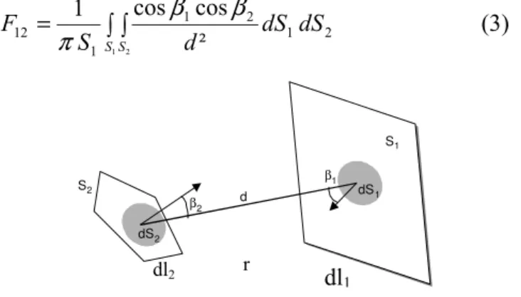
2.2 Computation of view factors

The view factor F12 is the fraction of radiative flux,

emitted from an elemental surface dS1, and directly

received (without any reflexion or transmission) by an other elemental surface dS2.

2 1 2 1 1 12 1 2 ² cos cos 1 dS dS d S F S S ∫ ∫ = β β π (3)

Fig. 1. View factor definition.

Many numerical methods exist to compute view factors. One of them is the contour method [5], based on the theorem of Stokes to transform the integrals of surface of the equation (3), in curvilinear integrals: ∫ ∫ ⋅ = 1 2 1 2 1 12 ln 1 C C dl dl r S F π (3)

Then integrals are computed with the Gauss method. Different ways exist to evaluate the radiative heat flux absorption. One of them is the Beer-Lambert model.

2.3 The Beer-Lambert law

The main idea of this law is that the radiative flux is absorbed in the medium according to a decreasing exponential: ) exp( ) (x q₀ x q_λ = _λ −σ_aλ (4)

where qλ(x) = monochromatic radiative flux at the

location x, q0λ = incident monochromatic radiative

flux, σaλ = spectral absorption coefficient of PET.

Although this law avoids long computation times, it is reserved to non scattering cold media [6]. This law is integrated over the frequency in the spectral band [0.2 - 10µm].

3 INFRARED OVEN OPTIMIZATION

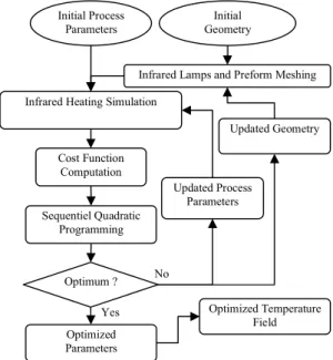
The analytical computation of irradiance is coupled to an optimization method, to automatically modify

S₂ β2 d dS₂ S₁ β1 dS₁ dl2 _dl 1 r

oven geometric parameters at each iteration, as shown in figure 2. The problem being non linear, continuous, and constrained, an adapted Sequential Quadratic Programming method is developed using Matlab® [7].

Fig. 2. Heat transfer simulation / optimization coupling. 3.1 Cost function

The optimisation objective is mathematically represented by a cost function F to minimize, function of oven design parameters X. We propose to establish the function (5) related to temperature uniformity at the surface of the preform, and to a desired mean value of temperature.

OBJ OBJ T T X T X X F( )= 0.5 (₀ )+0.5 ( ( )− ) σ σ ₍₅₎ 2 , ) ( 1 ) ( = ∑n − j i ij T T n X with σ (6)

where T(X) = mean temperature computed at each iteration, TOBJ = desired mean temperature, σ(X) =

standard deviation of computed temperatures at each iteration, σ0 = standard deviation of computed

temperatures with initial conditions, n = number of preform surface elements. This function permits to obtain not only a uniform temperature field, but a desired mean value of temperature too.

3.2 Parameters

Both process and geometric parameters can be included in the optimisation. In this study, we focus

on geometry only. Parameters concerned are: distances between IR lamps and the preform (X1, X2,

X6, Y7), and the distance between lamps (E), as

shown in figure 3.

Fig. 3. Adopted configuration / parameters notation. 3.3 Constraints

Geometric parameters are bounded. For example the distance between lamps must be greater than 20 mm, in order not to damage IR lamps. These constraints can be expressed as inequality relations between several parameters.

4 APPLICATION

The method developed is used to optimize the geometry of an oven constituted of seven halogen lamps 1 kW, according to the cost function (5). The objective mean value of temperature is 110 °C. Dimensions of the PET preform are: 110 mm height, 25 mm diameter, 2 mm thickness. It is meshed into 4600 elements.

Fig. 4. Preform and lamp meshes.

Infrared Heating Simulation

Cost Function Computation Sequentiel Quadratic Programming Optimum ? Initial Process Parameters Initial Geometry

Infrared Lamps and Preform Meshing

Updated Process Parameters Updated Geometry Optimized Parameters Optimized Temperature Field No Yes E x2 y7 E x1 x6

The value of the convective coefficient, applied to preform surface during heating stage, is equal to 30 W/(m².K). Results are reported in table 1.

Table1. Initial and final parameters Parameters

(mm) X1 X2 X6 Y7 E

Initial 20 20 20 130 20

Final 20 30 30 129 19

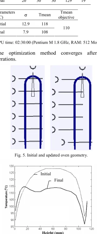
CPU time: 02:30:00 (Pentium M 1.8 GHz, RAM: 512 Mo). The optimization method converges after 26 iterations.

Fig. 5. Initial and updated oven geometry.

Fig. 6. Front surface temperature distribution after 15 s heating, computed with Termoray. Initial and updated oven geometry.

As shown in figure 6, a more homogeneous temperature distribution over the preform surface is obtained using updated oven geometry, even after 15 s heating. The gain of uniformity is equal to 38%.

5 CONCLUSIONS

A complete numerical model of the heating stage has been developed. Using a control-volume software, the 3D heat balance equation is solved with convective and radiative boundary conditions. The radiative flux absorption is computed according to the Beer-Lambert law. Concerning the optimization, the SQP algorithm coupled with the thermal solver permits to design optimally ovens geometry, in order to increase the surface temperature uniformity. Actually the optimal temperature field may not be uniform. That’s why it is crucial to determinate by a numerical or an experimental way, the real optimal temperature field. Then the goal will be to optimize either the preform mean temperature, but the temperature profile.

The others tasks for the future work will consist in taking into account lamps powers in optimization, and to define a new cost function including the process efficacy.

REFERENCES

1. H.-X. Huang, Temperature profiles within reheated preform in stretch blow molding, In: SPE Annual Technical Conference - ANTEC’05, (2005).

2. S. Monteix, F.M. Schmidt and Y. Le Maoult, Experimental Study and Numerical Simulation of Preform or Sheet Exposed to Infrared Radiative Heating, In: Journal of Materials Processing Technology.119, (2001) 90-97.

3. C. Champin, 3D Finite Element Modelling of the Strech Blow Moulding Process, In: 8th ESAFORM conference on material forming, 2005.

4. K.T. Nguyen, An inverse method for estimation of the initial temperature profile and its evolution in polymer processing, In: International Journal of Heat and Mass Transfer.42 (1999) 1969-1978

5. E.M. Sparow, A New and Simpler Formulation for Radiative Angle Factors, In: Journal of Heat Transfer.85, (1963) 81-88,

6. M. Modest, Radiative Heat Transfer, McGraw-Hill, Inc (1993).

7. Optimization Toolbox For Use With Matlab, The MathWorks (2002), User’s Guide, Version2.

Parameters (°C) σ Tmean Tmean objective Initial 12.9 118 Final 7.9 108 110 Initial Final Height (mm)