ANALYTIC SURGERY
AND
ANALYTIC TORSION
Andrew Hassell
B. Sc. (Hons), Australian National University, 1989
Submitted to the Department of Mathematics in partial fulfillment of
the requirements for the degree of
Doctor of Philosophy
at the
Massachusetts Institute of Technology
May 1994
@1994 Massachusetts Institute of Technology All rights reserved
Signature of Author
..
-
,
Department of Mathematics April 20, 1994 Certified by . , --Richard Melrose Professor of Mathematics Thesis Advisor Accepted by J>,rAY1L V o Science.i .
14'
;
AUG 1 1 1994 lCavi u v caI Professor of Mathematics Director of Graduate Studies3
Analytic surgery and analytic torsion
Andrew Hassell
Submitted to the Department of Mathematics in partial fulfillment of the requirements for the
degree of Doctor of Philosophy
at the Massachusetts Institute of Technology
Abstract
Let (M, h) be a compact manifold in which H is an embedded hypersurface which separates M into two pieces M+ and M_. If h is a metric on M and x is a defining function for H consider the family of metrics
dx2
gE = X22-
+-h
+ 2 +hwhere e > 0 is a parameter. The limiting metric, go, is an exact b-metric on the disjoint union M = M+ U M_, i.e. it gives M+ asymptotically cylindrical ends with cross-section H. We investigate the behaviour of the analytic torsion of the Laplacian on forms with values in a flat bundle, with respect to the family of metrics
g,. We find a surgery formula for the analytic torsion in terms of the 'b'-analytic
torsion on M±. By comparing this to the surgery formula for Reidemeister torsion, we obtain a new proof of the Cheeger-Miiller theorem asserting the equality of analytic and Reidemeister torsion for closed manifolds, and compute the difference between b-analytic and Reidemeister torsion on manifolds with cylindrical ends. We also present a glueing formula for the eta invariant of the Dirac operator on an odd dimensional spin manifold M. This generalizes a result of Mazzeo and Melrose, who obtained a similar glueing formula under the assumption that the induced
Dirac operator 3H on H is invertible. In both cases there is an 'extra' term in the glueing formula coming from the long time asymptotics of the heat kernel. The
term can be expressed in terms of a one dimensional Laplacian associated to the null space of the Laplacian on M. This operator is determined by scattering data on M at zero energy, and controls the leading behaviour of small eigenvalues as
e 0.
Thesis Supervisor: Richard Melrose Title: Professor of Mathematics
To my parents, Jenny and Cleve
7
ACKNOWLEDGEMENTS
I would like to express my deep gratitude to my advisor Richard Melrose for suggesting a terrific thesis problem, for sharing with me his mathematical insight, and for his encouragement. His influence is evident on every page. I am also grateful to Rafe Mazzeo for sharing his ideas with me. As noted below, this thesis is in part joint work with both of them.
I am indebted to many other graduate students at MIT, present and former, for friendship and mathematical discussions, particularly Tanya Christiansen, Alan Blair, Richard Stone and Mark Joshi. To all my other friends here, I wish to express my appreciation for their support.
The financial support of the Australian-American Educational Foundation and the Alfred P. Sloan Foundation is gratefully acknowledged.
This work is dedicated to my parents in appreciation for their constant love and encouragement.
DECLARATION
Some of this thesis is joint work. The single and double logarithmic spaces were developed jointly with Richard Melrose and Rafe Mazzeo. Much of chapters 2, 3 and 4 is due in part to Richard Melrose, and several other ideas in the thesis were influenced or suggested by him. It is intended to publish chapters one through nine in a joint paper with Mazzeo and Melrose. Otherwise, except where noted in the text, the work described here is my own.
CONTENTS
Chapter 1. Introduction ...
1.1. Analytic surgery ... 1.2. Eta invariant and analytic torsion . 1.3. Statement of Results1.4. Outline of the proof .
..
. 1313
..
. 14..
. 15..
. 17Chapter 2. Manifolds with corners, blowups and b-fibrations 20 2.1. Manifolds with corners 2.2. Blowups . . . . 2.3. Operations on conormal functions . 2.4. Two Blowup Lemmas .. . . . 2.5. Logarithmic blow up 2.6. Total boundary blow up .
Chapter 3. The Single Space . . ..
3.1. Definition .... 3.2. Densities ... 3.3. Lift of V,(X) . . . . 3.4. Models ....
20
...
... . . 21 . . . . 22 . . . 24 ... . . 27 .28 ... . . . 31 ... . . . ... . . . . 31 ... . . . 32 ... . . . ... . . . . 33 ... . . . ... . . . . 37Chapter 4. The double space and the pseudodifferential calculus . . 41
4.1. Preliminary remarks . . . .. . . . . 41
4.2. Logarithmic Double space .. . .. . . . . .. . . . 41
4.3. Densities ... ... 43
4.4. Logarithmic Surgery Pseudodifferential Operators . . . 44
4.5. Action on Distributions .. . . .. . . . 45
4.6. The Triple Space . . . .. . . . 46
4.7. Compositon and the Residual Space .. . . . .. . . . . 46
4.8. Symbol Map . . . .. . . . 48
4.9. Model Operators.
...
. . . 49
4.10. Neumann Series for Residual Operators ... . . ... .. . . 50
4.11. Composition of small calculus with residual calculus . . .. . .. . 51
Chapter 5. One dimensional surgery resolvent . 5.1. Scaling property. 5.2. Scattering Matrix ... 5.3. Properties at the boundary . . . . 5.4. Eigenvalues ... 5.5. Heat kernel and large
Izi
asymptotics of . 5.6. Determinant and eta invariant. .. . . . 53 ... . . . . 53 ....
54
...
54
...
55
...
55
...
57
11 . . . . . . . . . . . . . . . . . . . . . . . .Chapter 6. Resolvent with scaled spectral parameter
6.1. Preliminaries ...6.2. Terms of order (ias)-l ... 6.3. Terms of order (ias E) .
6.4. Terms of order (ias E).
6.5. Compatibility with the symbol . . . .. . 6.6. From parametrix to resolvent .
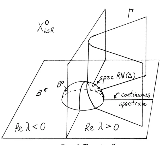
6.7. Near the discrete spectrum of RN(A). 6.8. In the presence of L2 null space . 6.9. Very small eigenvalues .
Chapter 7. Full Resolvent ... 7.1. Resolvent spaces ...
7.2. Operator Calculus ... 7.3. Full Parametrix ...
7.4. Full Parametrix to Full Resolvent .
... ...
60
... 60
... ... 63 ... ... 64 ... ... 67 ... ... 67 ... ... 67 ... ... 68... ...
70
... ...
71
... ... 73 ... ... 73... ...
75
75... ...
78
Chapter
8.
Heat
Kernel
... ...
... .. .80
8.1. The Heat Space and the Heat-Resolvent Space .. ... . . . . 80
8.2. Contour spaces. . . ... . . . .... 81
8.3. Behaviour as t - . ... . . . . .. . . . 84
8.4. Very small eigenvalues .. . . . .. . . . .. .. . . . . 87
8.5. Full Heat Kernel. .. ... . . . 88
Chapter 9. Limit of Eta Invariant 9.1. Eta invariant. 9.2. The diagonal of the Logarithmic heat space 9.3. Asymptotic expansion of iq as e - 0 . ... . . . 89 . ... . . . 89 . ... . . . 89 . ... . . . 90 .
Chapter 10. A Hodge Mayer-Vietoris cohomology sequence 10.1. Mayer-Vietoris sequence . . . ... 10.2. b-Hodge theory ... 10.3. Surgery Hodge theory ...
Chapter 11. Analytic Torsion and Reidemeister torsion . . .
11.1. Analytic torsion. 11.2. Surgery formula for analytic torsion. 11.3. Reidemeister torsion .. . . . .. . . . .. 11.4. Cheeger-Miiller Theorem. . 93 .. . 93 . . 93 . 94 . .. 97 .. . . 97 . . 99 . . . 102 . . . 104Chapter 1. Introduction
1.1. Analytic surgery.In this thesis, we continue the study of analytic surgery initiated in [15]. By "analytic surgery" we mean a singular deformation of a Riemannian metric on a closed manifold M that models the cutting of M along a hypersurface H (possibly disconnected), forming a manifold with boundary M ("surgery"). For simplicity we assume that H separates M; thus M is the disjoint union of two manifolds with boundary M±. We consider a specific deformation which degenerates to a complete metric on M of the form dx2 /x2 + h, where x is a boundary defining function for H (that is, > 0, H = {x = 0} and dxz 0 on H) and h is a smooth metric on M. This form of metric on a manifold with boundary, called an "exact b-metric" and studied in some detail in [17], gives M asymptotically cylindrical ends, with log x approximately arc length along the end. Specifically, we consider a family of the form
dx2
ge - 2 e2 + h;
this is a smooth metric on M for every e > 0, which develops a long neck of length 2 log 1/e + 0(1) -- oo as e -- 0 and whose singular limit is manifestly an exact b-metric on M.
Similar deformations, usually phrased in terms of a family of manifolds which have a long cylindrical neck across H with length I - oo, have been studied by several authors. There are two main reasons for interest in this procedure. One is to understand the behaviour of geometric or topological invariants such as the index of a Dirac operator, eta invariant or analytic torsion under surgery, as in [4], [6], [10], and [8]. The other is to analyse the behaviour of the spectrum of operators (such as the Laplacian) under the transition from closed manifold to complete manifold. In Mazzeo and Melrose's paper [15] and the present thesis, both questions are investigated. Of course these two problems are closely related. In this thesis glueing formulae for the eta invariant and analytic torsion under surgery are presented, but these are obtained by studying the full resolvent family of generalized Laplacians under surgery, including the analysis of accumulation of eigenvalues at the bottom of the continuous spectrum of A0.
Closely related are the papers of McDonald [16] and Seeley and Singer [28], who studied metric degeneration to incomplete conic metrics, and Ji [13], who studied degeneration of Riemann surfaces to surfaces with hyperbolic cusps. It should be remarked that the approach of McDonald inspired [15] and the present work.
There are two motivations for the choice of a "cylindrical ends" metric for M. One is that Atiyah, Patodi and Singer obtained their well-known global boundary condition for the Dirac operator on a manifold with boundary in [1] heuristically by considering a cylindrical end attached to the boundary. The other is that Richard Melrose has presented a detailed analysis of the Laplacian associated to an exact b-metric in [17], as well as a proof of the APS index theorem in the 'b' context. It
would also be interesting to study metric degeneration to other types of complete metrics, such as metrics with asymptotically hyperbolic or Euclidean ends.
1.2. Eta invariant and analytic torsion.
The eta invariant was introduced by Atiyah-Patodi-Singer in [1] as the boundary term in the index formula for the Dirac operator on a manifold with boundary. (For a discussion of Dirac operators see [17], [2] or [14].) It is a spectral invariant, given by the analytic continuation of the eta function 1r(s) = A•.xO0Espec sgn A
AI
- tos = 0. Alternatively, it has a formula in terms of the heat kernel:
(1.1) (o) =
j
ti Tr (e-t2) dtthis is the formula we will exploit here. In order to generalize index formulae, it is of interest to extend the definition of eta to operators which have continuous spectrum. For manifolds with boundary and a b-metric, the heat kernel is no longer trace class but the b-eta invariant was defined in [17] as in (1.1) with Tr replaced by the 'b-Trace' (see section 2.3); it is a natural regularization of the integral. This thesis is intended to illustrate the relation between these two definitions, and to throw light on the index theorem for a manifold with corners carrying a b-metric.
The analytic torsion T is an invariant of a flat bundle E over a Riemannian manifold M introduced by Ray and Singer. It is defined by formal analogy with a formula for Reidemeister torsion, or R-torsion, denoted r, on a simplicial complex. It is given by
log T(Mn, g, E)
=2 (-1)q+lq log det
Aq-
(-l)qq(
(q)(0),
q=0 q=o
where q is the zeta function for A', the Laplacian on q-forms with values in E, projected off the zero eigenspace:
(1.2)
()
=
Tr t es .AEspec rs) 2
Ado
Since for finite rank operators '(0) = - log A, this is a natural regularization of the log determinant of an operator. Ray and Singer showed that T(M, g) has the same formal properties as R-torsion and conjectured that these two torsions are equal. This was proved several years later by Cheeger and Miiller independently in [7] and [22]. In recent years, several more proofs and generalizations of this result have appeared. Vishik [29], [30] has established the relationship between analytic torsion, defined using classical boundary conditions, and R-torsion on manifolds with corners. Burghelea-Friedlander-Kappeler [5] obtained a new proof using Wit-ten's deformation of the de Rham complex via a Morse function. Miiller in [23] extended the result to bundles E assuming only that the determinant bundle det E
1.3. STATEMENT OF RESULTS 15
is flat. Bismut-Zhang [3] proved a further generalization when the bundle E is not necessarily flat; the difference log(T/r) is given by the integral of a local 'anomaly'. It is interesting to compare Vishik's formula for T/r on a manifold with boundary with Corollary 1.7; in both cases the ratio depends on the Euler characteristic of the boundary.
As with the eta invariant, one would like to extend the definition of the log determinant to operators which have continuous spectrum. We do this for the Laplacian on forms, as in [17, chapter 9], by defining the b-C function, replacing Tr with b-Tr in (1.2). Then the b-analytic torsion is defined using these regularized log determinants. In this thesis, we study the questions: how is the b-analytic torsion related to the torsion on a closed manifold? How is b-analytic torsion related to Reidemeister torsion? Most of the proofs of the equality of T and r are indirect: one establishes that T and r have the same glueing formula under surgery and uses this to compare the two torsions of an arbitrary manifold to the sphere Sn for which the result is known. Here we derive a glueing formula for T under analytic surgery, which by comparing to the analogous formula for R-torsion, enables us to compute the ratio of R-torsion and b-analytic torsion on manifolds with boundary.
1.3. Statement of Results.
Let us first recall the main results from Mazzeo and Melrose's paper [15], hence-forth referred to as 'Mazzeo-Melrose'. There the same situation, for the eta invari-ant, was studied, under the assumption that the induced Dirac operator on H is invertible. A "surgery double space" and "surgery heat space" were introduced as spaces to carry the Schwartz kernels of (A - A2) -' and e-t ' uniformly as e - 0. They are blown up versions of M2 x [0, eo], and M2 x [0, oolt x [0, eo], which resolve the singularities of the space of vector fields V, associated with the family g,. The resolvent and heat kernel were shown to be polyhomogeneous conormal half densi-ties on these spaces and their leading asymptotics (model operators) at e = 0 were identified. It was shown that the projector II, onto eigenfunctions with eigenvalue going to zero with e is a finite rank, smoothing operator. They showed:
THEOREM. (Mazzeo-Melrose) Let (e) be the signature of nI. If the induced Dirac
operator on H is invertible, then the eta invariant of 3 satisfies
,I(a,)
-(e) =
'qb(3M+)+
b(3M) +
er(e) +
log
r2(),
with ri E C°([O, eo]).
Douglas and Wojciechowski obtain a similar result in [10].
Unfortunately the assumption on invertibility of the operator at H excludes many interesting cases, including the surgery limit of analytic torsion when H*(H, E) does not vanish. A principal goal of this thesis is to extend to machinery of Mazzeo-Melrose to deal with the case when the operator on H has null space. To do this the constructions in Mazzeo-Melrose must be modified. One reason for this is that when dH has null space the heat kernel no longer has uniform exponential decay, as it does (up to finite rank) in [15]. One must understand the leading behaviour of
the heat kernel as t -, oo to calculate the integrals (1.1) and (1.2), which amounts to understanding the leading behaviour of the resolvent as A - 0. This means, in contrast with Mazzeo-Melrose, that one must understand the resolvent down to the bottom of the continuous spectrum of Ao, and in particular, the leading behaviour of small eigenvalues, that is, those going to zero with e. To cope with this we perform further blowups on the spaces of Mazzeo-Melrose, to resolve singularities in the kernel that form as we approach A = e = 0. We introduce the "logarithmic double space" X2 and "logarithmic heat space" XHs; the names are due to the application of "logarithmic blowup" (see section 2.5) to each face of the surgery double space. Then we get analogues of the results above. Introduce the function iase = 1/sinh-'(1/e) ("inverse arc-sinh"), which is the reciprocal of the growth rate of the volume of M. It goes to zero with E, but only logarithmically. For the resolvent we scale A by writing A = (ias e)z to capture the behaviour of small eigenvalues. Thus when e = 0, A = 0 for all z.
THEOREM 1.1. The resolvent (A - (ias e)2z2)' is a meromorphic family of conor-mal half densities on X x C, (ias e)-1x smooth up to the boundary of XL2,. The poles z(e) satisfy lim,.0 z(e) = 0 or zj, where {z2} are the eigenvalues of a one dimensional Laplacian RN(A) on [-1, 11 with boundary conditions determined by
scattering data on M.
We prove this in chapter 6. Indeed we extend the result in chapter 7 to the full resolvent which includes the resolvent away from the spectrum at e = 0 as in Mazzeo-Melrose. From this we get the heat kernel via a contour integral. With II, now denoting the (finite rank) projection onto eigenfunctions with eigenvalue A2(E) = o((ias e)2), we have
THEOREM 1.2. On XLHS the heat kernel projected off zero modes, e- t- - II, is
t-,/ 2 times a smooth half-density for t near zero and is smooth up to t = oo. II itself is smooth except possibly up to t = oo.
In both cases we know the top terms at each boundary face. In principle one can calculate the Taylor series at every face at e = 0 to arbitrary order.
From this we read off the behaviour of the eta invariant.
THEOREM 1.3. Let rlfd(e) be the signature of IIE. Then
(3e) - fd(e) = 7b(M+) + 7b(3M_ ) +
i7(RN(3))
+ (ias e)r(ias e), where r is smooth.Thus we get, in comparison with the case when aH is invertible, an extra contri-bution ij(RN(3)) coming from the small eigenvalues.
For analytic torsion, we measure torsion relative to a fixed set of cohomology classes. If A' is an orthonormal basis of the surgery Hodge cohomology group
1.4. OUTLINE OF THE PROOF
THEOREM 1.4. T(M,p i) is given by
log T(M, pi') = log bT(M+, go) + log bT(M_, go) + 2 (- 1)+1 q log det RN(aq ).
q=O
Comparing to the surgery formula for R-torsion, we get
THEOREM 1.5. The difference log T - log r obeys the surgery formula
T(M, g)
bT(M+,go)
bT(M_ , go) +
log
7(M, g)= log
(M+, go) +log
r(M-, go)
+2
XE(H)log2.
Applying Cheeger's argument from [7], we obtainCOROLLARY 1.6. (Cheeger-Miiller Theorem) For a closed manifold with flat unitary
bundle E and metric g,
T(M,g)= (M, g).
COROLLARY 1.7. For a manifold with boundary N, with flat unitary bundle E and
exact b-metric g, we have
bT(N,g) = 2-XE(°N)/4r(N,g).
1.4. Outline of the proof.
We may take as a starting point for the considerations in this thesis the fact that the eigenfunctions whose eigenvalues go to zero under surgery are not smooth on the "single space" X, of Mazzeo-Melrose; indeed they are not continuous. One can easily see this by looking at the example of surgery on an interval, or a circle. Then the eigenfunctions of A, look like e2lrikr /
L, where r = sinh-1 (x/e) is arclength and 2L, = length of g,. Then on the surgery space X, = [M x [0, eo],; H x 1}] of Mazzeo-Melrose, this eigenfunction is equal to 1 on the surgery front face BS and (-l)k on the b-boundary Bbb. The oscillations disappear into the corner B,, n Bbb. To rectify this situation we replace, in chapter 3, the single space by a new space, XLs, on which the scaled distance r/L, is a smooth function. XL, is a blown up version of X, involving the operation of logarithmic blowup described in section 2.5. We then modify, in a methodical way, all constructions in Mazzeo-Melrose to reflect this change. The Lie Algebra V. of Mazzeo-Melrose is lifted to VL, on XLS; properties of VL, including its normal operators, are discussed in chapter 3.
We microlocalize the Lie Algebra VLS according to the general principles set forth in [20]. This means we need the following things. First, we need a double space X2 to carry Schwartz kernels of "logarithmic surgery pseudodifferential operators", or Ls-tbdos, with diagonal submanifold ALs such that kernels of VL-differential oper-ators are given precisely by all distributions on XL.s supported on ALs with poly-nomial symbols. By replacing polypoly-nomial symbols with arbitrary classical symbols, we obtain the "small calculus". Second, the double space should have a natural map down to the single space XLS which is a b-fibration (see chapter 2) so that kernels 17
can act on distributions on XL. Third, there should be a triple space XLs with a b-fibration down to XLs so that composition of Ls-4dos can be defined. Finally, the normal operators on VLS should extend to "model operator maps" on Ls-4dos given by restriction of the kernel to faces at e = 0. Geometric lemmas to help construct these spaces are given in the second half of chapter 2 and the surgery pseudodifferential calculus is set up in chapter 4.
In view of the Pushforward theorem of [19], discussed here in section 2.3, the fact that we have b-fibrations X3, - X XL means that we can work in the class of polyhomogeneous conormal functions throughout. This has the virtue of almost eliminating estimates from the thesis, as we easily read off the decay rate of functions from the index set specifying its (poly)homogeneities. This comes at the cost of fairly complicated spaces and geometric machinery but we are able to obtain detailed information about the resolvent, heat kernel and small eigenvalues with this method. Because of the logarithmic blowups we are able to work with "natural" index sets (see section 4.7) and show that our final objects - resolvent, heat kernel, eta invariant and analytic torsion - are smooth in the blow-up coordinates.
In chapter 5 we analyse the model problem coming from the reduced normal operator in chapter 3. This is a "new" model operator, not appearing in
Mazzeo-Melrose, and Proposition 3.8 indicates that the eigenvalues of this model control the leading behaviour of small eigenvalues of A,. We show that this model is a nice half density on the double space; this indicates that XLS is the "correct" space to use, and we use the model heavily in chapter 6 in the construction for the general resolvent.
In chapters 6 and 7 we make a start on the problem of understanding (A- A2)-' when A approaches the spectrum. We construct the resolvent near the bottom of the
continuous spectrum, 0. We blow up at A = 0, introducing the rescaled parameter z = A sinh - 1(1/e) which captures the scaling of small eigenvalues. To construct the parametrix we need to solve not only the symbol at the diagonal singularity but also solve a finite number of model problems at each boundary face. Compatibility conditions at the intersections of faces give boundary conditions for these model operators, which enable them to be solved uniquely; the interaction between the models on various faces and of different orders is fairly complicated.
In principle, once we have the resolvent we can construct any function of the Laplacian by functional calculus. We construct the heat kernel in this way in chapter 8. More precisely, we obtain it by performing the contour integral
(1.3) t' =- 1 e-t2(A - A2
-2AdA.
)Then we obtain the eta invariant and analytic torsion by performing the integrals (1.1) and (1.2). This integral is really a pushforward, since the integrand lives on a blown-up version of its space of parameters. We construct spaces so that the integral becomes a pushforward under a b-fibration. This allows us to conclude that the result is polyhomogeneous, and an extra argument shows that it is actually smooth. We compute the leading terms of the heat kernel at t = oo.
1.4. OUTLINE OF THE PROOF 19
In chapters 9, 10 and 11 we then make three applications of this machinery. The first is a surgery formula for the eta invariant, Theorem 1.3. The second, in chapter 10, is a Hodge version of the Mayer-Vietoris sequence in cohomology for the triple (M, M+, M_); we also obtain a spectral gap result between the eigenforms corresponding to cohomology on M and the other eigenforms. In chapter 11 we compute the surgery limit of analytic torsion and R-torsion (using results of chapter
10) and compare them, obtaining theorems 4 and 5. The first corollary follow then follows from Cheeger's well known approach [7] to proving the equality of analytic
Here we present material on the geometry of manifolds with corners that we need in this thesis. We will assume familiarity with [19], but we also recall a fair amount of this material in the first three subchapters, although sometimes with a different presentation. We then go on to describe two "new" blowup operations which we use heavily in the sequel, logarithmic blowup and total boundary blowup.
2.1. Manifolds with corners.
We refer to [19] for a discussion of manifolds with corners, tangent space, b-maps, and b-fibrations. Let us recall here that the set of boundary hypersurfaces of a manifold with corners X is denoted M1(X), and the set of proper faces, that is, all faces excluding X itself, is denoted M'(X). A boundary defining function p for a boundary hypersurface H of a manifold with corners Y is a smooth nonnegative function on Y such that p = 0 on H, dp # 0 on H. A smooth map between manifolds with corners f: X --. Y is an (interior) b-map if for every boundary defining function PH for Y,
(2.1) fPH = a pe(GH)
GEMI(X)
for some nonzero smooth function a and (uniquely determined) collection of natural numbers ef(G, H), called the boundary exponents of f.
We will be especially concerned with special b-maps called b-fibrations; the map
f above is a b-fibration if the map f on the b-tangent bundle is surjective on each fibre, and the image of each boundary hypersurface in X is either Y or one boundary hypersurface H C Y. (This definition is different from, but equivalent to, the definition given in [19].) b-fibrations have good mapping properties on M'(X); the image of any face F E M'(X) is a face in M'(Y), and frF is a b-fibration onto
its image.
p-submanifolds There are various possible definitions of a submanifold of a manifold with corners; we will use a very strong definition. A subset S C Y is a p-submanifold if locally, in some coordinate system l,... , y, *... Y-k with x' > 0, yj E (-6,6 ), S is given by the vanishing of some of them: S = {x = . .
Ye = ' -- = Yj, =
0}.
Then, if S is connected, S has a tubular neighbourhood which is a bundle over S, the fibre being a neighbourhood of 0 E R-r x Rl"'-' -m. We say S is an interior p-submanifold if 1' = 0 in the definition above. If f is as above and S is an interior p-submanifold, then f-1 S is a p-submanifold; if S is not interior, then in general f -'S is a union of p-submanifolds of X. This is clear in local coordinates. Choose coordinates in Y such that S has the form above; then it is possible to choose coordinates xl,... l,... Yn-k, with xi > 0, y E (-6, 6)locally in X so that locally f has the form
f(Xi,..
XkY1,.. Yn-k) =(
I
Xr,
II
rY1,.--dYn'-k)
rEI rEI,
2.2. BLOWUPS
Then f-IS is a union of p-submanifolds r,, = = Yjl = ... yjm = or'" with ri E Ii.
Degrees and density bundles We will find it convenient to use the notion of the "degree" of a boundary hypersurface H of a manifold with corners X. This is simply an assignment of an integer, d(H), to H. Informally this is supposed to represent the order of growth of densities allowed at H. If each boundary hypersurface of X has been assigned a degree, the degree density bundle is defined by
Q(X)
I
p-d(H)Q (X)=
P-d(H)-1Q(X)~ PHHEM1(X) HEM1(X)
where PH denotes a boundary defining function for H. Observe that b-densities have the pleasant property that dPH/pH is a canonical factor at H, so dividing by
IdPH/PHI gives a canonical restriction C°°(Qfb(X)) -, C°°(Qb(X)). With general
D-densities, restriction defined by division by IdpH/P (H)+ I depends on the choice
of boundary defining function. However, in this thesis we will have a canonical total boundary defining function (product over M1(X) of boundary defining
func-tions) R for many of our spaces. In this case division by IR-d(H)dpH/PHI gives a canonical restriction C°°(QD(X)) -, C°(QD(H)), where the degrees of boundary
hypersurfaces H n K (K E M
1(X)) of H are defined by d(H
n
K) = d(K) - d(H).
2.2. Blowups.
If S C Y is a p-submanifold, the blowup of Y at S, denoted [Y; S], is a manifold with corners , given as a point set by (Y \ S) U (SN+ S) and with C° ° structure the unique minimal structure such that functions on Y lifted to S, and polar coordinates at S, are smooth. (SN+ S is the inward-pointing spherical normal bundle to S.)
There is a unique smooth map [Y; S] - Y extending the identity on Y \ S, called the blowdown map. The lift of a p-submanifold T C Y to [Y; S] is defined if (i)
T C S, in which case the lift is defined to be the inverse image of T under the
blowdown map or (ii) T \ S is dense in T, in which case the lift is defined as the closure of T \ S in [Y; S].
We will often perform sequences of several blowups to create new spaces in this thesis, and it will be important to know when one can exchange the order of blowup. Here we present two easy results of this nature.
LEMMA 2.1. If S, T are p-submanifolds of Y and either (i) S and T are transverse
or (ii) T C S then [Y; S; T] = [Y; T; S].
PROOF: The proof of (i) is immediate because there NS and NT are independent and so the blowups occur in two disjoint sets of variables.
To prove (ii), it is sufficient to consider the case T = {0 O, S= x Rm,
=
R x R", k > 1, n > m. Define R = k X2 + l 2 and Rs = + 2+
E=m+i
y2. In both [Y; S; T] and [Y; T; S] the lift of T and S have boundary defining functions (the lift of) RT and Rs respectively, and a superset of coordinates on the lift of T is given by xi/(zi + RT), yj/(Yi + RT) for i,j > 1 and on the lift ofS by xi/(xi + Rs), yj/(yj + Rs) for i > I+ 1,j > m+ 1 on both spaces. This means
that the identity map on Y \ S extends to a smooth map [Y; S; T] - [Y; T; S in both directions. Each extension is therefore a canonical diffeomorphism. I
2.3. Operations on conormal functions.
The principal function spaces used in this thesis are spaces of polyhomogeneous conormal functions, conormal either at a boundary hypersurface, as described in [191, or an interior p-submanifold (eg, the diagonal). For such spaces we have the Pullback and Pushforward theorems, allowing us to pull back and integrate whilst preserving polyhomogeneity. These theorems are discussed in [19]; here we recast them in the language of D-densities and also discuss the interior p-submanifold case. Let f: X - Y be a b-fibration between manifolds with corners with degrees and
let ex(G) = d(G) - d(H) for G E M1(X) if f(G) = H E M1(Y), ex(G) = d(G) if
f(G) = Y.
THEOREM 2.2. (Pullback theorem) f induces a pullback map on functions
f*: Ag(Y) -
Af
(X)
where f#()(G)
= 0 if f(G) = Y, f#()(G)
= {(e(G,H)z + q,k) I (z,k) E
J(H),q e N} if f(G) = H.
THEOREM 2.3. (Pushforward theorem) If Re/C(G) > d(G) for all G such that
f(G) = Y, then the pushforward by f, that is, integration, of smooth compactly supported densities extends to a map
f#:
A h(X;
D(X))
-
A#(-Kex)(y;
,(y))where f#(IC)(H) = { (z, k) 3 G1... Gk mapping to H and P1 ... Pk such that
(z/e(Gi, H),pi) E
AC(Gi)
and p = pi +
* *
+ Pk + (k - 1)}.
The coefficients of the pullback f* h at a boundary defining function G in the first theorem are given by pullbacks of restrictions of h to f(G). Under pushforward, if the inverse image of H E M1(Y) is just one boundary hypersurface G then the
coefficients of flu are the pushforwards of the restrictions of u to G under frG, using consistent boundary defining functions on X and Y to restrict. If the inverse image of H is more than one boundary hypersurface of X then it is a messy business to specify in general how the coefficients of u and f.u are related. Let us give a example to illustrate a fairly simple case, and which will be sufficient for the computations in this thesis.
EXAMPLE 2.4. Let C be the COo index family for X, let f: X - Y be a b-fibration
and suppose H E M1(Y) and exactly two boundary hypersurfaces G1, G2 map to
H, with ef(Gi,H) = 1 and ex(Gi) = 0. Let u E A'hg (X; QD(X)). The index set
for flu at H is {(n, O0), (n, 1)
I
n E N}. Let p be a boundary defining function for the2.3. OPERATIONS ON CONORMAL FUNCTIONS
near int G1 G2. Use these boundary defining functions to restrict densities to
these boundaries. Then
u - (logpao,l + ao,o + O(plog p)) d(H)+1
where a,l = (frG nG2)*(urtGnG2) and, with +)(x) a cutoff function near 0, equal to
1 near 0 and vanishing for x > 1,
a0,0 = lim [(fri
)*
((1 - )( ) GI) + (frG2)*((1- i)( ) utG) + 2 log6 a o,].These pushforwards are regularized integrals; the pushforward of u rG does not exist because u is not integrable up to the boundary.
More generally, if f: X -- Y is a b-fibration, G is a boundary hypersurface of X with boundary defining function p, and u is a b-density on X which is integrable at all boundary hypersurfaces except possibly G, then the limit
lim f# ((1 - X[o,6])(p) ) - log 6(ftG)#(U rG)
610
exists and is denoted b-f u, or b-f u if the dependence on p needs emphasizing. The regularized integral depends on p through the section dp of N*G; we have
bp -
u -
-
(f ra)#(ur
log
lg (dPi
If the integral is formally computing the trace of an operator, then the regularized integral is denoted b-Trdp. In the case of the regularized integral defining the b-eta invariant on Mi, the integrand at the boundary vanishes pointwise after taking the pointwise trace, and so the b-eta invariant is independent of the choice of boundary defining function. For the b-zeta function, the integrand at the boundary is constant in t, after taking pointwise trace and summing in q, and this implies that the b-zeta function itself is also independent of the choice of boundary defining function. Hence both these quantities are completely well defined.
The pushforward theorem also holds if we allow our densities on X to have interior singularities along a p-submanifold S transverse to all boundary hypersurfaces of X and to f. We denote such a space I
A
phg (X; QD(X); S) if the conormal order atS is m. To see why this is true note first that by a standard result about wavefront
sets (see [12] for example) fu is smooth in the interior of Y. At the boundary, consider the proof of the pushforward theorem in [19]. This involves killing off terms in the asymptotic expansion of u at boundary hypersurfaces of X using test differential operators B(IC,s). As S is transverse to all H E M(X) any normal vector field rH is f-related to a normal vector field r tangent to S. Then applying
B(k, s) kills top terms in the asymptotic expansion at G while preserving the order
of conormality at S. This shows the image space is the same as in Theorem 2.3.
2.4. Two Bli wup Lemmas.
The impor ace of b-fibrations has been discussed in section 1.4. In modifying spaces of Mazzeo-Melrose we often face the situation where we have a b-fibration
f:
X -* Y and we perform operations (eg blowups) on X and Y, obtaining newspaces X, Y. We would like f to lift to a b-fibration f: X - Y. The first and second lemmas below show when one can regain a b-fibration when a submanifold is blown up in Y or X respectively. These results are due to Richard Melrose; I thank him for allowing them to appear here.
LEMMA 2.5. Let f: X - Y be a b-fibration between compact manifolds with cor-ners and suppose that T C Y is a closed p-submanifold such that for each boundary hypersurface H C Y intersecting T, and each G E M1(X), either ef(G, H) = 0 or ef(G, H) = 1. Then, with S the minimal collection of p-submanifolds of X into which the lift of T under f decomposes, f extends from the complement of f-1 (T) to a b-fibration
(2.2) fT: [X,S] - [Y, T]
for any order of blow up of the elements of S.
PROOF: The result is local in nature, so we may restrict attention neighbourhoods of q E T and p E X such that f(p) = q. Choose coordinates x, .
. .,,
,,y'
-,knear q, such that q = ( ... , 0), the x are nonnegative, the take values in (-, e) and in terms of which T = {z -..- X = y =...= = y = O}. Because of the assumption on the boundary exponents of f, it is possible to choose coordinates
X,... , k, Y1,. . . Yn-k
near
p EX
sothat
f*x
=J
x,
1 < i <
I
and f*YI
=y.,
1 <j
<n' -k'
;.3)
rEli
with the Ii C { 1... k} nonempty and disjoint. Since f is a b-fibration, necessarily k' > k and n' - k' < n - k.
In these coordinates
f-l(T)
{
Xr
= 1 <, i < I_and,
yj
=0,1 j
m}.
rfli
Thus an element of S, the collection of p-submanifolds into which f-l(T) decom-poses, is determined by the choice of an index from each of the Ii. Choice of an ordering S1,..., SN of the elements of S gives
Sk =
{Xkl=
'= Zk, = Y1
=
m = 0}
with ki E Ii. Thus N is the product over i of the number of elements in Ii and for each k with 1 < k < N, ki is the unique element of Ii such that Xki vanishes on Sk.
2.4. Two BLOWUP LEMMAS
Consider the action of blowing up S1. This replaces S1 by its inward pointing spherical normal bundle. The function R1 =
x
11 +... + xl, + (y +. +y)/Ym
defines the new boundary hypersurface so introduced. Consider the functions(i) if i = j for some j xi otherwise
()
if l<i<m
yj otherwise
Observe that ( 1)
+
+
(1) + ((y(l))2 + (y(l))2)1/2 = 1 and that dx(1) 0unless x(1 ) = 1 and similarly, dy(l) 0 unless y() = ±1 if 1 < j < m. Away from the front face of [X; S1] nothing has changed and near each point of this new boundary hypersurface R1 and some n -1 of the n functions (1), y1) form a
coordinate system, the one function excluded being non-zero. The lifts to [X, S1] of the submanifolds Sk, k > 2 are therefore given by the vanishing of the functions
X(1) ... (1) (1) (... ), which being zero must be amongst the coordinates at each point of the lifted submanifold.
Thus, after the first blowup the combinatorial arrangement is as before, with one less submanifold Sk. We can therefore proceed to blow up S2, S3, ... , SN and define
successive functions
R
= x (kl)+ .... + (k1) + ((y2) +... + (Ym)2)
X(k){
.I
if i = kj for some j 2i = xi otherwise(1) if l<i<m
YJ yj otherwise. Then the Rk for k = 1,..., I are defining functions for the blown up surfaces.Consider the map
(2.4)
f4T[X,]
Y, f = of
where x: [X, S] X is the total blowdown map. The coordinates pull back to be of the form
(f)*X =
r
/Xr =r
[XrN) H
Rk]
=R...
RNII
( NrEhi rEI; ks.t. r=ki rEIi
(f'T)*y1 = R1R2. . RNyN
.
Thus, R' = xL +...
+ +x+(y2
+... + y'2)l/2 lifts to
RI'... RN l X((N)) + ( y N) 2
1:
11 r
i=1 r~ ~~·"iThe right factor does not vanish. Indeed, for it to vanish one would have a point where some (N), ri E Ii for each i and each y(N) vanished. But the choice {ri} cor-responds to some submanifold Sk and after Sk is blown up, E r, +( A y(k)2)1/2
-1. Thus
(f)R' =aR... RN,
(fT)*X: =ai
|
x (N) and Ir rEi Yj , (N)(fT)* =
'
a
y
where a, ai and a are smooth positive functions. This shows that the map (2.4) lifts to a map (2.2) which is a b-fibration. I
Most of the b-fibrations, f: X - Y, we consider below have an additional
property, namely
(2.5)
f*(
f
PH)=I
PG-HEM1(Y) GEM1(X)
If py E C(Y) is a 'total boundary defining function' in the sense that it is the product of defining functions for all the boundary hypersurfaces of Y, then (2.5) requires f*py to be a total boundary defining function for X. In terms of the boundary exponents this amounts to requiring that ef(G,H) = 0 or 1 for each
G E M1(X) and H E M1(Y) and that for each G E M1(X) there exists precisely
one H E M1(Y) with ef(G,H) = 1. The assumption that f is a b-fibration means
that there can be at most one such H for each G.
DEFINITION 2.6. We say that a b-fibration is simple if it satisfies (2.5). Following the proof of Lemma 2.5 we have also shown:
COROLLARY 2.7. Under the conditions of Lemma 5, if f is simple then so is fT in
(2.2).
As preamble to the next lemma, we define the relative b-tangent space of a p-submanifold. For a p-submanifold, S, of a manifold with corners, X, the (relative) b-tangent space bTp (S,X) C bTpX at p E S is the linear space of values at p of those elements of Vb(X) which are tangent to S. Its dimension is dim S + k where k is the codimension of the smallest boundary face, Fa(S), containing S (so k = 0 if
S is an interior p-submanifold). These spaces form a bundle bT (5, X) over S and
the quotient by bN Fa(S), the b-normal space to Fa(S), is canonically isomorphic to the (intrinsic) b-tangent bundle to S:
(2.6) bT (S, X) /bNs Fa(S) bTS.
LEMMA 2.8. Let f: X - Y be a b-fibration of compact manifolds with corners
and suppose that S C X is a closed p-submanifold to which f is b-transversal, in the sense that
null(f* r bTpX) + bTp (S, X) = bTpX V p e 5, (2.7)
2.5. LOGARITHMIC BLOW UP
and such that f(S) is not contained in any boundary face of Y of codimension 2. Then the composition of the blowdown map 3: [X, S] - X with f is a b-fibration
(2.8) f': [X, S] Y.
PROOF: The b-tangent map of the blowdown map is onto bT (S, X) at each point
of /3- 1S. The b-transversality condition implies that composition with bf. maps onto
bTX, so f' is a b-submersion. The condition on f(S) means that f(S) is a boundary
face of codimension 1 or 0, so that f' is actually a b-fibration.
In view of (2.6) the condition of transversality in (2.7) is equivalent to the b-transversality of f r Fa(S), as a b-fibration onto f(Fa(S)), to S as a submanifold of Fa(S). This can also be restated as the condition that f restricts to S to a b-fibration onto f(S), which is often simple to check.
2.5. Logarithmic blow up.
To handle the logarithmic behaviour of the surgery problem, when the boundary operator is not invertible, we introduce a new form of blow up. If X is a com-pact manifold with corners and PH E C(X) is a defining function for one of the boundary hypersurfaces, H, then define
C([X,H]log) =
g(ilgpH,fl,.
.. ,fp);g E C`(RP+'),fi
E C(X))(2.9) where ilg PH = 1
log PH
This is a new Co structure on X, albeit diffeomorphic to the original one. In fact this Co structure is independent of the choice of defining function PH, and so defines
[X, H]log. Since PH is a Co function of ilg PH, namely
(2.10) PH e ilg pH)
the identity map on X is smooth as a map /3og: [X,H]Iog - X. Clearly the
operations of logarithmic blow up of two or more hypersurfaces commute. This allows us to define unambiguously the 'total logarithmic blow-up' XIlg of X by blowing up each of the boundary hypersurfaces.
Perhaps surprisingly, an appropriate combination of the non-algebraic notion of logarithmic blowup with certain (ordinary) blow ups behaves well with respect to certain b-fibrations. To illustrate this we give a simple example.
EXAMPLE 2.9. Consider the b-fibration g: X - Y where X = [0, oo)2, Y = [0, oo) and g(x1,x2) = xlx2. In terms of the boundary defining functions r = ilgx,
pi
= ilg xl and P2 = ilg x2, we have, in the interior of X* 1 1 1 _ P1P2
log ' log log + log pI + P2
Thus g does not lift to a smooth map from Xlog to Ylog. If we further blow up X by defining X = [Xlog; (0, 0)] then boundary defining functions for X are P1 = Plt + P2 = P-+P- and p3 = P + P2 for the new face. Thus g*r = l31 , 2 /3 so it
follows that g lifts to a b-fibration : X - Fiog.
We generalise this result in the next lemma. Before it is stated we need to introduce the notion of "total boundary blow up".
2.6. Total boundary blow up.
The total boundary blow up, Xtb, of a compact manifold with corners, X, is de-fined by blowing up (in the radial sense) all the boundary faces, in increasing order of dimension. Blowing up all faces of dimension < k separates the lifts of the faces of dimension k, so there are no ambiguities of order in this definition. The bound-ary hypersurfaces of Xtb are parametrized by M'(X), the set of proper boundbound-ary faces of X. In the next lemma we consider the effect of the combined operations of logarithmic blowup and total boundary blowup on simple b-fibrations. This result is applied in subsequent chapters to the surgery spaces of Mazzeo-Melrose to obtain new "logarithmic surgery spaces".
LEMMA 2.10. Let f: X - Y be a simple b-fibration of compact manifolds with
corners. Then f lifts from the interior to a simple b-fibration (flog)tb (Xlog)tb
(Y1og)tb
-PROOF: Again this is a local result. Using [19], chapter 2 we can assume that f takes the form in local coordinates:
(xl...Xk,
Yl..
yn-k)
( I
X
Xii,
x i,.. Yn-kl)
,
iEIt iEIk
The condition (2.5) implies that the Is form a partition of { 1,..., k} . If g: X' ,
Y' is a fibration of manifolds without boundary then the result holds for f x g if
it holds for
f.
Thus the factors of Rn- k in the domain and Rn'-k' in the range canbe dropped and it suffices to prove the result for maps of the form
(2.11) (X(H...rk) (
xi,...,
xi).
iEIi iEIk
The composite of two simple b-fibrations is again a simple b-fibration and, the same operations being applied in domain and range, the result holds for the com-posite if it holds for the factors. The map (2.11) decomposes into the comcom-posite of simple b-fibrations of the form
f: k ,'
k-l
(2.12) (l,.. .Xk) ) (Xl,... ,2k-2,Xk-1Xk)
with appropriate permutation of the coordinates, so we only need to prove the lemma for Yis, f, of the form (2.12).
With X = and Y = R+ - let f be as in (2.12). Using the result of example 9 in the previous section, we see that f lifts to a b-fibration f: [Xog; K] -+ Yiog
where K is the lift to the logarithmic space of {xk-1 = xk = 0}. Denote by K the new boundary hypersurface produced by the blowup of K. To lift to (XIlg)tb, we
2.6. TOTAL BOUNDARY BLOW UP
use Lemma 2.5. Thus (og)tb is produced from Yiog by blowing up all codimension I hypersurfaces for I = (k - 1)... 1 successively. Denote the lift to (Xlog)tb of hypersurface xi = 0 by Hi, and denote by i the sequence of blowups 71:l,l followed by 7'1,2 followed by 71I,3 where
'H, = all -fold intersections of H1... Hk-2
7l:,2 = all -fold intersections of H1... Hk-2 and K involving K
7'/t,3 = all -fold intersections of H1... Hk involving
exactly one of {Hk-l1, Hk }. Then by Lemma 2.5, f lifts to a map
- = [Xiog;
K;
Hk-,.. , H2] - Y.Claim: = (Xlog)tb. We show this by proving inductively thatA
(2.13) X =[Xiog; all faces of codimension > I + 1;
F
,l; Xf1,3; K; HI-1X...
A2].
For I = k this space is , for = 2 it is (Xlog)tb. Assume that the statement is true for some , 2 < I < k. To show that it is true for I - 1 we will use Lemma 2.1 and the following separation result:
If all faces of X = R . of codimension > m have been blown up (in in-creasing order of dimension) then the lifts of H,(i) n ... n H(p+r) and
Ho(p) n .. n H(p+,) (where a is a permutation and s > r) are disjoint if p + s > m. (This is true because they are separated when Ha(l)n
n...
H,(p+s) is blown up.)
We now commute the K blowup past the :-l = {7 :I-,1, 7 :-1,2, 7:-l ,3 } blowups. By the result above, in [Xlog; all faces of codimension > I + 1] K is disjoint from all faces in '/I-l,l so the K blowup commutes with the l-l,l blowups. Again by this result, any two faces in 71I-:1,2 are disjoint, and they are all contained in K, so by Lemma 2.1 we may do the 7l-1,2 blowups first. They are then, by the result, disjoint from the 7 1-l,l faces, so can be commuted past these too. When we do
this, they yield with the 7I,l1 and 7:1,3 blowups all the codimension I faces, so we get
X = [Xog; all faces of codimension > ; 7:-l,l; K; 7H:-1,3; 7l1-2...
7-H2]-By the result again K is disjoint from all 71:-1,3 faces so we obtain (2.13) for I-1. This completes the induction, so we have shown that f lifts to (fiog)tb (Xlog)tb
-(FYog)tb. Finally, both the result of the example and Lemma 2.5 preserve (2.5) so
(flog)tb is simple.
Let us make some definitions concerning spaces of the form (Zlog)tb for some manifold with corners Z. We define the degree d(H) (see section 2.1) of a hypersur-face H of (Zlog)tb to be the codimension of the hypersur-face of Z of which it is the blowup. The reason we introduce this notion is because of the following results on lifting densities. Define the cusp density bundle Qc(X) to be nIHEMI(X) pHl2b(X); in
other words, the density bundle where all degrees are equal to 1. Then we have
LEMMA 2.11.
(2.14) 3 gfQb(X) = Qc(XIog)
(2.15) tbQcf(X1og) = QD((Xlog)tb)
PROOF: (2.14) follows because dp/p = d(ilgp)/(ilgp) 2. To prove (2.15), let F =
H1 n ... n Hk be a face of codimension k in X1og. Denoting the boundary defining function for Pt*bF by rF, we have
OtbPH
=
i
rF.
FCH
Under blowup of a boundary face, the b-density bundle lifts to the b-density bundle. Therefore,
/tb
I
PH = rF 1b(Xlog) ((X°Og)tb)HEM1(X) HEMi(X) FCH
=
II
rFCodim
Fb((Xlog)tb)
FEM'(X)
If S C M is a p-submanifold, define [(Zlog)tb x M; a (Zlog)tb X S] to be the space (Ziog)tb x M with submanifolds H x S, for all H E M1( (Ziog)tb ) blown up in order
of decreasing degree; there are no ordering ambiguities because all hypersurfaces of (Zlog)tb of a given degree are disjoint.
LEMMA 2.12. Let f: X - Y be a simple b-fibration and S C M be a
p-submanifold then the
map (flog)tb X Id: (Xlos)tb X M ) (Yiog)tb X M lifts to a simple b-fibration[(Xlo0)tb x M; X x S] - [(Ylog)tb x M; aY x S].
PROOF: We argue as in the proof of Lemma 2.10 to reduce the proof to the case where f is of the form (2.12). We apply Lemma 2.5 to the OY x S blowups to lift the b-fibration.
Consider the inverse images of all the submanifolds H x S for all hypersurfaces
H of Y of fixed degree d. Each such submanifold has as inverse image a union
of submanifolds G x S, which are disjoint if they correspond to different H. Since (flog)tb is a b-fibration and dim (XlOg)tb = dim (Yiog)tb + 1, we have d(G) = d(H)
or d(H) + 1. Hence in (Xlog)tb x M we can choose the order of blowup so that the G x S are also blown up in order of decreasing d(G). Condition (2.5) for (fiog)tb means that as H runs through all hypersurfaces of (Yiog)tb, G runs through all hypersurfaces of (Xlog)tb, so we obtain precisely [(Xlog)tb x M; OX x S] as the new
Chapter 3. The Single Space
In section 1.4 we noted that the surgery spaces of Mazzeo-Melrose will not suffice to construct the resolvent of A when the boundary Dirac operator is not invertible. Instead, consideration of the eigenfunctions on an interval under surgery suggested that the resolvent will be a smooth (conormal) function of y, y' and the "rescaled distance"
arclength arcsinh ilg e e
as - --- 0. total length 2arcsinh ilg , x
This suggests working on a space on which these functions are smooth. We therefore make the following definition.
3.1. Definition.
We define the 'logarithmic' single surgery space by:
(3.1) XL = ((X)Io) t b.
Here the single surgery space defined in [16] and Mazzeo-Melrose is obtained by blow up of H at = 0:
(3.2) X, = [M x [0,eo]; H x 0}].
By Lemma 2.10, the b-fibration X8 - [0, eo] lifts to a b-fibration XL
-[0, ilg Eo]ilg . Therefore ilg e is a smooth function on XL, vanishing to first order on
all boundary faces (at e = 0). We will write XLs, the "zero space", for [0, ilg EO]ilg below. The space XL, has four types of boundary hypersurfaces. The lift of the boundary e = 0 will be denoted Bo(XLS); it is the surgery boundary. The lift of the surgery front face will be denoted B1(XL) and again called the surgery front face. The new hypersurfaces constructed in the last, total boundary, blow up in (3.1) will be called the logarithmic surgery faces and denoted B2(XLs). There is also a 'trivial'
boundary hypersurface at = eo. Both BO(XLS) and B2(XL) have two components;
these will be denoted B+o(XL), B±2(XL) with the sign corresponding to the local
orientation of H.
The diffeomorphism types of these boundary hypersurfaces are easily identified. Clearly
(3.3) Bo(XL.) - Mlog
is just the manifold with boundary, M, obtained by cutting M along H with its boundary blown up logarithmically. The front face of X8 is the radial compactifi-cation of the normal bundle to H in M; this compactificompactifi-cation is denoted H. Lifted to (XS)log this becomes Hlog. The final blow up does not change the structure of this face so
(3.4) B1(XLs) = Hlog.
ilg E
4
I
ilg x
Figure 1. Boundary faces of XL,.
The essentially new faces introduced by the passage from X, to XL, are the radial compactifications of the normal bundles to the corners of (X,)log. These are interval bundles over H. The two functions ilg x and ilg(e/x) can be taken as defining functions for the corner, in the closure of the region e < < . Thus the limiting value
ilg ilg E
lim i x>0
(3.5) s= jilg z,ilg(/z).O ilg + ilg(e/s) ilg(e/x)
lim - ilg(-x) - ilg < 0
ilg -z,ilg(-e/z)O0 ilg(-x) + ilg(-e/z) ilg(-e/x)
is a global variable along the fibres. If x is replaced by another defining function for H, x' = a(x, y)x with a > 0, then
(3.6) ilg ' = ilgx 1 ilg(e/x') = ilg(e/z)
1 - ilgx . loga 1 + ilg(e/x) log a Thus the limiting value of s in (3.5) is unchanged. It follows that B2(XL,) is a
canonically trivial bundle over H. Occasionally we will use the notation H for
AM = H U H, the disjoint union of two copies of H, and write H x [0,1]. for H x ([-1, 0O] U [0, 1).
3.2. Densities.
The Riemannian density of g, is of the form Vg = ( 2 + E2)-V where 0 < v E
C"([0, eo0]; Q(M)). We shall adopt a slightly different normalization of densities from
that used in Mazzeo-Melrose and consider the (trivial) bundle, Qx, over M x [0, eo], which has a generating section vg ® tdel/e. This bundle is just the density bundle over M x (0, eo] and lifts to X. to
(3.7) (l[X, {0} x HI)*Qx Qb(Xa).
Notice that if the extra factor of e-1 is omitted, as it is in the normalization of Mazzeo-Melrose, then one simply gets the density bundle in (3.7) instead of the
3.3. LIFT OF V(X)
The advantage of the extra factor of e-1 is that QX lifts to be simple on XL. By Lemma 2.11, we have
(3.8) 1og- tbQb(Xs) = QD(XL) = P02P23p 12 (XLs).
3.3. Lift of V,(X).
In Mazzeo-Melrose it is shown that the Laplacian associated to a surgery metric lifts to X, to an element of Diff 2(X.), which is the enveloping algebra of V(X,), the Lie subalgebra of Vb(X,) consisting of those vector fields which are tangent to the fibres of e = constant. V may also be described as the vector fields on X, tangent to e = constant of finite length with respect to g,. We need to consider the lift of V,(X,) to XL. As noted in section 3.1 we know that ilg e lifts to a C' function on XL, which is a total boundary defining function for all the boundary hypersurfaces above e = 0. Consider the Lie algebra
(39) VL(XL) = V E Vb(XLs); V ilg e = 0 and V is tangent to the fibres of B2(XLs) over [-1, 1]}.
As with V,, VL, is the space of C sections of a vector bundle. To describe this bundle directly on XL, let bTXLS C bTXLs be the subbundle of codimension one given by
bTXLs = null b ilg e: bTXLs bTXLS.
Since the map ilg e: XL. -+ XL is a b-fibration, null(b ilg e) has codimension one at
every point. Let F C bTXLS rB2 be the subbundle tangent to the fibration B2 -+ [-1, 1]. Then VLs is the space of smooth sections of bTXLS that lie in F at B2. As
explained in [17], chapter 8, this means that there is a bundle LSTXLS = F (bTXLS)
(in the notation of [17]) such that VL, is precisely the space of smooth sections of LSTXLS. The metric lifts to a non-degenerate fibre metric on LSTXLS.
LSTXLS is supposed to be the 'correct' replacement for the usual tangent bundle
TXLS in surgery geometry, in the approach outlined in [20]. We define surgery
form bundles, surgery Clifford bundles, surgery frame bundles and surgery spinor bundles using LTXLS. Thus the surgery cotangent bundle, LST*XLS is defined to be the dual of LSTXLS. The surgery form bundle LA*XLs is the exterior bundle of the surgery cotangent bundle. The surgery Clifford bundle LSC 1 XLs is the fibrewise Clifford algebra of the surgery cotangent bundle with respect to the fibre metric g, (defined on LST*XLs by duality). If M" is spin, then the bundle of orthonormal frames of LST*XLS lifts to a Spin(n) bundle Spin(XLs), which reduces over B2 to
have structure group Spin(n - 1). The surgery spinor bundle is the associated bundle
S(XL.) = Spin(XLs) XSpin(n) S,
where S is the (irreducible) representation of Spin(n) on C2A (where n = 2k + 1). Over B2, S(XL,) has a natural splitting S(XL) = S+(H)E S-(H) given by the ±1