HAL Id: hal-01241564
https://hal-ensta-bretagne.archives-ouvertes.fr/hal-01241564
Submitted on 10 Dec 2015
HAL is a multi-disciplinary open access
archive for the deposit and dissemination of
sci-entific research documents, whether they are
pub-lished or not. The documents may come from
teaching and research institutions in France or
abroad, or from public or private research centers.
L’archive ouverte pluridisciplinaire HAL, est
destinée au dépôt et à la diffusion de documents
scientifiques de niveau recherche, publiés ou non,
émanant des établissements d’enseignement et de
recherche français ou étrangers, des laboratoires
publics ou privés.
Features modeling with an α-stable distribution:
Application to pattern recognition based on continuous
belief functions
Anthony Fiche, Jean-Christophe Cexus, Arnaud Martin, Ali Khenchaf
To cite this version:
Anthony Fiche, Jean-Christophe Cexus, Arnaud Martin, Ali Khenchaf. Features modeling with an
α-stable distribution: Application to pattern recognition based on continuous belief functions.
Infor-mation Fusion, Elsevier, 2013, 14 (4), �10.1016/j.inffus.2013.02.004�. �hal-01241564�
Features modeling with an α-stable distribution: application to pattern
recognition based on continuous belief functions
Anthony Fichea,∗, Jean-Christophe Cexusa, Arnaud Martinb, Ali Khenchafa
aLabSticc, UMR 6285, ENSTA Bretagne, 2 rue Fran¸cois Verny, 29806 Brest Cedex 9, France
bUMR 6074 IRISA, IUT Lannion/ Universit´e de Rennes 1, rue ´Edouard Branly BP 30219, 22302 Lannion Cedex, France
Abstract
The aim of this paper is to show the interest in fitting features with an α-stable distribution to classify imperfect data. The supervised pattern recognition is thus based on the theory of continuous belief functions, which is a way to consider imprecision and uncertainty of data. The distributions of features are supposed to be unimodal and estimated by a single Gaussian and α-stable model. Experimental results are first obtained from synthetic data by combining two features of one dimension and by considering a vector of two features. Mass functions are calculated from plausibility functions by using the generalized Bayes theorem. The same study is applied to the automatic classification of three types of sea floor (rock, silt and sand) with features acquired by a mono-beam echo-sounder. We evaluate the quality of the α-stable model and the Gaussian model by analyzing qualitative results, using a Kolmogorov-Smirnov test (K-S test), and quantitative results with classification rates. The performances of the belief classifier are compared with a Bayesian approach.
Keywords: Gaussian and α-stable model, unimodal features, continuous belief functions, supervised pattern
recognition, Kolmogorov-Smirnov test, Bayesian approach.
1. Introduction
The choice of a model has an important role in the problem of estimation. For example, the Gaussian model is
a very efficient model which fits data in many applications as it is very simple to use and saves computation time.
However, as is the case for all distribution models, Gaussian laws have some weaknesses and results can end-up being skewed. Indeed, as the Gaussian probability density function (pdf) is symmetrical, it is not valid when the pdf is not
symmetrical. It is therefore difficult to choose the right model which fits data for each application. The Gaussian
distribution belongs to a family of distributions called stable distributions. This family of distributions allows the representation of heavy tails and skewness. A distribution is said to have a heavy tail if the tail decays slower than the tail of the Gaussian distribution. Therefore, the property of skewness means that it is impossible to find a mode where probability density function is symmetrical. The main property of stable laws introduced by L´evy [1] is that the sum
of two independent stable random variables gives a stable random variable. α-stable distributions are used in different
fields of research such as radar [2, 3], image processing [4] or finance [5, 6], ...
The aim of this study is to show the interest in fitting data with an α-stable distribution. In [7], the author pro-poses to characterize the sea floor from a vector of features modeled by Gaussian mixture models (GMMs) using
an Autonomous Underwater Vehicle (AUV). However, the problem with the Bayesian approach is the difficulty in
considering the uncertainty of data. We therefore favored the use of an approach based on the theory of belief func-tions [8, 9]. In [10], the authors compared a Bayesian and belief classifier where data from sensors are modeled using GMMs estimated via an Expectation-Maximization (EM) algorithm [11]. This work has been extended to data
mod-eled by α-stable mixture models [12]. However, it is difficult to choose between these two models because the results
∗
Corresponding author.
Email addresses: [email protected] (Anthony Fiche), [email protected] (Jean-Christophe Cexus), [email protected] (Arnaud Martin), [email protected] (Ali Khenchaf)
are roughly the same. This paper raises two problems. Firstly, it is necessary to work on a data set where features are modeled by α-stable pdfs. The second problem is to know how to apply the theory of belief functions when data from sensors are modeled by α-stable distributions. This point has been dealt with in [13].
The recent characterization of uncertain environments has taken an important place in several fields of applica-tion such as the SOund Navigaapplica-tion And Ranging (SONAR). SONAR has therefore been used for the detecapplica-tion of underwater mines [14]. In [15], the author developed techniques to perform automatic classification of sediments on the seabed from sonar images. In [10], the authors classified sonar images by extracting features and modeling them with GMMs. In [16], the authors characterized the sea floor using data from a mono-beam echo-sounder. A data set represents an echo signal amplitude according to time. They compare the time envelope of echo signal amplitude with a set of theoretical reference curves. In this paper, we build a classifier based on the theory of belief functions where a vector of features extracted from a mono-beam echo-sounder is modeled by a Gaussian and an α-stable distribution. The feature pdfs have only one mode. We finally show that it would be interesting to fit features with an α-stable model.
This paper is organized as follows: we first introduce the definition of stability, the method to construct α-stable probability density functions and the methods of estimation in Section 2. The definitions in the multivariate case are also presented. We introduce the notion of belief functions in discrete and continuous cases in Section 3. Belief functions are then calculated in the particular case of α-stable distributions and a belief classifier is constructed in Section 4. We finally classify data by modeling data with Gaussian and α-stable distributions before the generated data are classified by comparing the theory of belief functions with Gaussian and α-stable distributions in Section 5. We compare the results obtained with the theory of belief functions using a Bayesian approach.
2. Theα-stable distributions
Gauss introduced the probability density function called “Gaussian distribution” (in honor of Gauss) in his study of astronomy. Laplace and Poisson developed the theory of characteristic function by calculating the analytical ex-pression of Fourier transform of a probability density function. Laplace found that the Fourier transform of a Gaussian law is also a Gaussian law. Cauchy tried to calculate the Fourier transform of a “generalized Gaussian” function with
the expression fn(x)= 1π
R+∞
0 exp (−ct
n) cos (tx)dt, but he did not solve the problem. When the integer n is a real α, we
define the family of α-stable distributions. However, Cauchy did not know at that time if he had defined a probability density function. With the results of Polya and Bernstein, Janicki and Weron [17] demonstrated that the family of α-stable laws are probability density functions. The mathematician Paul L´evy studied the central limit theorem and showed, with the constraint of infinite variance, that the limit law is a stable law [1]. Motivated by this property, L´evy calculated the Fourier transform for all α-stable distributions. These stable laws which satisfy the generalized central limit theorem are interesting as they allow the modeling of data as impulsive noise when the Gaussian model is not valid. Another property of these laws is the ability to model heavy tails and skewness. In the following, we define the
notions of stability, characteristic function, the way to build a pdf from characteristic function, the different estimators
of α-stable distributions and the extension of α-stable distribution to the multivariate case. 2.1. Definition of stability
Stability is when the sum of two independent random variables which follow α laws, gives an α law.
Math-ematically, this definition means the following: a random variable X is stable, denoted X ∼ Sα(β, γ, δ), if for all
(a,b) ∈ R+ × R+, there are c ∈ R+and d ∈ R such that:
aX1+ bX2= cX + d, (1)
with X1and X2 two independent α-stable random variables which follow the same distribution as X. If Equation (1)
defines the notion of stability, it does not give any indication as to how to parameterize an α-stable distribution. We therefore prefer to use the definition given by characteristic function to refer to an α-stable distribution.
2.2. Characteristic function
Several equivalent definitions have been suggested in the literature to parameterize an α-stable distribution from its characteristic function [18, 19]. Zolotarev [19] proposed the following:
φSα(β,γ,δ)(t)= exp( jtδ − |γt|α[1+ jβ tan(πα 2 )sign(t)(|t| 1−α− 1)]) if α , 1, exp( jtδ − |γt|[1+ jβ2 πsign(t) log |t|]) if α= 1, (2)
where each feature has specific values:
• α ∈]0, 2] is the characteristic exponent.
• β ∈ [−1, 1] is the skewness parameter.
• γ ∈ R+∗represents the scale parameter.
• δ ∈ R is the location parameter.
The advantage of this parameterization compared to [18] is that the values of the characterization and probability density functions are continuous for all parameters. In fact, the parameterization defined by [18] is discontinuous
when α= 1 and β = 0.
2.3. The probability density function
The representation of an α-stable pdf, denoted fSα(β,γ,δ), is obtained by calculating the Fourier transform of its
characteristic function:
fSα(β,γ,δ)(x)=
Z ∞
−∞
φSα(β,γ,δ)(t) exp(− jtx)dt. (3)
However, this definition is problematic for two reasons: while the integrand function is complex, its bounds are
infinite. Nolan [20] therefore proposed a way to represent normalized α-stable distributions (i.e. γ = 1 and δ = 0).
The main idea of Nolan [20] is to use variable modifications so that the integral has finite bounds. Each parameter
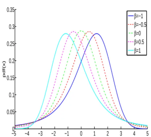
has an influence on the shape of the fSα(β,γ,δ). The curve has a large peak when α is near 0 and a Gaussian shape when
α = 2 (Figure 1(a)). The shape of the distribution skews to the left if β = 1, to the right if β = −1 (Figure 1(b))
while the distribution is symmetrical when β= 0. Finally, the scale parameter enlarges or compresses the shape of the
distribution (Figure 1(c)) and the location parameter leads to the translation of the mode of the fSα(β,γ,δ)(Figure 1(d)).
2.4. An overview ofα-stable estimators
The estimators of α-stable distributions are decomposed into three families: • the sample quantile methods [21, 22]
• the sample characteristic function methods [23, 24, 25, 26] • the Maximum Likelihood Estimation [27, 28, 29, 30].
Fama and Roll [21] developed a method based on quantiles. However, the algorithm proposed by Fama and Roll
suffers from a small asymptotic bias in α and γ and restrictions on α ∈]0.6, 2] and β = 0. McCulloch [22] extended
the quantile method to the asymmetric case (i.e. β= 0). The McCulloch estimator is valid for α ∈]0.6, 2].
Press [23, 24] proposed a method based on transformations of characteristic function. In [31], the author
com-pared the performances of several estimators. For example, the Press method is efficient for specific values.
Koutrou-velis [25] extended the Press method and proposed a regression method to estimate the parameters of α-stable distri-butions. He proposed a second version of his algorithm which is distinct that it is iterative [26]. In [32], the authors proved that the method proposed by Koutrouvelis is better than both the quantile method and the Press method because it gives consistent and asymptotically unbiased estimates.
The Maximum Likelihood Estimation (MLE) was first studied in the symmetric case [27, 28]. Dumouchel [29] developed an approximate maximum likelihood method. The MLE was also developed in the asymmetric case.
Nolan [30] extended the MLE in general case. The problem with the MLE is the calculation of the α-stable proba-bility density function because there is no closed-form expression. Moreover, the computational algorithm is time-consuming.
Consequently, we estimate a univariate α-stable distribution using the Koutrouvelis method [26]. 2.5. Multivariate stable distributions
It is possible to extend the α-stable distributions to the multivariate case. A random vector X ∈ R is stable if for
all a, b ∈ R+, there are c ∈ R+and D ∈ Rdsuch that:
aX1+ bX2= cX + D, (4)
where X1and X2are two independent and identically distributed random vectors which follow the same distribution
as X.
The characteristic function of an multivariate α-stable distribution, denoted X ∼ Sα,d(σ, δ), has the form:
φSα,d(σ,δ)(t)= exp − Z Sd |< t, s > |α(1 − jsgn(< t, s >) tan(πα 2 )σ(ds)+ j < δ, t > ! if α , 1, exp − Z Sd |< t, s > |(1 + jπ 2sgn(< t, s >) ln(< t, s >))σ(ds)+ j < δ, t > ! if α= 1, (5) with
• Sd= {x ∈ Rd|||x||= 1} the d-dimensional unit sphere.
• σ(.) a finite Borel measure on Sd.
• δ, t ∈ Rd.
The expression for the characteristic function involves an integration over the unit sphere Sd. The measure σ is called
the spectral measure and δ is called the location parameter. The problem with a multivariate α-stable distribution is that characteristic function forms a non-parametric set. To avoid this problem, it is possible to consider a discrete spectral measure [33] which has the form:
σ(.) =
K
X
i=1
γiδsi(.), (6)
with γicorresponding to weight and δsithe Dirac measure in si. For an α-stable distribution in R
2with K mass points,
the quantity si= {cos(θi), sin(θi)} with θi=2π(i−1)K .
There are two methods to estimate an α-stable random vector: • the PROJection method [34] (PROJ)
• the Empirical Characteristic Function method [35] (ECF)
These two algorithms have the same performances in terms of estimation and computation time.
At this point, it is important to underline that the features extracted from mono-beam echo-sounders have the properties of heavy-tails and skewness. Consequently, we decided to estimate the data with an α-stable model. These data are however imprecise and uncertain: the imprecision and uncertainty of data can be linked to poor quality estimation of these data. To take these constraints into consideration, we used an uncertain theory called the theory of belief functions. Consequently, the goal of the next section is to present the theory of belief functions.
3. The belief functions
The final objective of this paper is to classify synthetic and real data using the theory of belief functions. Data obtained from sensors are generally imprecise and uncertain as noises can disrupt their acquisition. It is possible to consider these constraints by using the theory of belief functions. We will first develop the theory of belief functions within a discrete framework before characterizing it in real numbers.
3.1. Discrete belief functions
This section outlines basic tools in relation to the theory of belief functions. 3.1.1. Definitions
Discrete belief functions were introduced by Dempster [8], and formalized by Shafer [9] where he considers a
discrete set of n exclusive events Cicalled the frame of discernment:
Θ = {C1, . . . , Cn}. (7)
Θ can be interpreted as all the assumptions to a problem. Belief functions are defined as 2Θonto [0,1]. The objective
of discrete belief functions is to attribute a weight of belief to each element A ∈ 2Θ. Belief functions must follow the
normalization:
X
A⊆Θ
mΘ(A)= 1, (8)
where mΘis called the basic belief assignment (bba).
A focal element is a subset of A where mΘ(A) > 0 and several functions in one-to-one correspondence are built from
bba: belΘ(A) = X B⊆A,B,∅ mΘ(B), (9) plΘ(A) = X A∩B,∅ mΘ(B), (10) qΘ(A) = X B⊂Θ,B⊇A mΘ(B). (11)
The credibility function of A called belΘ(A) is all the elements B ⊆ A which believe partially in A. This function
can be interpreted as a minimum of belief in A. On the contrary, a plausibility function plΘ(A) illustrates the maximum
belief in A while commonality function qΘ(A) represents the sum of bba allocated to the superset of A. This function
is very useful as shown below. 3.1.2. Combination rule
We consider M different experts who give mass mΘ
i(i = 1, . . . , M) on each element A ⊆ Θ. Alternatively, it is
possible to combine them using combination rules. There are several combination rules [36] in the literature which
differently address conflicts between sources. The most common rule is the conjunctive combination [37] where the
resultant mass of A is obtained by:
mΘ(A)= X B1∩...Bn=A,∅ M Y i=1 mΘi (Bi) , ∀A ∈ 2Θ. (12)
The mass of the empty set is given by:
mΘ(∅)= X B1∩...Bn=∅ M Y i=1 mΘi(Bi) , ∀A ∈ 2Θ. (13)
This rule allows us to stay in the open world. However, this is not practical as calculations are difficult. It is possible
to calculate resultant mass with communality functions where each mass mΘi(i= 1, . . . , M) must be converted into its
communality function to calculate the resultant communality function as follows:
qΘ(A)=
M
Y
i=1
qΘi (A). (14)
3.1.3. Pignistic probability
To make a decision onΘ, several operators exist such that maximum credibility or maximum plausibility with
pignistic probability being the most commonly used operator [38]. This name comes from pignus, a bet, in Latin.
This operator approaches the pair (bel,pl) by uniformly sharing a mass of focal elements on each singleton Ci. This
operator is defined by:
betP(Ci)=
X
A⊂Θ,Ci∈A
mΘ(A)
|A|(1 − mΘ(∅)), (15)
where |A| represents the cardinality of A.
We choose the decision Ciby evaluating max
1≤k≤nbetP(Ck).
3.2. Continuous belief functions
The basic description of continuous belief functions was accomplished by Shafer [9], then by Nguyen [39] and Strat [40]. Recently, Smets [41] extended the definition of belief functions to the set of reals R = R ∪ {−∞, +∞} and masses are only attributed to intervals of R.
3.2.1. Definitions
Let us consider I= {[x, y], (x, y], [x, y), (x, y); x, y ∈ R} as a set of closed, half-opened and opened intervals of R.
Focal elements are closed intervals of R. The quantity mI(x, y) are basic belief densities linked to a specific pdf. If
x> y, then mI(x, y)= 0. With these definitions, it is possible to define the same functions as in the discrete case. The
interval [a, b] being a set of R with a ≤ b, the previous functions can be defined as follows:
belR([a, b]) = Z x=b x=a Z y=b y=x mI(x, y)dydx, (16) plR([a, b]) = Z x=b x=−∞ Z y=+∞ y=max(a,x) mI(x, y)dydx, (17) qR([a, b]) = Z x=a x=−∞ Z y=+∞ y=b mI(x, y)dydx. (18) 3.2.2. Pignistic probability
The definition of pignistic probability for a < b is:
Bet f([a, b])= Z x=+∞ x=−∞ Z y=+∞ y=x |[a, b] ∩ [x, y]| |[x, y]| m I(x, y)dxdy. (19)
It is possible to calculate pignistic probabilities to have basic belief densities. However, many basic belief densities exist for the same pignistic probability. To resolve this issue, we can use the consonant basic belief density. A basic
belief density is said to be “consonant” when focal elements are nested. Focal elements Iucan be labeled as an index
usuch that Iu ⊆ Iu0 with u
0 > u. This definition is used to apply the least commitment principle, which consists in
choosing the least informative belief function when a belief function is not totally defined and is only known to belong to a family of functions. The least commitment principle relies on an order relation between belief functions in order to determine if a belief function is more or less committed than another. For example, it is possible to define on order based on the commonality function:
(∀A ⊆Θ, qΘ1(A) ≤ qΘ2(A)) ⇔ (mΘ1 ⊆qmΘ2). (20)
The mass function mΘ2 is less committed than mΘ1 according to the commonality function.
The function Bet f can be induced by a set of isopignistic belief functions Biso(Bet f ). Many papers [41, 42, 43] deal with the particular case of continuous belief functions with nested focal elements. For example, Smets [41]
proved that the least committed basic belief assignment mRfor the commonality ordering attributed to an interval
I= [x, y] with y > x related to a bell-shaped1pignistic probability function is determined by2:
mR([x, y])= θ(y)δ
d(x − ζ(y)), (21)
with x= ζ(y) satisfying Bet f (ζ(y)) = Bet f (y) and θ(y):
θ(y) = (ζ(y) − y)dBet f(y)
dy . (22)
The resultant basic belief assignment mRis consonant and belongs to the set Biso(Bet f ). However, it is difficult to
build belief functions in the particular case of multimodal pdfs because the frame of discernment has connected sets. In [44, 45], the authors propose a way to build belief functions with connected sets by using a credal measure and an index function.
3.3. Credal measure and index function
In [44], the authors propose a way to calculate belief functions from any probability density function. They use an index function f and a specific index space I to scan the set of focal elements F :
fI : I → F, (23)
y 7−→ fI(y). (24)
The authors introduce a positive measure µΩsuch thatRIdµΩ(y) ≤ 1 describes unconnected sets. The pair ( fI, µΩ)
defines a belief function. For all A ∈Ω, they define subsets which belong to the Borel set:
F⊆A = {y ∈ I| fI(y) ⊆ A}, (25)
F∩A = {y ∈ I| fI(y) ∩ A , ∅}, (26)
F⊇A = {y ∈ I| fI(y) ⊇ A}. (27)
From these definitions, they compute belief functions:
belΩ(A) = Z F⊆A dµΩ(y), (28) plΩ(A) = Z F∩A dµΩ(y), (29) qΩ(A) = Z F⊇A dµΩ(y). (30)
They continue their study by considering consonant belief functions. The set of focal elements F must be ordered
from the operator ⊆. They define an index function f from R+to F such that:
y ≥ x=⇒ f (y) ⊆ f (x). (31)
They generate consonant sets by using a continuous function g from Rdto I= [0, αmax[. The α-cuts are the set:
fcsI = {x ∈ R
d|g(x) ≥ α}. (32)
They finally define the index function:
fcsI : I= [0, αmax] → { fcsI(α)|α ∈ I}, (33)
α 7−→ fI
cs(α). (34)
1i.e.the pdf is unimodal with a mode µ, continuous and strictly monotonous increasing (decreasing) at left (right) of the mode. 2δ
The information available is the conditional pignistic density Bet f . However, many basic belief densities exist for the same pignistic probability Bet f . The least commitment principle allows the least informative basic belief density to
be chosen, where the focal elements are the α-cuts of Bet f such that3:
dµΩ(y)(α)= λ( fI
cs(α))dλ(α). (35)
4. Continuous belief functions andα-stable distribution
In this section, we model data distributions as a single α-stable distribution. We must however introduce the notion of plausibility function for an α-stable distribution. We first describe how to calculate the plausibility function
knowing the pdf in R before we extend to in Rd. We finally explain how we construct our belief classifier.
4.1. Link between pignistic probability function and plausibility function in R
The information available is the conditional pignistic density Bet f [Ci] with Ci ∈ θ. The function Bet f [Ci] is
supposed to be bell-shaped for all α-stable distributions (proved by Yamazato [46]).
The plausibility function from a mass mRis obtained by an integral of Equation (22) between [x,+∞[:
plR[C i](I)= Z +∞ x (ζ(t) − t)dBet f(t) dt dt. (36)
By assuming that Bet f is symmetrical, an integration by parts can simplify Equation (36) :
plR[C
i](I)= 2(x − µ)Bet f (x) + 2
Z +∞
x
Bet f(t)dt. (37)
Now let us consider a particular case where symmetrical Bet f is an α-stable distribution (the parameter β= 0). We
already know that Bet f (x)= fSα(β,γ,δ)(x). We can calculate
R+∞
x Bet f(t)dt by using the Chasles’ theorem:
Z +∞ −∞ fSα(β,γ,δ)(t)dt= Z x −∞ fSα(β,γ,δ)(t)dt+ Z +∞ x fSα(β,γ,δ)(t)dt. (38)
By definition, a pd f has the quantityR−∞+∞fSα(β,γ,δ)(t)dt = 1 and R
x
−∞fSα(β,γ,δ)(t)dt represents the definition of the
α-stable cumulative density function FSα(β,γ,δ).
Consequently, Equation (37) can be simplified:
plR[C
i](I)= 2(x − µ) fSα(β,γ,δ)(x)+ 2(1 − FSα(β,γ,δ)(x)). (39)
The plausibility function related to an interval I = [x, y] can also be seen as the area defined under the αcut-cut such
that αcut= Bet f (x). The notation pl[Ci](x) is equivalent to pl[Ci](I).
Now us let consider an asymmetric α-stable probability density function. We must proceed numerically to
cal-culate plausibility function at point x1 > µ, with µ the mode of the probability density function (Figure 2). The
plausibility function related to an interval I1 = [x1, y1] is defined by the area defined under the αcut-cut such that
αcut= Bet f (x1): plR[C i](I1)= Z x1 −∞ Bet f(t)dt+ (y1− x1)Bet f (x1)+ Z +∞ y1 Bet f(t)dt. (40)
By definition, a pd f has the quantityR+∞
y1 fSα(β,γ,δ)(t)dt = 1 − FSα(β,γ,δ)(y1) and
Rx1
−∞fSα(β,γ,δ)(t)dt = FSα(β,γ,δ)(x1). In
general, we know only one point y1. We estimate numerically x1such that fSα(β,γ,δ)(y1) = fSα(β,γ,δ)(x1). Finally, the
plausibility function related to the interval I1is:
plR[C
i](I1)= 1 + FSα(β,γ,δ)(x1) − F(y1)+ (y1− x1) f (x1). (41)
In practice, we base the classification on several features defined for different classes Θ = {C1, .., Cn}. For example,
the Haralick parameters “contrast” and “homogeneity” have different values for the classes rock, silt and sand. The
features are modeled by a probability density function because the features have continuous values. We can calculate a plausibility function related to its probability density functions by using the least commitment principle. Several plausibility functions associated to the same feature can be combined by using the generalized Bayes theorem [47, 48] to calculate mass functions allocated to A of an interval I:
mR[x](A)=Y Cj∈A plj(x) Y Cj∈Ac (1 − plj(x)). (42)
For several features, it is possible to combine the mass functions with combination rules.
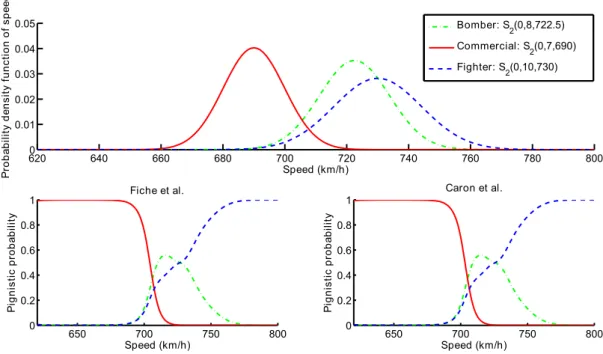
To validate our approach, we classify planes using kinematic data as in [42, 43] and compare the decision with the approach of Caron et al. [43]. We associate a Gaussian probability density function for each speed’s target (Figure 3):
• Commercial defined by the probability density function of speed S2(0, 8, 722.5).
• Bomber defined by the probability density function of speed S2(0, 7, 690).
• Fighter defined by the probability density function of speed S2(0, 10, 730).
We can observe that the decision is the same with the both approaches in the particular case of Gaussian probability density functions.
4.2. Link between pignistic probability function and plausibility function to Rd
It is possible to extend plausibility function in Rd. In [43], the authors calculate plausibility function in the
Gaussian pdf situation of mode δ and matrix of covarianceΣ. Mass function is built in such a way that isoprobability
surfaces Siwith 1 ≤ i ≤ n are focal elements. In R2, isoprobability points of a multivariate Gaussian pdf of mean
δ and covariance matrix Σ are ellipses. In dimension d, the authors defined focal elements as the nested sets HVα
enclosed by the isoprobability hyperconics HCα= {x ∈ Rd|(x − δ)tΣ−1(x − δ)}. They obtain bbd by applying the least
commitment principle: mRd(HV α)= α d+2 2−1 2d+22 Γ(d+2 2 ) exp (−1 2α) with α ≥ 0. (43)
Equation (43) defines a χ2distribution with d+ 2 degrees of freedom. The plausibility function at point x belonging
to a surface Si corresponds to the volume delimited by Si (we give an example in Figure 4 for an α-stable pdf).
Consequently, the plausibility function at point x is defined by:
plRd(x ∈ Rd)= Z α=+∞ α=(x−δ)tΣ−1(x−δ) αd+2 2 −1 2d+22 Γ(d+2 2 ) exp (−1 2α)dα. (44)
Equation (44) can be simplified by:
plRd(x ∈ Rd)= 1 − F
d+2((x − δ)(Σ)−1(x − δ)). (45)
The function Fd+2 is a cumulative density function of the χ2 distribution with d + 2 degrees of liberty (d is the
dimension of vector x).
The authors also calculate plausibility functions in the particular case of GMMs with their pdfs denoted by pGM M:
pGM M(x)=
k=n
X
k=1
wkN (x, δk, Σk), (46)
where N(x, δk, Σk) is the normal distribution of the k components with mean δkand matrix of covariance Σk and
plausibility function of the GMMs can be seen as a weighted sum of plausibility functions defined by each component of the mixture: plRd(x ∈ Rd)= 1 − k=n X k=1 wkFd+2((x − δk)(Σk)−1(x − δk)). (47)
We want to extend the calculation of plausibility function for any α-stable pdf. However, there is no closed-form expression for α-stable pdf. We use the approach developed by Dor´e et al. [44] to build belief functions.
4.3. Belief classifier
Let us consider a data set with N samples from d sensors. For example, each feature of a vector x ∈ Rd can
be seen as a piece of information from a sensor. The classification is divided into two steps. N × p (with p ∈]0, 1[) samples are first picked out randomly from the data set for the learning base, noted X, such that:
X= x1 1 . . . x N×p 1 .. . ... ... x1d . . . xN×pd
All columns of X belong to a class Ciwith 1 ≤ i ≤ n. Probability density functions (Gaussian or α-stable models)
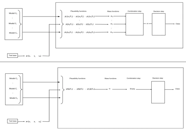
are estimated from samples belonging to classes. The rest of the samples is used for the test base (N × (1 − p) vectors). We use a validation test to determine if samples belong to an estimated model. If the test is not valid, we stop the classification, otherwise we continue the classification (Figure 5). The classification step diagram in one and
ddimensions is shown in Figure 6.
Plausibility functions knowing classes for x are calculated either from their probability density functions by using Equation (41) for an unsymmetric α-stable probability density function or by using Equation (45) for a Gaussian probability density function. We obtain d mass functions (one for each feature) at point x with the generalized Bayes theorem [47, 48] (Equation (42)). These d mass functions are combined by a combination rule to obtain a single mass function (section 3.1.2). Finally, the mass function is transformed into pignistic probability (Equation (19)) to make the decision.
It is also possible to work with a vector x of d dimensions. For an α-stable probability density function, plausibility functions are calculated for each feature by using the approach of Dor´e et al [44] (section 3.3). For a Gaussian probability density function, we use Equation (45) to calculate plausibilty functions. We calculate one mass function at point x by using the generalized Bayes theorem (Equation (42)). There is no combination step because we are calculating a single mass function. We use Equation (19) to transform the mass function into pignistic probabilities. The decision is chosen by using the maximum number of pignistic probabilities.
5. Application to pattern recognition
The aim is to build a belief classifier and to perform a classification of synthetic and real data by estimating features using a Gaussian and α-stable pdf. In [12], synthetic data are classified by modeling features using Gaus-sian and α-stable mixture models. By observing confidence intervals, the hypothesis of α-stable mixture models is significantly better than the hypothesis of Gaussian mixture models. However, when the number of Gaussian distribu-tions increases, classification accuracies are significantly the same. Images from a side-scan sonar are automatically classified by extracting Haralick features [49, 50]. However, classification accuracies are roughly the same.
In this section, we limit algorithms with a vector of features in dimension d ≤ 2. Indeed, the generalization of α-stable pdf in dimension d > 2 increases CPU time because there is no closed-form expression. Consequently, we distinguish two cases during the classification step:
• The one dimension case: each dimension is considered as a feature. • The two case: we considered a vector of two features.
We also use a statistical test called Kolmogorov-Smirnov test (K-S test) to evaluate the quality of each model. A
Kolmogorov-Smirnov test (K-S test) with a significance level of 5 % is also used to determine if two datasets differ
significantly. Let us assume two null hypotheses:
• H1: “Data follow a Gaussian distribution”.
• H2: “Data follow an α-stable distribution”.
The notation H1 and H2 are used for the rest of the paper. If the test rejects a null hypothesis Hi, we stop the
classification. Otherwise, if the test is valid, we then classify the samples belonging to the test base by using the belief classifier.
The results obtained with the belief functions are compared using a Bayesian approach. The prior probability p(Ci)
is first calculated corresponding to the proportion of each class in the learning set. For each class, the application of Bayes theorem gives posterior probabilities:
p(Ci/x) = p(x/Ci)p(Ci) n X u=1 p(x/Cu)p(Cu) . (48)
Finally, the decision is chosen by using the maximum nimber of posterior probabilities.
We first present a classification of synthetic data, belonging to Gaussian distributions, by modeling features using a Gaussian distribution and α-stable pdf. We then compare the α-stable and Gaussian model with synthetic data belonging to α-stable distributions. The same approach is finally applied to real data from a mono-beam echo-sounder. 5.1. Application to synthetic data generated by Gaussian distributions
In this subsection, we show that the α-stable and Gaussian model have the same behavior during the classification when synthetic data are generated by Gaussian distributions.
5.1.1. Presentation of the data
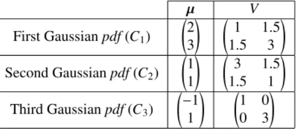
µ V First Gaussian pdf (C1) 2 3 ! 1 1.5 1.5 3 ! Second Gaussian pdf (C2) 1 1 ! 3 1.5 1.5 1 ! Third Gaussian pdf (C3) −1 1 ! 1 0 0 3 !
Table 1: Numerical values for the Gaussian pdf.
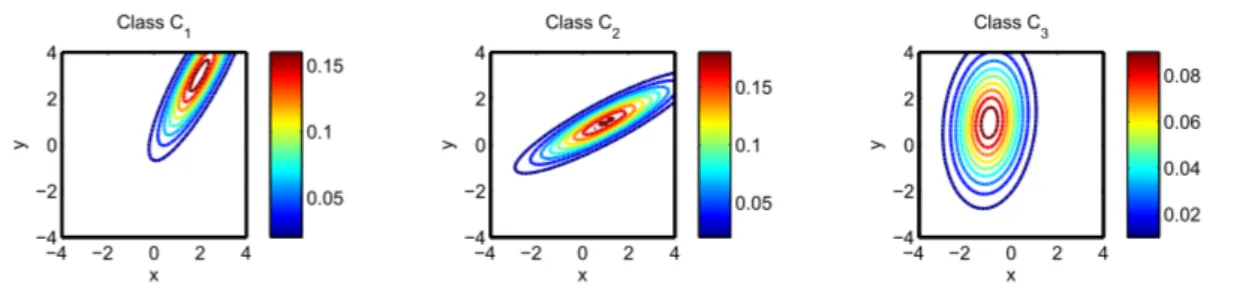
We simulated three Gaussian pdfs in R × R (c.f. Table 1). Each distribution holds 3000 samples. A mesh between [−4, 4] × [−4, 4] enables the level curves of pdf to be plotted (Figure 7).
5.1.2. Results
We generated data and split samples randomly into two sets: one third for the learning base and the rest for the test base. The learning base was used to estimate each mean and variance for the Gaussian distributions and each parameter α, β, γ and δ for the α-stable distributions [6, 25, 51]. We needed to make a mesh between [−4, 4] × [−4, 4]
to calculate plausibility functions in R2 with the α-stable model. Consequently, samples were chosen possessing
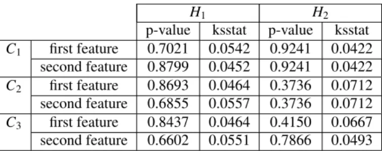
H1 H2
p-value ksstat p-value ksstat
C1 first feature 0.7021 0.0542 0.9241 0.0422 second feature 0.8799 0.0452 0.9241 0.0422 C2 first feature 0.8693 0.0464 0.3736 0.0712 second feature 0.6855 0.0557 0.3736 0.0712 C3 first feature 0.8437 0.0464 0.4150 0.0667 second feature 0.6602 0.0551 0.7866 0.0493
Table 2: Statistical values for a Kolmogorov-Smirnov test with a significance level of 5 % (p-value: the critical value to reject the null hypothesis, ksstat: the greatest discrepancy between the observed and expected cumulative frequencies).
The one dimension case.
For each class Ci, we consider each feature as a source of information. The estimated probability density functions
can be seen as pignistic probability functions. For each pignistic probability function, we associate a mass function which will subsequently be combined with other mass functions.
The K-S test is valid for the two null hypotheses H1 and H2 (Table 2). We can assert that samples are drawn
from the same distribution. The proposed method performs well in the particular case of synthetic data belonging to Gaussian distributions. However, the classification rates (Table 3) are very low because there is confusion between classes (Figure 8). The classification accuracy obtained with the Bayesian approach is significantly the same as the belief functions. Indeed, the Bayesian performs well provided that the probability density functions are well-estimated. The classification results depend on the prior probabilitiy estimation: if a prior probability of a class is underestimated, the confusion between classes increases.
We extended our study to a vector of two dimensions to try to improve the classification rate. The two dimension case.
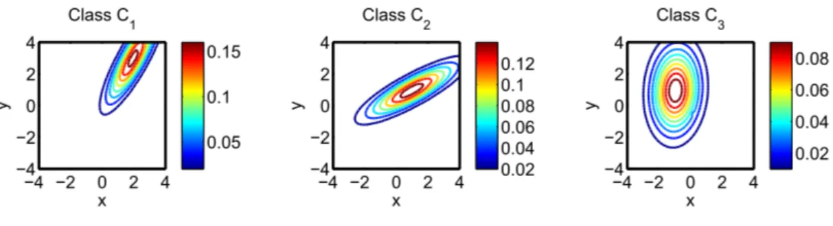
We generalized the study by considering a vector of two features. The learning base was used to estimate each mean and matrix of covariance for the Gaussian distributions (Figure 9) and each parameter α, σ, θ and δ for the α-stable distributions [35] (Figure 10).
As in one dimension, the two null hypotheses H1and H2were verified (Table 4). The classification results (Table 3)
are somewhat less than impressive because there is confusion between classes (between C1 and C2 cf. Figure 7).
Furthermore, the work in two dimensions enables better results to be obtained than the combination. The Bayesian approach gives significantly the same results as the theory of belief functions. Indeed, the estimations of model and the estimation of prior probabilities are well-estimated.
We extended our study by considering synthetic data generated by α-stable distributions.
Bayesian approach Belief approach
Classification accuracies (%) 95 % confidence intervals Classification accuracies (%) 95 % confidence intervals
H1 1 dimension 66.19 [65.13,67.25] 66.76 [65.71,67.81]
2 dimensions 76.14 [75.19,77.09] 75.35 [74.39,76.31]
H2 1 dimension 66.25 [65.19,67.31] 67.15 [66.10,68.20]
2 dimensions 76.31 [75.36,77.26] 74.50 [73.53,75,47]
Table 3: Classification accuracies and 95 % confidence intervals.
5.2. Application to synthetic data generated byα-stable distributions
In this subsection, we show the interest in modeling features in one and two dimensions with a single α-stable distribution.
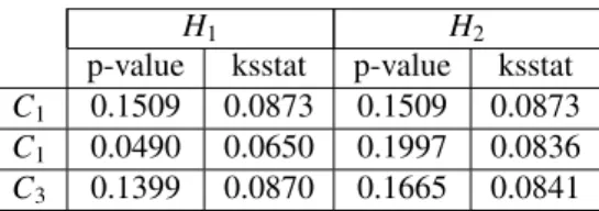
H1 H2
p-value ksstat p-value ksstat
C1 0.1509 0.0873 0.1509 0.0873
C1 0.0490 0.0650 0.1997 0.0836
C3 0.1399 0.0870 0.1665 0.0841
Table 4: Statistical values for a Kolmogorov-Smirnov test with a significance level of 5 % (p-value: the critical value to reject the null hypothesis, ksstat: the greatest discrepancy between the observed and expected cumulative frequencies).
α σ θ δ First α-stable pdf (C1) 1.5 1 1 ! 0 π 2 ! 0 0 ! Second α-stable pdf (C2) 1.5 1 1 ! 0 π 2 ! 2 1.4 ! Third α-stable pdf (C3) 1.5 1 1 ! 0 π 2 ! 1 0.5 !
Table 5: Numerical values for the α-stable pdf.
5.2.1. Presentation of the data
Three classes of artificial data sets were generated from 2D α-stable distributions [33] (c.f. Table 5 and [52] for the significance of σ and θ) with 3000 samples. A mesh between [−4, 4] × [−4, 4] enables the level curves of pdf to be plotted (Figure 11).
5.2.2. Results
The one dimension case.
We can assert that the estimation with the α-stable hypothesis is better than the Gaussian hypothesis (Figure 12).
There is a difference between the mode of the Gaussian model and the mode of α-stable model. Indeed, the mean,
calculated from samples, for the Gaussian model does not correspond to the mode when samples do not belong to a Gaussian law. Moreover, the values of pdfs are not the same compared to the real pdfs.
p-value ksstat C1 first feature 0.1758 0.0851 second feature 0.7614 0.0517 C2 first feature 0.8487 0.0458 second feature 0.4794 0.0630 C3 first feature 0.5505 0.0621 second feature 0.2753 0.0776
Table 6: Statistical values for a Kolmogorov-Smirnov test with a significance level of 5 % (p-value: the critical value to reject the null hypothesis, ksstat: the greatest discrepancy between the observed and expected cumulative frequencies).
The K-S test is not satisfied for the null hypothesis H1 for each class and each component. Consequently, we
stopped the classification step for the Gaussian model. However, the K-S test is valid for the null hypothesis H2
(Table 6). We can observe that the results obtained with the theory of belief functions are significantly the same as the results obtained using the Bayesian approach. This phenomenon can be explained by the fact that prior probabilities were well-estimated. Consequently, we changed voluntarily the values of prior probabilities. We fixed arbitrarily the
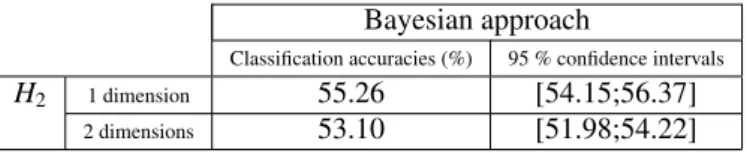
prior probabilities: p(C1) = 1/6, p(C2) = 2/3 and p(C3) = 1/6. The classification accuracy decreased to 53.10 %
(Table 7). Indeed, the learning base and the test base can sometimes be significantly different. For example, the prior probability of class sand can be greater than the prior probabilities of classes rock and silt, although it does not
represent the truth, and the classification rate of class sand can be favoured. This phenomenon introduces confusion between classes and the classification rate can decrease. Consequently, the learning step is an important step for the
Bayesian approach and can have a bad effect on the classification rate whereas the theory of belief functions is less
sensitive to the learning step.
Bayesian approach
Classification accuracies (%) 95 % confidence intervals
H2 1 dimension 55.26 [54.15;56.37]
2 dimensions 53.10 [51.98;54.22]
Table 7: Classification accuracies and 95 % confidence intervals with the prior probabilities p(C1)= 1/6, p(C2)= 2/3 and p(C3)= 1/6.
The two dimension case.
We considered a vector of two features. In Figure 13, we draw the iso-contour lines of data estimated with the Gaus-sian model and in Figure 14 the iso-contour lines of data estimated with the α-stable model
As in one dimension, the null hypothesis H1is rejected at significance level 5 %, but the null hypothesis H2is valid
(Table 8).
The classification results (Table 9) are somewhat less than impressive because there is confusion between classes. Furthermore, we obtain the same classification accuracies with the vector of two dimensions compared to the com-bination of two features. However, the classification decreases when the prior probabilities are not well-estimated (Table 7).
We also compared these results with a GMM. It is well-known that the GMM can accurately model an arbitrary
continuous distribution. This model estimation can be performed efficiently using the Expectation-Maximization
(EM) algorithm. We compared classification accuracies by increasing the number of components. We drew the classification accuracy (Figure 15) in relation to the number of components. Let us assume the null hypothesis:
• Gn: “Data follow a Gaussian mixture model with n components”.
The K-S test rejects the null hypothesis Gnfor a number of components n < 4. The representations of iso-contour
lines (Figure 16, Figure 17 and Figure 18) confirm the K-S test. Furthermore, the classification accuracies are lower than classification rates with a single α-stable pdf.
However, we can not increase indefinitely the number of components because a phenomenon of overfitting can appear (for example the representation of iso-contour by using a GMM with 5 components). Consequently, the number of 4 components seems to be a good compromise between the overfitting and good estimation. The classification accuracies are roughly the same between the single α-stable model and the GMM with 4 components.
p-value ksstat
C1 0.0683 0.1003
C1 0.3694 0.0688
C3 0.1154 0.0932
Table 8: Statistical values for a Kolmogorov-Smirnov test with a significance level of 5 % (p-value: the critical value to reject the null hypothesis, ksstat: the greatest discrepancy between the observed and expected cumulative frequencies).
5.3. Application to real data from a mono-beam echo-sounder 5.3.1. Presentation of data
We used a data set from a mono-beam echo-sounder given by the Service Hydrographique et Oc´eanique de la Marine (SHOM). Raw data represents an echo signal amplitude according to time. In [16], the authors classify seven types of sea floor by comparing the time envelope of echo signal amplitude with a set of theoretical references curves. In our application, raw data (Figure 19) were processed using the Quester Tangent Corporation (QTC) software [53] to
Bayesian approach Belief approach
Classification accuracies (%) 95 % confidence intervals Classification accuracies (%) 95 % confidence intervals
H2 1 dimension 66.56 [65.51;67.62] 66.49 [65.44;67.55]
2 dimensions 66.05 [64.99;67.11] 65.16 [64.08;66.22]
Table 9: Classification accuracies and 95 % confidence intervals.
obtain some features, which were normalized between [0,1]. These data had already been used for the navigation of an
Autonomous Underwater Vehicle (AUV) [54]. The frame of discernment isΘ = {silt, rock, sand}, with 4853 samples
from silt, 6017 from rock and 7338 from sand. The selection of features plays an important role in classification
because the classification accuracy can be different according to the features. In [55], the author gave an overview of
methods based on features to classify data and choose features which discriminate all classes. Some features calculated by the QTC software can be modeled by an α-stable pdf. There is a graphical test called converging variance test [56] which enables us to determine if samples belong to an α-stable distribution. This test calculates the estimation of variances by varying the number of samples. If the estimation of variance diverges, the samples can belong to an α-stable distribution. We give an example of this test for the feature called “third quantile calculated on echo signal amplitude” of the class rock (Figure 20). We chose the features called the “third quantile calculated on echo signal amplitude” and the “25th quantile calculated on cumulative energy”.
5.3.2. Results
We randomly select 5000 samples for the data set. Half the samples were used for the learning base and the rest for the test base. We first consider features in one dimension, i.e. two mass functions were calculated and combined to obtain a single mass function.
The one dimension case.
We can observe that the assumption of the α-stable model can easily accommodate the data compared to the Gaussian model (Figure 21).
The α-stable hypothesis is valid with the K-S test whereas the K-S test rejects the Gaussian hypothesis (Table 10). The approach using the theory of belief functions (classification accuracy of 82.68 %) give better results than the Bayesian approach (classification accuracy of 80.64 %) but not significantly. This phenomenon can be explained by the fact that the estimated models and prior probabilities are well-estimated.
The two dimensions case.
We extended the study by using a vector of two features. The level curves of empirical data (Figure 22) show there is confusion between the class silt and the class sand. The α-stable model (Figure 23) considers the confusion between classes compared to the Gaussian model (Figure 24).
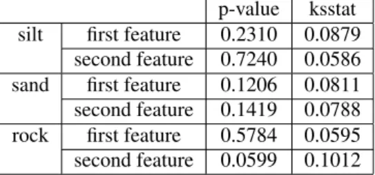
p-value ksstat
silt first feature 0.2310 0.0879
second feature 0.7240 0.0586
sand first feature 0.1206 0.0811
second feature 0.1419 0.0788
rock first feature 0.5784 0.0595
second feature 0.0599 0.1012
Table 10: Statistical values for a Kolmogorov-Smirnov test with a significance level of 5 % (p-value: the critical value to reject the null hypothesis, ksstat: the greatest discrepancy between the observed and expected cumulative frequencies.)
6. Conclusions
In this paper, we have shown the advantages in using the α-stable distributions to model data with heavy-tails. We
considered the imprecision and uncertainty of data for modeling pdf and the theory of belief functions offers a way
to model these constraints. We have examined the fundamental definitions of this theory and have shown a way to calculate plausibility functions when the knowledge of sensors is an α-stable pdf. We finally validated our model by making a comparison with the model examined by Caron et al. [43] where the pdf is a Gaussian.
Synthetic and real data were finally classified using the theory of belief functions. We estimated the learning base, calculated plausibility functions, combined plausibility functions and calculated maximum pignistic probability to obtain the classification accuracy. The K-S test shows that synthetic data can be modeled by an α-stable model. The proposed method performs well for synthetic data. The consideration of two features improves the classification rate compared to the combination of two features for the Gaussian data. This study was then extended to a real application by using features extracted from a mono-beam echo-sounder. The Gaussian model is limited when modeling features compared to the α-stable model because the α-stable model has more degrees of freedom. To sum up, the interest in using an α-stable model is that data, in both one or two dimensions, can be modeled. The problem with the α-stable model is the computation time. Indeed, we proceed numerically to calculate plausibility functions (discretization for
the bivariate α-stable pdf). Furthermore, it is difficult to generalize in dimension d > 2 without increasing CPU time.
We present preliminary results about classification problem by modeling features with α-stable probability density functions in dimension d ≤ 2. In future works, we plan to make experiments in the high-dimensional case with d ≥ 3. One solution in perspective to improve the computation time is to optimize the code in another language such that
C/C++. Another perspective to this work is the use of other features from sensors to improve the classification
accuracy, images from side-scan sonar.
Acknowledgements
The authors would like to thank the Service Hydrographique et Oc´eanique de la Marine (SHOM) for the data and G. Le Chenadec for his advice concerning the data.
References
[1] P. L´evy, Th´eorie des erreurs : La loi de Gauss et les lois exceptionnelles, Bulletin de la Soci´et´e Math´ematique de France. 52 (1924) 49-85. [2] A. Achim, P. Tsakalides, A. Bezerianos, SAR image denoising via Bayesian wavelet shrinkage based on heavy-tailed modeling, IEEE
Transactions on Geoscience and Remote Sensing. 41 (8) (2003) 1773-1784.
[3] A. Banerjee, P. Burlina, R. Chellappa, Adaptive target detection in foliage-penetrating SAR images using alpha-stable models, IEEE Trans-actions on Image Processing. 8 (12) (1999) 1823-1831.
[4] E.E. Kuruoglu, J. Zerubia, Skewed α-stable distributions for modelling textures, Pattern Recognition Letters. 24 (1-3) (2003) 339-348. [5] J.H. McCulloch, Financial applications of stable distributions, Handbook of statistics, Statistical Method in Finance. 14 (1996) 393-425. [6] E.F. Fama, The behavior of stock-market prices, Journal of business. 38 (1) (1965) 34-105.
[7] D.P. Williams, Bayesian Data Fusion of Multi-View Synthetic Aperture Sonar Imagery for Seabed Classification, IEEE Transactions on Image Processing. 18 (6) (2009) 1239-1254.
[8] A. Dempster, Upper and Lower probabilities induced by a multivalued mapping, Annals of Mathematical Statistics. 38 (2) (1967) 325-339. [9] G. Shafer, A mathematical theory of evidence, Princeton University Press, 1976.
[10] A. Fiche, A. Martin, Bayesian approach and continuous belief functions for classification, in: Proceedings of the Rencontre francophone sur la Logique Floue et ses Applications, Annecy, France, 5-6 November 2009.
[11] A. Dempster, N. Laird, D. Rubin, Maximum likelihood from incomplete data via the EM algorithm, Journal of the Royal Statistical Society B. 39 (1977) 1-38.
[12] A. Fiche, A. Martin, J.C. Cexus, A. Khenchaf, Influence de l’estimation des param`etres de texture pour la classification de donn´ees complexes, in: Proceedings of the Workshop Fouilles de donn´ees complexes, Brest, France, 25-28 January 2010.
[13] A. Fiche, A. Martin, J.C. Cexus, A. Khenchaf, Continuous belief functions and α-stable distributions, in: Proceedings of the 13th International Conference on Information Fusion, Edinburgh, United Kingdom, 26-29 July 2010.
[14] I. Quidu, J.P. Malkasse, G. Burel, P. Vilb´e. Mine classification based on raw sonar data: an approach combining Fourier descriptors, statistical models and genetic algorithms, in: Proceedings OCEANS2000 MTS/IEEE, Providence, Rhode Island, 2000, pp. 285-290.
[15] H. Laanaya, A. Martin,Multi-view fusion based on belief functions for seabed recognition, in: Proceedings of the 12th International Confer-ence on Information Fusion, Seattle, USA, 6-9 July 2009.
[16] E. Pouliquen, X. Lurton, Sea-bed identification using echo-sounder signals, in: Proceedings of the European Conference on Underwater Acoustics, Elsevier Applied Science, London and New York, 1992, pp. 535-539.
[18] M.S. Taqqu, G. Samorodnisky, Stable non-gaussian random processes, Chapman and Hall, 1994.
[19] V.M. Zolotarev, One-dimensional stable distributions, Translations of Mathematical Monographs Volume 65, American Mathematical Soci-ety, 1986.
[20] J.P. Nolan, Numerical calculation of stable densities and distribution functions, Communications in Statistics-Stochastic Models. 13 (4) (1997) 759-774.
[21] E.F. Fama, R. Roll, Parameter estimates for symmetric stable distributions, Journal of the American Statistical Association. 66 (334) (1971) 331-338.
[22] J.H. McCulloch, Simple consistent estimators of the parameters of stable laws, Journal of the American Statistical Association. 75 (372) (1980) 918-928.
[23] S.J. Press. Applied multivariate analysis, Holt, Rinehart and Winston New York, 1972.
[24] S.J. Press. Estimation in univariate and multivariate stable distributions, Journal of the American Statistical Association. 67 (340) (1972) 842-846.
[25] I.A. Koutrouvelis, Regression-type estimation of the parameters of stable laws, Journal of the American Statistical Association. 75 (372) (1980) 918-928.
[26] I.A. Koutrouvelis, An iterative procedure for the estimation of the parameters of stable laws, Communications in Statistics-Simulation and Computation. 10 (1) (1981) 17-28.
[27] B.W. Brorsen, S.R. Yang, Maximum likelihood estimates of symmetric stable distribution parameters, Communications in Statistics-Simulation and Computation. 19 (4) (1990) 1459-1464.
[28] J.H. McCulloch, Linear regression with stable disturbances, in: R. Adler, R. Feldman, M.S. Taqqu (Eds.), A practical guide to heavy tailed data, Birkh¨auser, Boston, 1998, pp. 359-376.
[29] W.H. Dumouchel, Stable distributions in statistical inference, Ph.D. dissertation, Department of statistics, Yale University, 1971.
[30] J.P. Nolan, Maximum likelihood estimation and diagnostics for stable distributions, in: O.E. Barndoff-Nielsen, T. Mikosh, S. Resnick (Eds.), L´evy processes: theory and applications, Birkh¨auser, Boston, 2001, pp. 379-400.
[31] R. Weron, Performance of the estimators of stable law parameters, Technical Report HSC/95/01, Hugo Steinhaus Center, Wroclaw University of Technology, 1995.
[32] V. Akgiray, C.G. Lamoureux, Estimation of stable-law parameters: A comparative study, Journal of Business & Economic Statistics. 7 (1) (1989) 85-93.
[33] R. Modarres, J.P. Nolan, A method for simulating stable random vectors, Computational Statistics. 9 (4) (1994) 11-20.
[34] J.H. McCulloch, Estimation of the bivariate stable spectral representation by the projection method, Computational Economics. 16 (1) (2000) 47-62.
[35] J.P. Nolan, A.K. Panorska, J.H. McCulloch, Estimation of stable spectral measures, Mathematical and Computer Modelling. 34 (9-11) (2001) 1113-1122.
[36] K. Sentz, S. Ferson, Combination of evidence in Dempster-Shafer theory, Technical Report, 2002.
[37] Ph. Smets, The combination of evidence in the transferable belief model, IEEE Transactions on Pattern Analysis and Machine Intelligence. 12 (5) (1990) 447-458.
[38] Ph. Smets, Constructing the pignistic probability function in a context of uncertainty, in: M. Henrion, R.D. Shachter, L.N. Kanal, J.F. Lemme (Eds.), Uncertainty in Artificial Intelligence 5, North Holland, Amsterdam, 1990, pp. 29-40.
[39] H.T. Nguyen. On random sets and belief functions, Journal of Mathematical Analysis and Applications. 65 (3), (1978) 531-542.
[40] T.M. Strat, Continuous belief functions for evidential reasoning, in: Proceedings of the National Conference on Artificial Intelligence, Austin, Texas, 1984, pp. 308-313.
[41] Ph. Smets, Belief functions on real numbers, International Journal of Approximate Reasoning. 40 (3) (2005) 181-223.
[42] B. Ristic, Ph. Smets, Target classification approach based on the belief function theory, IEEE Transactions on Aerospace and Electronic Systems. 42 (2) (2005) 574-583.
[43] F. Caron, B. Ristic, E. Duflos, P. Vanheeghe, Least Committed basic belief density induced by a multivariate Gaussian pdf, International Journal of Approximate Reasoning. 48 (2) (2008) 419-436.
[44] P.E. Dor´e, A. Martin, A. Khenchaf, Constructing of a consonant belief function induced by a multimodal probability density function, in: Proceedings of COGnitive systems with Interactive Sensors (COGIS09), Paris, France, 5-6 November 2009.
[45] J.M. Vannobel, Continuous belief functions: singletons plausibility function in conjunctive and disjunctive combination operations of conso-nant bbds, in: Proceedings of the Workshop on the Theory of Belief Function, Brest, France, 1-2 April 2010.
[46] M. Yamazato. Unimodality of infinitely divisible distribution functions of class L, The Annals of Probability. 6 (1978) 523-531.
[47] Ph. Smets, Belief functions: The disjunctive rule of combination and the generalized Bayesian theorem, International Journal of Approximate Reasoning. 9 (1) (1993) 1-35.
[48] F. Delmotte, Ph. Smets, Target identification based on the transferable belief model interpretation of Dempster–Shafer model, IEEE Transac-tions on Systems, Man and Cybernetics. 34 (4) (2004) 457-471.
[49] R.M. Haralick, K. Shanmugam, I.H. Dinstein, Textural features for image classification, IEEE Transactions on Systems, Man and Cybernetics. 3 (6) (1973) 610-621.
[50] R.M. Haralick, Statistical and structural approaches to texture, Proceedings of the IEEE. 67 (5) (1979) 786-804.
[51] J.H. McCulloch, Simple consistent estimators of stable distribution parameters, Communications in Statistics-Simulation and Computation. 15 (4) (1986) 1109-1136.
[52] J.P. Nolan, B. Rajput, Calculation of multidimensional stable densities, Communications in Statistics-Simulation and Computation. 24 (3) (1995) 551-566.
[53] D. Caughey, B. Prager, J. Klymak. Sea bottom classification from echo sounding data. Quester Tangent Corporation, Marine Technology Center, British Columbia, V8L 3S1, Canada, 1994.
[54] A. Martin, J.C. Cexus, G. Le Chenadec, E. Cant´ero, T. Landeau, Y. Dupas, R. Courtois, Autonomous Underwater Vehicle sensors fusion by the theory of belief functions for Rapid Environment Assessment, in: Proceedings of the 10th European Conference on Underwater Acoustics,
Istanbul, Turkey, 5-9 july 2010.
[55] I. Karoui, R. Fablet, J.M. Boucher, J.M. Augustin, Seabed segmentation using optimized statistics of sonar textures, IEEE Transactions on Geoscience and Remote Sensing. 47 (16) (2009) 1621-1631.
[56] C.W.J. Granger, D. Orr, ”Infinite Variance” and Research Strategy in Time Series Analysis, Journal of the American Statistical Association. 67 (1972) 275-285.
−50 −4 −3 −2 −1 0 1 2 3 4 5 0.1 0.2 0.3 0.4 0.5 0.6 0.7 x pdf(x) α=2 α=1.5 α=1 α=0.5
(a) Influence of parameter α with β= 0, γ = 1 and δ = 0.
−50 −4 −3 −2 −1 0 1 2 3 4 5 0.05 0.1 0.15 0.2 0.25 0.3 0.35 x pdf(x) β=−1 β=−0.5 β=0 β=0.5 β=1
(b) Influence of parameter β with α= 1.5, γ = 1 and δ = 0.
−50 −4 −3 −2 −1 0 1 2 3 4 5 0.1 0.2 0.3 0.4 0.5 0.6 0.7 0.8 x pdf(x) γ =1 3 γ =1 2 γ = 1 γ = 2 γ = 3
(c) Influence of parameter γ with α= 1.5, β = 0 and δ = 0.
−50 −4 −3 −2 −1 0 1 2 3 4 5 0.05 0.1 0.15 0.2 0.25 0.3 0.35 x pdf(x) δ=−2 δ=0 δ=2
(d) Influence of parameter δ with α= 1.5, β = 0 and γ = 1.
Figure 1: Different α-stable pdf.
pdf(μ)
y1 x1=ζ(b) μ αcut
pl([x1,y1])
620 640 660 680 700 720 740 760 780 800 0 0.01 0.02 0.03 0.04 0.05 Speed (km/h) Pr o b ab ili ty d en si ty f u n ct io n o f s p ee d Bomber: S2(0,8,722.5) Commercial: S2(0,7,690) Fighter: S2(0,10,730) 650 700 750 800 0 0.2 0.4 0.6 0.8 1 Speed (km/h) Pi g n is ti c p ro b ab ili ty Fiche et al. 650 700 750 800 0 0.2 0.4 0.6 0.8 1 Speed (km/h) Pi g n is ti c p ro b ab ili ty Caron et al.
Figure 3: Representation of probability density function of speed and the pignistic probabilities calculated from the Fiche et al. and Caron et al.[43] approaches. −2 −1.5 −1 −0.5 0 0.5 1 1.5 2 −2 −1.5 −1 −0.5 0 0.5 1 1.5 2 0.05 0.1 0.15 0.2 0.25 0.3 0.35 0.4 0.45 0.5
Data set
Learning base Test base
Estimation Validation test N samples N*p samples N*(1-p) samples Classification parameters of class Ci End If the test is not valid If the test is valid Class
Figure 5: Scheme of classification.
Plausibility functions ... ... ... ... ... ... ... ... Mass functions m1 mj md ... ...
Combination step Decision step
pld(xd/C1) pld(xd/Ci) pld(xd/Cn) plj(xj/C1) plj(xj/Ci) plj(xj/Cn) pl1(x1/C1) pl1(x1/Ci) pl1(x1/Cn) m ... ... m Empty pl(x/C1) pl(x/Ci) pl1(x/Cn)
Plausibility functions Mass functions Combination step Decision step
Class Test base x=[x1 xj xd] Class Test base x=[x1 xj xd] Model C1 Model Ci Model Cn .. . ... Model C1 Model Ci Model Cn .. . ...
x y Class C1 −4 −2 0 2 4 −4 −2 0 2 4 0.05 0.1 0.15 x y Class C2 −4 −2 0 2 4 −4 −2 0 2 4 0.05 0.1 0.15 x y Class C3 −4 −2 0 2 4 −4 −2 0 2 4 0.02 0.04 0.06 0.08
Figure 7: Iso-contour lines of generated Gaussian pdf.
−20 0 20 0 0.1 0.2 0.3 0.4 x pdf(x) C1 −20 0 20 0 0.05 0.1 0.15 0.2 0.25 x pdf(x) C2 −20 0 20 0 0.1 0.2 0.3 0.4 0.5 x pdf(x) C3 −20 0 20 0 0.05 0.1 0.15 0.2 0.25 x pdf(x) C 1 −20 0 20 0 0.1 0.2 0.3 0.4 x pdf(x) C 2 −20 0 20 0 0.1 0.2 0.3 x pdf(x) C 3
bar chart of data Gaussian pdf α−stable pdf
Figure 8: Empirical pdf and its estimations (The first row corresponds to the first feature and the second row corresponds to the second feature).
x y Class C1 −4 −2 0 2 4 −4 −2 0 2 4 0.05 0.1 0.15 x y Class C2 −4 −2 0 2 4 −4 −2 0 2 4 0.05 0.1 0.15 x y Class C3 −4 −2 0 2 4 −4 −2 0 2 4 0.02 0.04 0.06 0.08
x y Class C1 −4 −2 0 2 4 −4 −2 0 2 4 0.05 0.1 0.15 x y Class C2 −4 −2 0 2 4 −4 −2 0 2 4 0.02 0.04 0.06 0.08 0.1 0.12 x y Class C3 −4 −2 0 2 4 −4 −2 0 2 4 0.02 0.04 0.06 0.08
Figure 10: Iso-contour lines of data estimated with an α-stable model.
x y Class C1 −4 −2 0 2 4 −4 −2 0 2 4 0.02 0.04 0.06 x y Class C2 −4 −2 0 2 4 −4 −2 0 2 4 0.02 0.04 0.06 x y Class C3 −4 −2 0 2 4 −4 −2 0 2 4 0.02 0.04 0.06
Figure 11: Iso-contour lines of generated α-stable pdf.
−20 0 20 0 0.05 0.1 0.15 0.2 0.25 0.3 0.35 x pdf(x) C 1 −20 0 20 0 0.05 0.1 0.15 0.2 0.25 x pdf(x) C 2 −20 0 20 0 0.05 0.1 0.15 0.2 0.25 0.3 0.35 x pdf(x) C 3 −20 0 20 0 0.05 0.1 0.15 0.2 0.25 0.3 0.35 x pdf(x) C1
normalized bar chart of data normalized α−stable pdf normalized Gaussian pdf
−20 0 20 0 0.05 0.1 0.15 0.2 0.25 0.3 0.35 x pdf(x) C2 −20 0 20 0 0.05 0.1 0.15 0.2 0.25 x pdf(x) C3
x y Class C1 −4 −2 0 2 4 −4 −2 0 2 4 4 6 8 10 x 10−3 x y Class C2 −4 −2 0 2 4 −4 −2 0 2 4 0.005 0.01 0.015 0.02 x y Class C3 −4 −2 0 2 4 −4 −2 0 2 4 2 4 6 8 x 10⁻³
Figure 13: Iso-contour lines of data estimated with a Gaussian model.
x y Class C1 −4 −2 0 2 4 −4 −2 0 2 4 0.02 0.04 0.06 0.08 x y Class C2 −4 −2 0 2 4 −4 −2 0 2 4 0.01 0.02 0.03 0.04 0.05 x y Class C3 −4 −2 0 2 4 −4 −2 0 2 4 0.02 0.04 0.06
Figure 14: Iso-contour lines of data estimated with an α-stable model.
1 1.5 2 2.5 3 3.5 4 4.5 5 55 60 65 70 Number of components Classification rate α−stable model Gaussian model
Confidence interval for the α−stable model
Confidence intervals for the Gaussian model
x y −4−2 0 2 4 −4 −20 2 4 0.01 0.02 0.03 x y −4−2 0 2 4 −4 −20 2 4 0.02 0.04 0.06 x y −4−2 0 2 4 −4 −20 2 4 0.02 0.04 0.06 0.08 x y −4−2 0 2 4 −4 −20 2 4 0.02 0.04 0.06 0.08
Figure 16: Representation of iso-contour by modeling data with a mixture of Gaussian for the class C1(from left to right: 2, 3, 4 and 5 components).
x y −4−2 0 2 4 −4 −20 2 4 0.01 0.02 0.03 x y −4−2 0 2 4 −4 −20 2 4 0.02 0.04 x y −4−2 0 2 4 −4 −20 2 4 0.02 0.04 x y −4−2 0 2 4 −4 −20 2 4 0.02 0.04 0.06
Figure 17: Representation of iso-contour by modeling data with a mixture of Gaussian for the class C2(from left to right: 2, 3, 4 and 5 components).
x y −4−2 0 2 4 −4 −2 0 2 4 0.01 0.02 0.03 x y −4−2 0 2 4 −4 −2 0 2 4 0.02 0.04 x y −4−2 0 2 4 −4 −2 0 2 4 0.02 0.04 0.06 x y −4−2 0 2 4 −4 −2 0 2 4 0.02 0.04 0.06
0 50 100 150 200 250 300 350 400 450 0 0.01 0.02 0.03 0.04 0.05 time dB
Figure 19: Example of echo signal amplitude from silt in low frequency.
0 100 200 300 400 500 600 700 800 900 1000 0 0.01 0.02 0.03 0.04 0.05 0.06 Number of samples Sample variances
0 0.5 1 0 1 2 3 4 5 x pdf(x) silt 0 0.5 1 0 2 4 6 x pdf(x) sand 0 0.1 0.2 0.3 0.4 5 10 15 20 25 x pdf(x) rock 0.9 0.95 1 5 10 15 20 25 30 x pdf(x) silt 0.85 0.9 0.95 1 20 40 60 80 x pdf(x) sand 0.85 0.9 0.95 1 0 10 20 30 40 x pdf(x) rock
bar chart of data Gaussian pdf α stable pdf
Figure 21: Empirical pdf and its estimations (The first row corresponds to the feature called “third quantile calculated on echo signal amplitude” and the second row corresponds to the feature called “25th quantile calculated on cumulative energy”).
0
0.2 0.4 0.6 0.8
0
0.2
0.4
0.6
0.8
x
y
0
0.2 0.4 0.6 0.8
0
0.2
0.4
0.6
0.8
x
y
0
0.2 0.4 0.6 0.8
0
0.2
0.4
0.6
0.8
x
y
Figure 22: Level curves of three empirical α-stable distributions with 10000 samples (The first column refers to the class rock, the second column refers to the class sand and the third column refers to the class silt).
x
y
0
0.5
1
0
0.5
1
x
y
0
0.5
1
0
0.5
1
x
y
0
0.5
1
0
0.5
1
Figure 23: Level curves with an α-stable model estimation (The first column refers to the class rock, the second column refers to the class sand and the third column refers to the class silt).
0
0.5
1
0
0.5
1
x
y
0
0.5
1
0
0.5
1
x
y
0
0.5
1
0
0.5
1
x
y
Figure 24: Level curves with a Gaussian model estimation (The first column refers to the class rock, the second column refers to the class sand and the third column refers to the class silt).