3D Measurement and Characterization of Ultra-precision Aspheric Surfaces

Science Arts & Métiers (SAM)

is an open access repository that collects the work of Arts et Métiers Institute of

Technology researchers and makes it freely available over the web where possible.

This is an author-deposited version published in: https://sam.ensam.eu

Handle ID: .http://hdl.handle.net/10985/8653

To cite this version :

Nadim EL HAYEK, Hichem NOUIRA, Nabil ANWER, Olivier GIBARU, Mohamed DAMAK, Pierre BOURDET - 3D Measurement and Characterization of Ultra-precision Aspheric Surfaces - 3D Measurement and Characterization of Ultra-precision Aspheric Surfaces p.000-000 - 2014

Any correspondence concerning this service should be sent to the repository Administrator : archiveouverte@ensam.eu

Procedia CIRP 00 (2014) 000–000

13th CIRP Conference on Computer Aided Tolerancing

3D Measurement and Characterization of Ultra-precision Aspheric

Surfaces

N. El-Hayek

, N. Anwer

, H. Nouira

, O. Gibaru

, M. Damak

, P. Bourdet

a_{Arts et Métiers ParisTech, Laboratory of information sciences and systems (LSIS), 8 Boulevard Louis XIV, 59046 Lille, France}

b_{Laboratoire Commun de Métrologie (LNE-CNAM), Laboratoire National de métrologie et d'Essais (LNE), 1 Rue Gaston Boissier, 75015 Paris,}

France

c_{ENS de Cachan, The University Research Laboratory in Automated Production, 61 avenue du Président Wilson, 94235 Cachan, France}

d_{GEOMNIA, 165 Avenue de Bretagne, EuraTechnologies 59000 Lille, France}

Abstract

Aspheric surfaces have become widely used in various fields ranging from imaging systems to energy and biomedical applications. Although many researches have been conducted to address their manufacturing and measurement, there are still challenges in form characterization of aspheric surfaces considering a large number of data points. This paper presents a comparative study of 3D measurement and form characterization of an aspheric lens using tactile and optical single scanning probing systems. The design of the LNE high precision profilometer, traceable to standard references is presented. The measured surfaces are obtained from the aforementioned system. They are characterized with large number of data points for which a suitable process chain is deployed. The form characterization of the aspheric surfaces is based on surface fitting techniques by comparing the measured surface with the design surface. A comparative study of registration methods and non-linear Orthogonal Least-Squares fitting Methods is presented. Experimental results are analyzed and discussed to illustrate the effectiveness of the proposed approaches.

© 2014 Published by Elsevier Ltd. Selection and/or peer-review under responsibility of CIRP CAT 2014.

Keywords: Aspheric surface; form characterization; high precision metrology; non linear least-squares method; computational metrology.

1. Introductiona

Aspheric surfaces have become widely used in various applications such as optics, photonics and biomedicine. The manufacturing and measurement of such elements is still a common challenge in industry as the form characterization of aspheric surfaces is not yet normalized. This process becomes even harder when considering a large number of measurement points.

This paper presents a comparison of two measurement techniques and of three different fitting algorithms for the form characterization of aspheric surfaces. Optical and tactile single scanning probe

* Corresponding author. Tel.: +33-(0)147402413; fax: +33-(0)14740220. E-mail

address: anwer@lurpa.ens-cachan.fr

systems are commonly used in dimensional metrology applications. However, in order to reach a nanometric level of accuracy in the masurement of aspheric lenses, ultra-high precision machines should be employed. Therefore, the design of the LNE's high precision profilometer, traceable to the SI meter definition is presented. Its architecture complies with the Abbe principle and its metrology loop is optimized. The performance and capability of the machine in the scope of aspheric lenses metrology are discussed.

The measured surfaces (MS) are obtained from the aforementioned system. They are characterized by a large number of data points (> 100,000 points) which will be processed following a suitable procedure. This paper emphasizes the importance of building a combinatorial structure through a meshing phase. The mesh, as a linear approximation of the underlying surface, gives an insight of its topology and geometry.

"N. El-Hayek et al" / Procedia CIRP 00 (2014) 000–000 Moreover, it conveys sampling information and spatial

distribution of the measured surface points.

The Design Surface (DS) of the aspheric lens can be described using different models. A conic-polynomial model which serves as a basis for aspheric lens specification, a discretized form of the polynomial into a set of reference points to create a nominal CAD form, and a mapping of that polynomial into a linear combination of orthogonal basis functions.

The form characterization of aspheric lenses is based on Orthogonal Least-Squares fitting techniques by comparing the measured surface with the design surface. A comparative study of an Iterative Closest Point (ICP) method and non-linear Orthogonal Least-Squares Optimization Methods is presented here.

Three fitting algorithms are compared based on their capacities to converge quickly with an acceptable accuracy, to manage a large volume of data and to be robust and numerically stable.

Experimental results are presented and discussed to illustrate the effectiveness of the proposed approaches.

2. LNE high precision profilometer

Measuring aspheric surfaces to an accuracy of few tens of nanometres remains an important challenge in manufacturing and metrology of freeform optics [1]. To achieve the best possible accuracies, specific ultra-high precision machines have been developed by the National Metrology Institutes (NMIs) that ensure the traceability chain. In this regard, a three-year project has been launched by the European Metrology Research Program (EMRP) [2] and encompasses a multitude of European National Metrology Institutes (LNE, PTB, VSL, METAS, SMD and CMI), industry and academia aiming at improving apparatus and methods for high-precision measurement of aspheric and freeform optics and characterizing their form. The apparatus are generally related to small-volume coordinate measuring machines that feature measuring ranges of hundreds of milimetres. These machines respect the Abbe principle, apply the dissociated metrological structure and incorporate high-precision mechanical guiding elements.

2.1. Description of the LNE high precision profilometer

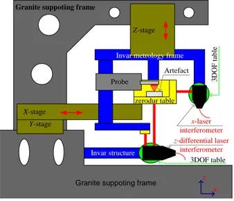
LNE's high precision profilometer is a measurement machine (Fig. 1) capable of performing independent motions in all x, y and z directions using three independent high-precision mechanical guiding systems equipped with encoders. While x and y motions are controlled by sub-nanometer resolution laser interferometers, the z motion is controlled by a differential laser interferometer that allows to shorten the metrology loop and maintain a sub nanometric accuracy.

Invar structure

Granite suppoting frame

Y-stage X-stage

Z-stage

x z Invar metrology frame

x-laser interferometer z-differential laser

interferometer

Granite suppoting frame

3D O F table 3DOF table Artefact Probe zerodur table

Fig. 1 Architecture of the LNE' high precision profilometer.

The working range in the xy-plane is 50×50 mm². The probe and its supporting structure are mounted on the vertical guiding system in the z-direction along which the measurement is done. The working range of the mechanical guiding system in z-direction is about 100 mm.The supporting frame is made of massive granite and carries the guiding elements. The metrology frame is made of Invar for minimal sensitivity to environmental influence.

The metrology loop incorporates three Renishaw laser interferometers and is equipped either with a chromatic confocal probe or a tactile probe to achieve nanometric resolution. The machine allows the in-situ calibration of the probes by means of a differential laser interferometer considered as a reference.

2.2. Evaluation of the LNE high precision profilometer

The uncertainty budget is established for the measurement of KNT4080-30 V-groove standards taking into consideration different and various error sources with the addition of the measuring probe's errors. The obtained results validate the cabability of the profilometer to perform measurement at the nanometer level of accuracy. Optical and tactile scanning of aspheric surfaces

The tactile and optical measurements of the asphere take place in the LNE's cleanroom in which environmental conditions are optimal. Temperature is controlled to 20±0.3 °C and humidity to 50±5 %RH.

The asphere is posed on the Zerodur table (Fig. 1) and is measured by a tactile single point scanning probe which has been previously calibrated in-situ. On this machine, it is not possible to exactly align the asphere's axis with the z axis of the measurement, however, an approximation of the apex position can be done by estimating the cusp of the surface. For this matter, the

surface is scanned once in the x- direction and once in the y- direction and a peak is computed. This peak represents an approximation of the cusp around which a symmetrical measurement is performed in x and y directions.

A large number of data points (>> 100,000 points) are recorded in the form of XY-grids (ranging from 5×5 mm² to 6×6 mm²). The optical probe's total measurement time is about half of the tactile probe's total measurement time since no contact needs to be established for the optical measurement.

2.3. Data structuring

The measured data are reported in Cartesian coordinates and a surface reconstruction algorithm is applied. A mesh is built and defines a structure on the points. It is a linear interpolation of the initially unstructured point set which becomes organized and structured. The mesh is a linear approximation of the underlying surface, which gives an insight of its topology and geometry. Discrete differential geometry parameters can be calculated and used for further processing such as filtration, partition and fitting.

3. Form characterization of aspheric surfaces

3.1. Mathematical representation of aspheric surfaces

The traditional way to represent aspheric surfaces is the axially symmetric quadric and power series parametric description as described in ISO 10110-Part 12 (Eq. 1)





,

1

1

1

cr

z

r

c r











 



where r is the radial coordinate, z is the sag (sagittal representation), c is the curvature at the apex, and  is the conic constant. The 2jr2j terms are the higher order aspheric terms that represent the additive departure from the quadric.

Other mathematical formulations have been developed [3]. Among them orthogonal basis polynomials such as Q-polynomials and Zernike polynomials in an attempt to improve the classic power series and representing the useful surface shape with a small number of parameters. This makes each term unique and meaningful.

3.2. Aspheric surface fitting

The form evaluation of aspheres can be done by performing the fitting or association of the aspheric

model to the measured data according to a criterion such as least-squares or minimum zone. The residuals of the fitting or the deviations to the associated reference model are then evaluated. The Peak-to-Valley (PV) and the Root Mean Square (RMS) are the most widely adopted parameters for the assessment of form deviations of aspheric surfaces.

Many fitting techniques are reported in the literature, but only few discuss the fitting of aspheres. Chen et al [4] propose an aspheric lens characterization by means of a 2D profile fitting. The dataset used is a profile measured using a stylus and the reference model is the corresponding asphere profile. The fitting is done using the Levenberg-Marquardt algorithm [5] for its quick convergence and precision. Similar works have been published and also deal with aspheric profile identification [6] and conic sections fitting [7]. Sun et al [8] perform fitting of aspheric curves and surfaces on simulated data with vertical distance minimization using a Gauss-Newton algorithm. In fact, they assume that the model and the data are both defined in the same reference frame. Other works involve approximating aspheres with NURBS models in order to generate CAD models for manufacturing purposes [9]. The problem of fitting the data to the aspheric surface model is posed as a nonlinear least-squares problem which is defined as follows (Eq. 2). 2 1

min

,

p

q



R

 

T

where  is the set of shape, position and orientation variables, R, T are transformation parameters, pi is a data point, and qi is the orthogonal projection of the data point pi onto the reference model (footpoint). In this paper, position and orientation parameters as well as shape parameters are estimated . The process described here goes by optimizing for five transformation parameters, the symmetry about z axis is being redundant here. The objective function to minimize is then given by the Eq. 3

2 , , , , , , , 1

min

,

p

q



R

 

T

Two general approaches to solving this problem can be considered. In the sequential approach, algorithms are implemented in sequential computation of footpoints and transformation parameters. Unlike sequential approaches, the simultaneous approach can perform optimization of transformation parameters and footpoints simultaneously.

There exists vast literature about non-linear least squares fitting algorithms. Gauss-Newton type [10] and

"N. El-Hayek et al" / Procedia CIRP 00 (2014) 000–000 Levenberg-Marquardt (LM) type [11] have been

recommended by NMIs. In this paper, we restrain the comparison to the sequential fitting implementation.

3.3. Orthogonal non-linear least squares fitting algorithms

The Newton-Raphson method [12] is usually used in optimization problems that are not highly non-linear even though the Hessian matrix can be approximated and second derivative calculations can be avoided. It will therefore be used in this paper for the computation of footpoints. The goodness of the approximation depends on the stop criterion and on the quality of the initial guess (relative position of the point data and the model should be close to the optimal solution) [12, 13].

For this problem, the vertical projection point is taken as an initial guess. Then, the Newton-Raphson method iterates until the orthogonal projection point is accurately approximated.

Levenberg-Marquardt [5, 14] is a well-known optimization algorithm that is based on an interpolation between a Gauss-Newton approach and the gradient descent. It has been approved by the National Institute of Standards and Technology (NIST) for metrology applications that require fitting simple curves and surfaces in 3D [11]. Generally, this algorithm converges reasonably quickly and accurately for a wide range of initial guesses that are relatively close to the optimal solution [4]. The fitting of parametric curves and surfaces using the LM algorithm also requires the calculation of a large Jacobian matrix and the storage of a considerable system of linear equations, as described by Speer et al [15].

For a very large number of variables or unconstrained non-linear problems, iterative quasi-Newton methods such as the Broyden-Fletcher-Goldfarb-Shanno (BFGS) method can be more convenient [16]. Like any minimization algorithm, BFGS preferably requires a twice differentiable objective function whose gradient must be zero at optimality. The method computes the Hessian of the function, therefore, a sequence of matrices is constructed through the iterations.

This sequence occupies a very large memory space which eventually comes to saturation when all the matrices are stored [17, 18]. Subsequently, Nocedal describes an improved method called L-BFGS which keeps updating the Hessian matrix using a limited amount of storage [17]. At every iteration, the Hessian is approximated using information from the last m iterations with each time, the new approximation replacing the oldest one in the queue. L-BFGS is an enhanced BFGS optimization algorithm for reducing memory usage when storage is critical and is suitable for applications involving large volumes of data and variables. Furthermore, Zheng et al [19] propose a

L-BFGS algorithm to perform B-Spline curve fitting and show that, unlike traditional methods, L-BFGS can perform optimization of control points and footpoints simultaneously.

3.4. Computational Geometry approaches

Computational geometry deals with the structure and complexity of discrete geometric objects as well as with the design of efficient computer algorithms for their manipulation. Registration and reconstruction are among the two most important research themes in computational geometry and can provide new research avenues to freeform surface fitting and Geometrical Product Specifications [20].

In previous work, a comparison of surface reconstruction algorithms for aspheric sufaces is presented. Delaunay and Voronoi-based meshing techniques are evaluated. The common approach for surface reconstruction is to build a 3D Delaunay triangulation and extract triangular facets that are a linear approximation of the underlying surface. The quality of the mesh sought is based on well-defined criteria. The reconstructed surface should topologically and geometrically be equivalent to the underlying surface of the points set. This lead to the choice of Cocone algorithm which fits at best our applications with the necessity of having an ε-sampled point set [21]. Another approach exploits that aspheric surface is a set of points that can be projected onto a plane following a bijective mapping without any superposition of points from different sides of the surface. The bijection property offers the advantage of tracing back the points to their original position without modifying either the geometry or the topology of the underlying surface. Since topology is preserved on the map, neighbourhood is conserved and points can thus be meshed in a 2D-like fashion. The data structure is built in 2D and then mapped back to 3D.

As a new alternative to the parametric description, a mesh-based representation of the aspheric surface is a refrence model when the problem needs to be expressed in discrete form.

The ICP (Iterative Closest Point) algorithm and its variants are the most popular methods for data registration [22, 23]. The ICP finds a spatial transformation to align two point-sets, making it a fast algorithm with negligible storage. It can be used for fitting applications when one of the point-sets is a theoretical point model or mesh model. ICP is based on two main operations, point identification and point matching and this operation is usually computationally expensive. An iterative loop identifies pairs of points and matches them across both entities.The matching phase results in a transformation matrix that brings one point-set to the other with residual error. If this error is

larger than the threshold value, point identification and matching restarts until the two point-sets are closely aligned. In order to have fine precision on the results, it is preferable that the size of both sets be equal.

For the mesh model case, the closest point is the footpoint of a data point on the closest triangle in the mesh. A mesh model offers the advantage of obtaining a more accurate distance calculation than a point model does. In general, dpm (point-to-mesh distance) is smaller

than dpp (point-to-point distance) and there are three

configurations for a point-to-mesh distance (point-vertex, point-edge, and point face). So in this case, the distance is calculated on a point-to-mesh distance following the mentioned three configurations.

4. Results and analysis

The comparison of the fitting algorithms is founded on two elements. Firstly, the effect of fitting data with orthogonal distance minimization is studied. Secondly, the effect of data size on the algorithms’ complexity is analyzed and is based on two criteria, the units of memory used and the computational time expressed as Central Processing Unit time (CPU time). In order to vary the number of points in a dataset, no specific filtration technique is applied, but simply, points are sampled at different chosen rates.

The machine used for the tests is an Intel core i7/x64 platform with 8 Gb of RAM and a 2.0 GHz processor.

4.1. Simulated datasets

The aspheric model is simulated based on Eq. 1 as shown in Fig. 2 by generating symmetrically distributed points around the asphere's axis. The design parameters of the asphere have the following values (c=10-20, κ=-1, α2=0.02227, α4=7.29×10-6, α6=4.52×10-9, α8=-1.061×10 -11_{, α}

10=9.887×10-15).

Then, simulations are performed in order to study the effect of data subject to errors both from measured object (form deviations) and measurement (Gauss noise) [24]. Measurement errors simulation involves generating Gaussian noise with controlled mean and standard deviation. This value is coherent with noise that can manifest on the measurement sensors. A MATLAB random function is used to generate this noise which is added to the theoretical data in the orthogonal direction at each data point. Fractional Brownian Motion is also superimposed on the theoretical data in order to simulate form deviations [25]. The H parameter (Hurst index) is taken to be 0.9 and the span equal to the number of points in the simulated dataset [26].

Fig. 2 Simulated asphere model without noise

The three fitting methods (LM, L-BFGS, and ICP) are used to fit and analyze the data and the results are compared. The output transformation parameters of each algorithm as well as the model parameters that are computed after each fit are also compared. The RMS and PV values are also reported in table 1. The RMS and PV of the simulated dataset are calculated upon generation and theoretically amount to 54.95 and 265.292 nm, respectively. From the results recorded in table 1, all three algorithms are equivalent with respect to the fitting parameters they output. The transformation parameters are almost identical across L-BFGS, LM and ICP. Since ICP is only an algorithm for fitting two datasets geometrically, the model parameters can't be estimated and the comparison in this matter restrains to L-BFGS and LM. The values of RMS and PV output by all three algorithms are very similar and are close to those of the simulated set. The fitted residual errors are slightly smaller than the theoretical values because there is a better position for the aspherical surface with respect to the generated Brownian motion errors.

This part validates the algorithms used for the purpose of fitting aspheric data. Their accuracy is acceptable and is equivalent across all of L-BFGS, LM and ICP. For a theoretical dataset simulated without any added noise, fitting returns parameters that are identical to the design parameters; whereas in the case of added noise, these parameters present a slight variation (especially α10).

"N. El-Hayek et al" / Procedia CIRP 00 (2014) 000–000

Table1. Fitting using Least-Squares orthogonal distance minimization for the combined systematic and random errors (N: Number of points; tp: transformation parameters; mp: model parameters).

N = 500,000 L-BFGS LM ICP tp Rx (°) Ry (°) tx (mm) ty (mm) tz (mm) -0.0086725 1.853623E-4 7.276719E-5 0.0033001 -8.6709E-5 -0.0086463 2.124006E-4 8.412097E-5 0.0033197 -1.7561E-4 -0.0086215 1.96234E-4 -1.5734E-5 0.0033952 -1.77180E-4 mp c κ α2 α4 α6 α8 α10 1.56046E-19 -1.0 0.02271712 7.293143E-6 4.520966E-9 -1.05786E-11 1.77676E-12 1.0E-20 -1.0 0.0222847 6.532301E-6 2.68453E-8 -3.06699E-10 1.44107E-12 X X X X X X X RMS (nm) 51.68628 51.68615 51.6841 PV (nm) 236.2884 236.2927 236.3124 4.2. Experimental data

The surface is first scanned using a tactile probe over an area of 6×6 mm², giving a grid of about 1,500,000 points. The results of the L-BFGS, LM and ICP fitting are detailed and compared for the experimental datasets for three different relative initial positions with respect to the reference model (table 2). The first initial position (IP1) is manually positioned to be very close to the model, IP2 is shifted by few millimeters (+10 mm) in x and y directions, and IP3 is the same as IP1 but rotated with an angle of almost 90° about x.

Table2. Fitting results of the tactile measurement for L-BFGS, LM and ICP algorithms. IP1 N L-BFGS (nm) LM (nm) ICP (nm) RMS PV RMS PV RMS PV 75, 000 217.18 2198.88 217.18 2198.39 217.22 2188.90 200, 000 217.18 2198.87 217.18 2198.87 217.22 2189.44 500, 000 217.18 2198.84 217.18 2198.84 217.21 2189.59 1, 500, 000 217.18 2198.93 217.18 2198.93 217.21 2189.84 IP2 75, 000 217.19 2198.42 217.19 2198.42 217.22 2188.89 200, 000 217.19 2198.90 217.19 2198.89 217.22 2189.76 500, 000 217.19 2198.87 217.19 2198.87 217.21 2189.92 1, 500, 000 217.19 2198.96 217.19 2198.96 217.21 2190.13 IP3 75, 000 217.18 2197.19 217.18 2197.19 × × 200, 000 217.18 2197.67 217.18 2197.67 × × 500, 000 217.18 2197.65 217.18 2197.65 × × 1, 500, 000 217.18 2197.74 217.18 2197.73 × × Both L-BFGS and LM converge for all three cases, but ICP fails in the case of IP3. The residual errors are

identical at the nanometer level for all three algorithms and return a RMS value of 217 nm and PV of 2198 nm. In the same reference frame, the surface is then scanned using a chromatic confocal probe, giving a grid of about 5×5 mm² containing 1,000,000 points ( Optical meas. Tactile meas. Aspherical model apex Fig. 3). Optical meas. Tactile meas. Aspherical model apex

Fig. 3 Measured portions of the aspheric surface.

For the same initial positions, IP1, IP2 and IP3 of the dataset with respect to the model, and different dataset sizes, the fitting results are reported in table 3. The model parameteres computed with the fitting of both the optical dataset or the tactile dataset are listed in table 4. Table3. Fitting results of the optical measurement for L-BFGS, LM and ICP algorithms; (N: Number of points).

IP1 N L-BFGS (nm) LM (nm) ICP (nm) RMS PV RMS PV RMS PV 50, 000 336.40 6160.80 336.40 6160.73 336.41 6161.12 200, 000 336.40 6160.57 336.40 6160.46 336.41 6161.59 500, 000 336.39 6156.95 336.40 6156.86 336.41 6157.61 1, 000, 000 336.39 6157.18 336.39 6157.16 336.41 6157.93 IP2

50, 000 336.40 6160.95 336.40 6161.03 336.41 6162.06 200, 000 336.40 6160.72 336.40 6160.86 336.41 6161.73 500, 000 336.40 6157.06 336.40 6156.99 336.41 6158.12 1, 000, 000 336.39 6157.31 336.39 6157.26 336.41 6158.24 IP3 50, 000 336.40 6160.84 336.40 6160.94 × × 200, 000 336.40 6160.62 336.40 6160.85 × × 500, 000 336.40 6157.02 336.40 6157.13 × × 1, 000, 000 336.40 6157.23 336.40 6157.38 × ×

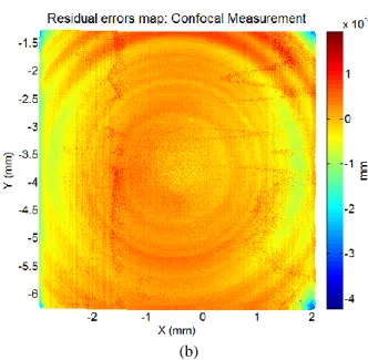
The experimental data show an equivalent accuracy among the two orthogonal distance-based fitting algorithms used which are also comparable to ICP in cases where the initial position of the elements to fit is relatively close (IP1 and IP2). The residual errors are illustrated in Fig. 4 for both tactile measurement fitting (Fig. 4a) and optical measruement fitting (Fig. 4b). Any of the algorithms returns the same error maps.

L-BFGS and LM perform faster than ICP in terms of computational time such as shown in Fig. 5. Nevertheless, all three algorithms are very low on memory storage and datasets of several millions of points can be processed using any of these algorithms. Although runtime is of the same order between LM and L-BFGS, the latter still performs a little faster than LM, and that, by a ratio of around 50%. For large volume datasets, the difference can be of some tens of seconds and therefore be critical for on-line metrology applications.

(a)

(b)

Fig. 4 Residual error maps. (a) Tactile measurement fitting, (b) Optical measurement fitting.

Fig. 5 CPU time performance of the L-BFGS, LM and ICP algorithms. Table4. The model parameters of the asphere after fitting both the tactile and the confocal datasets.

N = 500,000 Tactile dataset Confocal dataset

tp Rx (°) Ry (°) tx (mm) ty (mm) tz (mm) 0.0022868 0.0057522 0.1286046 -0.0510596 -2.989905E-4 0.0109687 11.99958 3.6542821 0.5042661 -0.4847707 mp c κ α2 α4 α6 α8 α10 4.969E-5 -1.0 0.0223669 -2.864146E-6 7.474612E-7 -3.375417E-8 5.373977E-10 2.192E-5 -1.0 0.0223392 -1.261943E-5 1.27085E-6 -3.160791E-8 2.737668E-10

"N. El-Hayek et al" / Procedia CIRP 00 (2014) 000–000

4.3. Discussion

L-BFGS, LM and ICP algorithms are tested on simulated datasets and they return similar results for the fitting on a given aspheric surface model. Since both algorithms are both Newtonian methods, applied on the same input datasets, it is logical that they converge to the same minimum. The algorithms are also tested on experimental datasets and the RMS and PV values are comparable. L-BFGS is slightly faster than LM and both perform faster than the classical ICP. However all three algorithms are very low on memory storage and can thus process very large datasets. Furthermore, all algorithms are invariant in regard to dataset size as they return the same residual errors when the number of points change. The adopted sampling strategy is that a reading is picked from the dataset but no filtration is applied. The Least-Squares minimization is not sensitive to point-set size when the latter has low uncertainty and contains a sufficient number of points. Tactile measurement is slower but more accurate than chromatic confocal measurement as the RMS and PV of the residual errors for tactile measurement are smaller, meaning that the tactile measurement is less noisy.

5. Conclusion and future work

This paper presents measurement and form characterization of aspheric surfaces. The comparison of optical and tactile measurements of an asphere using the LNE’s high precision profilometer is done based on a surface form characterization. LNE's primary profilometer, traceable to the SI meter definition is presented. Its architecture complies with the Abbe principle and its metrology loop is optimized. The performance and capability of the machine in the scope of aspheric lenses metrology are discussed.

Simulations and experiments have been conducted to test and compare the performance of three different algorithms for aspheric surface fitting. The results show that L-BFGS and LM perform faster than ICP in terms of computational time. Nevertheless, all three algorithms are very low on memory storage and datasets of several millions of points can be processed. Although runtime is of the same order between LM and L-BFGS, the latter still performs a little faster than LM, and is suitable for large number of data points.

Future research efforts will concentrate on improving the robustness and accuracy of the L-BFGS algorithm. Reference data set generation for the validation of metrological software for the characterization of aspheric surfaces will be also investigated.

Acknowledgements

This work is part of EMRP Joint Research Project-IND10 "Optical and tactile metrology for absolute form characterization" project. The EMRP is jointly funded by the EMRP participating countries within EURAMET and the European Union.

References

[1] Fang, F., Zhang, X., Weckenmann, A., Zhang, G., Evans, C., 2013. Manufacturing and measurement of freeform optics, in "CIRP

Annals-Manufacturing Technology".

[2] The EMRP website: http://www.emrponline.eu/

[3] Kaya, I., Thompson, K.P., Rolland, J.P., 2012. Comparative assessment of freeform polynomials as optical surface descriptions, in "Opt. Express", Vol.20, pp. 22683–22691. [4] Chen, Z., Guo, Z., Mi., Q., Yang. Z., Bai, R., 2009. Research of

fitting algorithm for coefficients of rotational symmetry aspheric lens, in Proc. SPIE 7283, 4th _{Intl. Symp. on Adv. Opt. Manuf. and}

Test. Tech.: Opt. Test and Meas. Tech. and Equip., Vol. 7283

[5] Moré, J., 1978. The Levenberg-Marquardt algorithm: implementation and theory, in "Numerical analysis", Springer,

pp. 105-116.

[6] Aceves-Campos, H., 1998. Profile identification of aspheric lenses, in "Applied Optics", Vol. 37 (34), pp. 8149-8150.

[7] Zhang, Z., 1997. A tutorial with application to conic fitting, in

"Image and vision computing", Vol. 15 (1), pp. 59-76.

[8] Sun, W., McBride, J-W., Hill, M., 2010. A new approach to characterizing aspheric surfaces, in "Precision Engineering", Vol. 34(1), 2010, pp.171-179.

[9] Park, H., 2004. A solution for NURBS modelling in aspheric lens manufacture, in "The Intl. J. of Adv.Manuf. Tech.", Vol. 23 (1-2), pp.1-10.

[10] Forbes, A. B., 1993. Generalised regression problems in metrology. Numerical Algorithms, Vol. 5(10), pp. 523-533. [11] Shakarji, C., 1998. Least-Squares fitting algorithms of the NIST

algorithm testing system, in "J. of research of the Nat. Inst. Of

Std. and Tech.", Vol. 103, pp. 633-641.

[12] Lancaster, P., 1966. Error analysis for the Newton-Raphson method, in "Numerische Mathematik", Vol. 9 (1), pp. 55-68. [13] Süli, E., Mayers, D., 2003. An introduction to numerical analysis,

in "Cambridge University Press", 2003.

[14] Transtrum, M. K., & Sethna, J. P. (2012). Improvements to the Levenberg-Marquardt algorithm for nonlinear least-squares minimization.. arXiv preprint arXiv:1201.5885.

[15] Speer, T., Kuppe, M., Hoschek, J., 1998. Global reparametrization for curve approximation, in "Computer Aided Geometric Design", Vol. 15 (9), pp. 869-877.

[16] Nocedal, J., Wright, S., 1999. Numerical Optimization, in

"Springer New York", Vol. 2, 1999.

[17] Nocedal, J., 1980. Updating quasi-Newton matrices with limited storage, in "Mathematics of computation", Vol. 35 (151), pp. 773-782.

[18] Liu, D., Nocedal, J., 1989. On the limited memory BFGS method for large scale optimization, in "Mathematical programming", Vol. 45 (1-3), pp. 503-528.

[19] Zheng, W., Bo. P., Liu, Y., Wang, W., 2012. Fast B-Spline curve fitting by L-BFGS, in "Computer Aided Geometric Design", Vol. 29 (7), pp. 448-462.

[20] Zhang, M., 2011. Discrete shape modeling for geometrical product specifications: Contributions and applications to Skin Model simulation. Ph.D. thesis, Ecole Normale Superieure de Cachan, France.

[21] El-Hayek, N., Nouira, H., Anwer, N., Damak, M., Gibaru, O., 2013. Reconstruction of freeform surfaces for metrology, in

"Proc. Of the 14th _{Intl. Conf. on Metrol. and Prop. of Eng. Surf.",}

[22] Pomerlau, F., Colas, F., Siegwart, R., Magnenat, S., 2013. Comparing ICP variants on real-world data sets, in "Autonomous

Robots", Vol. 34 (3), pp. 133-148.

[23] Zhao, H., Anwer, N., Bourdet, P., 2013. Curvature-based Registration and Segmentation for Multisensor Coordinate Metrology, in "Procedia CIRP", Vol. 10, pp. 112-118.

[24] Halina, N., Chuchro, Z., 2009. Some comments on reference data set generation in passing, in XIX IMEKO World Congress Fundamental and Applied Metrology, Lisbon, Portugal. [25] Jiang, X., Zhang, X., Scott, P., 2010. Template matching of

freeform surfaces based on orthogonal distance fitting for precision metrology, in "Measurement Science and Technology", Vol. 21 (4), 10p.

[26] Mandelbrot, B., Ness, JW., 1968. Fractional Brownian Motions, Fractional Noise and applications, in "SIAM Review”, Vol.10, pp. 422–437.