STATISTICAL PROPERTIES OF DAILY RETURNS: EVIDENCE
FROM EUROPEAN STOCK MARKETS
Corhay A(1)(2), Tourani Rad A(1) (1)University of Liege, Belgium
(2)University of Limburg, the Netherlands Introduction
An increasing number of empirical studies, starting with Mandelbrot (1963) and Fama (1965), have shown that time series of financial asset returns tend to be serially uncorrected over time but not independent. Although it is generally accepted that distributions of stock returns are leptokurtic and skewed, there is no unanimity regarding the best stochastic return generating model to capture these empirical characteristics. For an extensive list of studies in this area, see Bookstaber and McDonald (1987).
One of the recently proposed class of return generating processes in the literature is the class of autoregressive conditional heteroskedastic models introduced by Engle (1982) and its generalized versions by Bollerslev (1986 and 1987). Empirical studies have shown indeed that such processes are successful in modelling various time series. See, for example, in the context of foreign exchange markets, Baillie and Bollerslev (1989) and Hsieh (1989), and in the context of stock markets, French et al. (1987), Akgiray (1989) and Baillie and De Gennaro (1990).
As far as stock markets are concerned, this class of models has mainly been applied to large American markets such as the New York Stock Exchange, e.g. by Akgiray (1989), and also to the London Stock Exchange by Poon and Taylor (1990). The objective of this paper is to investigate whether such models can adequately describe stock price behaviour in European capital markets which are generally much smaller and thinner than the American ones. To that end, we have selected the following five countries: France, Germany, Italy, the Netherlands and the United Kingdom. The study of stock price behaviour in these markets is interesting because it can provide further evidence in favour of or against the use of this type of model to describe stock price behaviour.
The remainder of the paper is organised as follows. The next section presents the data, and descriptive statistics and other statistical properties of the return series of all five countries. In the third section, the class of autoregressive conditional heteroskedastic models is discussed and applied to these return series. Conclusions and implications are then presented in the final section.
Data and statistical findings The Data
The indices of five European stock markets were collected from DATASTREAM for the period 1/1/1980 to 30/9/1990. They are indices for France (CAC General), Germany (Commerzbank), Italy (Milan Banca), the Netherlands (ANP-CBS general) and the UK (FT All-Shares). All indices, except the one for the Netherlands, are value weighted. The ANP-CBS index is in fact a weighted average of a number of sector indices. A complication we faced is that some of these indices are not adjusted for dividends. This is not ideal from a theoretical point of view, but they are the best available indices for the period under consideration. However, since the objective of this paper is to model non-linear dependencies in stock returns, we would expect that dividend adjustment would not affect our results. This point has already been discussed in French et al. (1987) and Poon and Taylor (1990). Both studies have shown that the dividend adjustment has little or no effect on the estimates of their models. The daily returns of the market indices in our sample are continuously compounded returns. They are calculated as the difference in natural logarithm of the closing index value for two consecutive trading days, Rt= log(Pt) — log(Pt-1). The number of returns for each country can be found in Table 1.
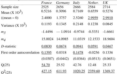
Table 1 presents a range of statistics for the five indices. They are: mean, variance, skewness and kurtosis. It can be observed that there are differences across the countries regarding the mean and the variance of the return series. Under the assumption of normality m3and m4, the standard measures of
skewness and kurtosis, have asymptotic distributions N(0,6/T) and Ar(3,24/T), respectively, where T is the sample size. All distributions are negatively skewed, indicating that they are non-symmetric. Furthermore, they all exhibit high levels of kurtosis, which indicates that these distributions have fatter tails than normal distributions. The Kolmogorov-Smirnov D-statistic to test the null hypothesis of normality has also been calculated, and it rejects the normality assumption at the significance level of one per cent in all cases. The results confirm the well known fact that daily stock returns are not normally distributed, but are leptokurtic and skewed.
Table 1 Sample Statistics on Daily Return Series*
France Germany Italy Nether. UK
Sample size 2525 2656 2666 2584 2714 Mean (X 1O3) 0.5216 0.3096 0.7169 0.6559 0.5276 ((mean = 0) 2.4000 1.3757 2.5260 2.9959 2.9910 Variance (X 103) 0.1193 0.1345 0.2148 0.1238 0.0845 m3 -1.4496 — 1.0914 -0.9744 -0.5351 -1.6661 m4 15.0024 14.0985 11.0319 12.1533 18.9604 D-statistic 0.0830 0.0674 0.0941 0.0591 0.0467
First order autocorrelation 0.1395 0.0318 0.1478 -0.0256 0.1336
(0.0307) (0.0442) (0.0364) (0.0513) (0.0651)
Q(25) 54.70 25.52 42.76 12.48 25.33
Q2(25) 427.15 611.93 1020.25 2359.60 1369.37
Note: * t-statistics significant at the one per cent level are underlined. Numbers in parentheses are heteroskedasticity-consistent standard errors.
Tests of Autocorrelation
Our objective here is to investigate whether stock returns can be represented by a random walk, that is, if returns Rtare independently distributed random variables with expectation E(Rt) = 0. It should be
noted that market efficiency does not require return series to be distributed independently. Fama (1970) showed that a market is efficient if the return process is a martingale, i.e. E(Rt) = 0.
The Box-Pierce test statistic adjusted for heteroskedasticity Q(k), as suggested by Diebold (1987), up to lag 25 is calculated and presented in Table 1. This is a joint test of the null hypothesis that the first k autocorrelation coefficients are zero. Under the null hypothesis, the adjusted Box-Pierce statistic, Q(k) =∑ki=1ρ(i)/S(i))2, follows a ch i-square distribution with k degrees of freedom, where ρ(i) is the zth
autocorrelation. S(i) is a heteroskedasticity-consistent estimate of the standard error for the zth sample autocorrelation coefficient, √l/n(1 +γR2(i)/σ4), where γR2(i) is the ith sample autocovariance of the square data and σ is the sample standard deviation of the data. The values of Q(25) are significant at the
one per cent level for France and at the five per cent level for Italy. This suggests that, after adjusting for heteroskedasticity, there remains some long term dependency in the series of returns for these two countries.
Table 1 also presents Q2(25) which is the Box-Pierce statistic based on the squared return series. Under the null hypothesis of conditional homoskedas-ticity, the statistic Q2(k) has an asymptotic chi-square distribution with k degrees of freedom. The null hypothesis is strongly rejected at the one per cent significance level for all countries.
Autoregressive Models
0.0318 for Germany, 0.1478 for Italy, -0.0256 for the Netherlands and 0.1336 for the UK. These are significant at the one per cent level for France and Italy, and at five per cent for the UK, indicating that the daily index returns for these countries are first order serially correlated. The rather low and insignificant coefficients of the first order serial correlation coefficient for German and Dutch indices might be explained by the important weight of a few large, frequently and highly traded firms, of which returns are not autocorrelated, in the calculation of the indices.
One way to generate an uncorrelated series for France, Italy and the UK is to apply an AR(1) model, that is:
(1)
The estimates of the above regression model for each country are presented in Table 2. In order to observe the behaviour of the residuals εtobtained from equation (1), we applied the same tests as for
the return series. The first order,autocorrelation coefficient for all countries is not significantly different from zero.
Table 2 The Autoregressive Model*
France Italy UK
Estimates of the Model
0.0004 0.0006 0.0004 2.1398 2.1611 2.6302 0.1395 0.1478 0.1337 7.0876 7.7131 7.0259 F-statistic 50.235 59.4927 49.3639 R2 0.0195 0.0218 0.0179 Fuller's test 2172.6 2272.0 2351.2
Statistics on Daily Residuals Series
Sample size 2524 2665 2713 Mean (x 1O3) 0.0000 0.0000 0.0000 ((mean = 0) 0.0000 0.0000 0.0000 Variance (x lO3) 0.1166 0.2101 0.0829 m3 -1.3572 -0.7871 -1.3008 m4 15.5796 11.3745 16.2624
First order autocorrelation -0.0087 0.0098 -0.0046
(0.0339) (0.0411) (0.0660)
Q(25) 27.40 26.12 16.05
Q2(25) 434.09 968.82 1930.51
Notes: * t-statistics significant at the one per cent level are underlined. Numbers in parentheses are heteroskedasticity-consistent standard errors.
Furthermore, the insignificant values of Q.(25) indicate that the AR(1) transformation of the returns provides an uncorrected series of residuals.
The estimates of are statistically significant at the one per cent level and the Dickey-Fuller test for a unit root indicates that the are significantly less than one. The three series of returns appear to follow a stationary random walk. As far as distributions of residuals are concerned, it appears that they are still leptokurtic and skewed in comparison with the normal distribution. Furthermore, the values of Q (25) decisively reject the null hypothesis of conditional homoskedasticity.
The excess kurtosis observed in both returns and residuals series of the five countries in our sample can be related to conditional heteroskedasticity, that is, its presence can be due to a time varying pattern of the volatility.
Conditional heteroskedastic models
example, by Morgan (1976) and Giaccoto and Ali (1982). But while they focused on unconditional heteroskedasticity, in this paper we use Engle's Autoregressive Conditional heteroskedastic (ARCH) model which focuses on conditional volatility movements. It is interesting to note that, according to Diebold et al. (1988), the presence of the ARCH effect appears to be generally independent of unconditional heteroskedasticity.
(G)ARCH Models
The ARCH process imposes an autoregressive structure on the conditional variance which permits volatility shocks to persist over time. It can therefore allow for volatility clustering, that is, large changes are followed by large changes, and small by small, which has long been recognized as an important feature of stock returns behaviour. In the context of the original model, the conditional error distribution is normal, with a conditional variance that is a linear function of past squared innovations. The model, denoted by ARCH(p), is the following:
(2)
with p > 0; αi > 0, i = 0, . . ., p,
and where is the information set of all information through time t, and the etare the returns for
Germany and the Netherlands and the residuals of an AR(1) model for the other three countries. An important extension of the ARCH model is the Generalized Autoregressive Conditional
Heteroskedasticity (GARCH) process of Bollerslev (1986), denoted by GARCH(p,q). In this model, the linear function of the conditional variance includes lagged conditional variances as well. Each country's returns volatility depends on past period squared errors and its own past conditional variances. The equation (2) in the case of a GARCH model becomes:
(3)
where also q ≥ 0 and βj> 0,j = 1, . . ., q. The GARCH(p,q) model reduced to an ARCH(p) for q = 0.
Even though GARCH models with conditional normal distribution allow unconditional error distributions to be leptokurtic, they might not fully explain the high level of kurtosis in observed distributions of return series. It has been suggested in the literature that the assumption of a leptokurtic conditional distribution in GARCH models might be more appropriate since such distribution can better account for the level of kurtosis observed in financial data than does the normal conditional distribution. This allows a distinction between conditional heteroskedasticity and a conditional
leptokurtic distribution, either of which could generate the fat tailedness observed in the data. Different conditional leptokurtic distributions have been applied in the literature (Baillie and Bollerslev, 1989; and Hsieh, 1989). And it is generally found that the t-distribution, originally proposed by Bollerslev (1987), performs better than other distributions.
In conditional heteroskedastic models, the stability condition of the variance process requires that the sum of the estimated parameters, i.e. ∑pi=1αi + ∑qj=1βjwhich measures the persistence of the volatility,
to be less than one. If this sum is equal to one, the process becomes an integrated GARCH or IGARCH process (Engle and Bollerslev, 1986). Such integrated processes imply the persistence of a forecast of the conditional variance over all future horizons and also an infinite variance of the unconditional distribution of et.
Estimation and Testing
All (G)ARCH models are estimated using a FORTRAN program which employs the nonlinear optimization technique of Berndt et al. (1974) to compute maximum likelihood estimates. Given the return series and initial values of ε1 and h1for 1 = 0, . . . , r and with r = max(p,q), the log-likelihood
function we have to maximize for a GARCH(p,q) model with normal distributed conditional errors is the following:
(4) where T is the number of observations;
ht, the conditional variance, is defined by equations (2) and (3) for the ARCH and GARCH models
respectively;
εt2, are the residuals obtained from the appropriate model for the country under consideration.
In the case of t-distributed conditional errors, the loglikelihood function for this model, denoted hereafter by GARCH(p,q) — t, is:
(5)
where Γ(*) denotes the gamma function and is the degrees of freedom. If the t-distribution approaches a normal distribution, but for the
^-distribution has fatter tails.
In order to test for the relative fit of the various models, the likelihood ratio test (LR) will be
employed, where and
denote the maximized likelihood functions estimated under the null hypothesis and the alternate hypothesis. Under the null hypothesis LR is chi-square distributed with degrees of freedom equal to the difference in the number of parameters under the two hypotheses. Moreover, to distinguish between an improvement in the likelihood function due to a better fit and an improvement due to an increase in the number of parameters, we also calculate Schwarz's order selection criterion,where K is the number of parameters in the model. According to this criterion, the model with the lowest SIC value fits the data best.
Empirical Results
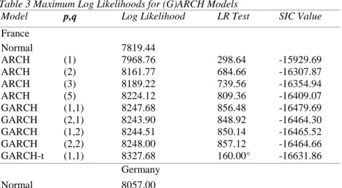
Several (G)ARCH models were estimated using different combinations of p and q for each of the five countries in our sample. The values of p and q and the corresponding maximized log-likelihood for each (G)ARCH model as well as that obtained when an unconditional normal distribution is imposed on the data, are presented in Table 3 by country. Pure ARCH(p) processes of order up to five were first fitted to the data. The LR test, which compares the fitness of an ARCH(p) model with that of an unconditional normal distribution, are all statistically significant at the one per cent level, indicating that all ARCH(p) models fit the data better than the normal distribution. As for the GARCH(p,q) models, they were estimated for p = 1,2 and q = 1,2. The values of LR tests again indicate that these models fit the data better than the unconditional normal distribution.
Table 3 Maximum Log Likelihoods for (G)ARCH Models
Model p,q Log Likelihood LR Test SIC Value
France Normal 7819.44 ARCH (1) 7968.76 298.64 -15929.69 ARCH (2) 8161.77 684.66 -16307.87 ARCH (3) 8189.22 739.56 -16354.94 ARCH (5) 8224.12 809.36 -16409.07 GARCH (1,1) 8247.68 856.48 -16479.69 GARCH (2,1) 8243.90 848.92 -16464.30 GARCH (1,2) 8244.51 850.14 -16465.52 GARCH (2,2) 8248.00 857.12 -16464.66 GARCH-t (1,1) 8327.68 160.00° -16631.86 Germany Normal 8057.00
ARCH (1) 8221.67 329.34 -16435.46 ARCH (2) 8302.18 490.36 -16588.59 ARCH (3) 8406.06 698.12 -16788.47 ARCH (5) 8437.42 760.84 -16835.42 GARCH (1,1) 8446.38 778.75 -16876.99 GARCH (2,1) 8436.32 758.64 -16848.99 GARCH (1,2) 8439.41 764.82 -16855.17 GARCH (2,2) — GARCH-t (1,1) 8554.01 215.26° -17084.37 Italy Normal 7465.00 ARCH (1) 7636.40 342.80 -15264.91 ARCH (2) 7838.05 746.10 -15660.32 ARCH (3) 7886.53 843.06 -15749.39 ARCH (5) 7915.62 901.24 -15791.80 IGARCH (1,1) 7905.85 881.70 -15795.22 GARCH (2,1) — GARCH (1,2) — GARCH (2,2) — GARCH-t (1,1) 8071.02 330.34° -16118.38 The Netherlands Normal 7944.42 ARCH (1) 8100.35 331.86 -16192.84 ARCH (2) 8197.61 506.38 -16379.51 ARCH (3) 8211.94 535.04 -16400.31 ARCH (5) 8247.88 606.92 -16456.47 GARCH (1,1) 8251.36 613.88 -16487.01 GARCH (2,1) 8237.99 587.14 -16452.41 GARCH (1,2) — GARCH (2,2) — GARCH-.t (1,1) 8307.17 111.62° -16590.77
Model p,q Log Likelihood LR Test SIC Value
The UK Normal 8864.31 ARCH (i) 9065.35 402.08 -18122.79 ARCH (2) 9126.77 524.92 -18237.73 ARCH (3) 9144.31 560.00 -18264.90 ARCH (5) 9152.34 576.06 -18265.15 GARCH (1.1) 9140.74 552.86 -18265.67 GARCH (2,1) 9126.17 523.72 -18228.62 GARCH (1.2) 9135.76 542.90 -18247.80 GARCH (2,2) — GARCH-t (1,1) 9214.97 148.76° -18406.22
Notes:— indicates where the optimization routine failed.
° The null hypothesis is that conditional errors of GARCH(1,1) model are normally distributed.
Italy excepted, SIC values are the lowest for the GARCH(1,1), indicating that this model generally outperforms other (G)ARCH models, as can be seen in Table 3. Concerning Italy, the unrestricted GARCH(1,1), i.e. without imposing any restriction on the α1 + β1, was non-stationary. Therefore, we
proceeded to estimate an IGARCH(1,1) model for this country, which on the basis of the LR test and the SIC value fits best, as reported in Table 3.
Finally, we estimate the GARCH(1,1) model assuming that conditional errors follow a t-distribution instead of a normal one. It can be observed that all values of the log-likelihood are substantially larger than those for the GARCH(1,1) model with normally distributed conditional errors. All likelihood ratio tests for the null hypothesis, i.e. conditional errors are normally distributed, and are statistically significant, indicating that a GARCH-t(1,1) fits the data better.
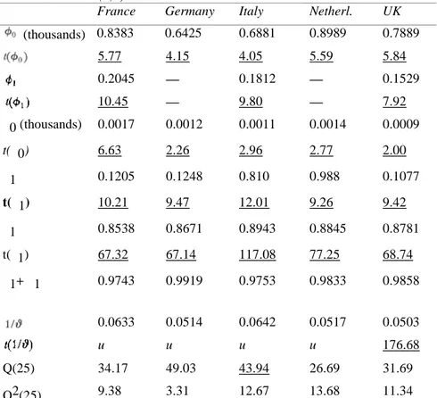
Table 4 contains the results of fitting this process to the return series of France, Germany, Italy, the Netherlands and the UK. All estimated coefficients, except α0 for the UK, are statistically significant at
the one per cent level. We observe that estimated values of the inverse of the degrees of freedom parameter in the t-distribution, range from 0.0503 to 0.0642 and are highly statistically significant.
As for the stationarity of the variance process, it can be observed that α1+ β1 are respectively 0.9743,
0.9919, 0.9753, 0.9833 and 0.9858 for France, Germany, Italy, the Netherlands and the UK. They are all less than unity, indicating no violation of the stability condition, i.e. the GARCH-t(1,1) is second order stationary and the second moment exists for each country. These sums are, however, rather close to one, which indicates a long persistence of shocks in volatility.
Table 4 GARCH-t (1,1) Estimates*
France Germany Italy Netherl. UK
(thousands) 0.8383 0.6425 0.6881 0.8989 0.7889 5.77 4.15 4.05 5.59 5.84 0.2045 — 0.1812 — 0.1529 10.45 — 9.80 — 7.92 α0 (thousands) 0.0017 0.0012 0.0011 0.0014 0.0009 t(α0) 6.63 2.26 2.96 2.77 2.00 α1 0.1205 0.1248 0.810 0.988 0.1077 t(α1) 10.21 9.47 12.01 9.26 9.42 β1 0.8538 0.8671 0.8943 0.8845 0.8781 t(β1) 67.32 67.14 117.08 77.25 68.74 α1+ β1 0.9743 0.9919 0.9753 0.9833 0.9858 0.0633 0.0514 0.0642 0.0517 0.0503 u u u u 176.68 Q(25) 34.17 49.03 43.94 26.69 31.69 Q2(25) 9.38 3.31 12.67 13.68 11.34
Notes: * t-statistics significant at the one per cent level are underlined. u indicates very large significant t-values.
All values of the Pierce statistic on the standardized residuals, Q(25), and all values of the Box-Pierce statistic on the squared residuals, Q2(25), do not reveal any first and second order dependence, with the exception of Germany in the case of which there remains some first order dependence. This confirms that the GARCH-t(1,1) model fits the return series in our sample reasonably well. Each country's returns volatility depends on last period's squared error and its own past conditional variance.
Conclusion and implications
Our results clearly indicate that conditional heteroskedasticity is a prime feature of daily returns behaviour of five European equity indices. They exhibit non linear dependence that cannot be captured by the random walk model. The class of autoregressive conditional heteroskedastic models is generally consistent with the stochastic behaviour of these return series. The evidence presented in this paper reveals that the GARCH-t(1,1), i.e. a GARCH model with conditional errors that are t-distributed, fits the data best. Thus our results confirm that this class of models is also appropriate for studying the behaviour of stock returns on smaller equity markets.
Such empirical evidence can have important implications for research in finance. GARCH models may, for example, be used to analyse the relationships between volatility and expected returns. In the Capital
Asset Pricing Model, the expected return or risk premium can be influenced by the conditional second moment of returns. As for empirical research, event study methodology, for example, assumes homoskedasticity. As it is not the case, one can cast doubt on the way abnormal returns are calculated and consequently interpreted. Volatility estimation is also an important feature for pricing derivative securities. GARCH models can indeed provide better forecasts of volatility than the usual historical estimates and lead to improved valuation models.
Note
1 This program has been developed by Ken Kroner at the University of California. It was kindly provided to us by Robert Engle.
References
Akgiray, V. (1989), 'Conditional Heteroskedasticity in Time Series of Stock Returns: Evidence and Forecasts', Journal of Business, Vol. 62, No. 1 (January 1989), pp. 55-80.
Baillie, R.T. and T. Bollerslev (1989), 'The Message in Daily Exchange Rates: A Conditional-Variance Tale', Journal of Business & Economic Statistics, Vol. 7, No. 3 (July 1989), pp. 297-305.
_______ and R.P. De Gennaro (1990), 'Stock Returns and Volatility', Journal of Financial and Quantitative Analysis, Vol. 25, No. 2 (June 1990), pp. 203-214.
Berndt, E.K., B.H. Hall, R.E. Hall and J.A. Hausman (1974), 'Estimation and Inference in Nonlinear Structural Models', Annals of Economies and Social Measurement, Vol. 4 (1974), pp. 653-665.
Bollerslev, T. (1986), 'Generalized Autoregressive Conditional Heteroskedasticity', Journal of Econometrics, Vol. 31 (April 1986), pp. 307-327.
_______(1987), 'A Conditionally Heteroskedastic Time Series Model for Security Prices and Rates of Return Data', Review of Economics and Statistics, Vol. 59 (August 1987), pp. 542-547.
Bookstaber, R. and J. McDonald (1987), A General Distribution for Describing Security Price Returns, Journal of Business, Vol. 60, No. 3 (July 1987), pp. 401-424.
Diebold, F.X. (1987), 'Testing for Serial Correlation in the Presence of ARCH', Proceedings from the American Statistical Association, Business and Economic Statistics Section (1987), pp. 323-328.
_______, J. Im and C.J. Lee (1988), 'Conditional Heteroskedasticity in the Market', Finance and Economics Discussion Series, 42, Division of Research and Statistics, Federal Reserve Board, Washington DC (1988).
Engle, R. (1982), 'Autoregressive Conditional Heteroskedasticity with Estimates of the Variance of UK Inflation', Econometrica, Vol. 50, No. 4 (July 1992), pp. 987-1008.
Fama, E.F. (1965), 'The Behavior of Stock Market Prices', Journal of Business, Vol. 38, No. 1 (January 1965), pp. 34-105.
_______(1970), 'Efficient Capital Markets: A Review of Theory and Empirical Work', Journal of Finance, Vol. 25 (May 1970), pp. 383-417.
French, K.R., G.W. Schwert and R.F. Stambaugh (1987), 'Expected Stock Returns and Volatility', Journal of Financial Economics, Vol. 19 (September 1987), pp. 3-29.
Giaccoto, C. and M.M. AH (1982), 'Optimal Distribution Free Tests and Further Evidence of Heteroskedasticity in the Market Model', Journal of Finance, Vol. 37, No. 4 (September 1982),
pp. 1247-1257.
Hsieh, D.A. (1989), 'Modelling Heteroskedasticity in Daily Foreign-Exchange Rates', Journal of Business & Economic Statistics, Vol. 7, No. 3 (July 1989), pp. 307-317.
Mandelbrot, B. (1963), 'The Variation of Certain Speculative Prices', Journal of Business, Vol. 36, No. 3 (July 1963), pp. 394-419.
Morgan, I. (1976), 'Stock Prices and Heteroskedasticity', Journal of Business, Vol. 49, No. 4 (October 1976), pp. 496-508.
Poon, S.H. and S. Taylor (1990), 'Stock Returns and Volatility: An Empirical Study of the UK Stock Market', paper presented at the 17th European Finance Association meeting, Athens (1990).
Schwarz, G. (1978), 'Estimating the Dimension of a Model', the Annals of Statistics, Vol. 6, No. 2 (1978), pp. 461-464.