Acoustic Characterization of a Stationary Field Synchronous Motor
By
E. C. Woodward, Jr.
Bachelor of Electrical Engineering, Vanderbilt University, 1995
Master of Science, School of Electrical Engineering, Georgia Institute of Technology, 1996 SUBMITTED IN PARTIAL FULFILLMENT
OF THE REQUIREMENTS FOR THE DEGREES OF MASTER OF SCIENCE,
NAVAL ARCHITECTURE AND MARINE ENGINEERING, and
MASTER OF SCIENCE,
ELECTRICAL ENGINEERING AND COMPUTER SCIENCE at the
MASSACHUSETTS INSTITUTE OF TECHNOLOGY, August, 2001
L~er;Aem~\e
~OQI@ E.C. Woodward Jr., 2001. All rights reserved. Permission is granted to MIT for reproduct distribution in whole or in part.
Signature of Author: ,, t. Certified By: I
V7
Certified By: Accepted By:. IDepartments of Ocean Engineering August 10, 2001
James L. Kirtley Professor of Electrical Engineering and Computer Science Thesis Supervisor
Clifford Whitcomb Research Scientist Thesis Supervisor
Arthwr C.-Smith
Chairman, Committee on Graduate Students Department of Electrical Engineering and Computer Science Accepted By:
Henrik Schmidt SSACHLJSETTS IN TITUTE Hni cmd
OF TECHNOLOGY hairman, Committee on Graduate Students Department of Ocean Engineering
Acoustic Characterization of a Stationary Field Synchronous Motor
By
E. C. Woodward, Jr.
Submitted to the Department of Ocean Engineering
and the Department of Electrical Engineering and Computer Science on August 10, 2001 in Partial Fulfillment of the Requirements for the Degrees of Master of Science, Naval
Architecture and Marine Engineering, and Master of Science, Electrical Engineering and Computer Science, Respectively.
Abstract. The stationary field synchronous motor (SFSM) has been described and analyzed previously. This machine usually consists of a stationary, direct current field winding and a rotating, alternating current armature winding. The field winding is super-conducting. This topology presents certain advantages and disadvantages. One of the greatest theoretical advantages is reduced acoustic emission. The precise nature of such reductions has not been considered in previous work. We investigate the gross acoustic signature of a notional stationary field synchronous motor utilized as a marine propulsion motor in a naval combatant using the following methodology: (1) model the forces (harmonic by harmonic) of electromagnetic origin using solutions of the two dimensional Laplace Equation arising from the scalar potential of a magnetic field, (2) Develop a force spectrum based upon this
modeling, (3) Develop appropriate acoustic transfer functions describing the acoustic
propagation of the machine components, equipment mounting structures, and other pertinent items in the machine-to-sea sound conduction path, (4) Apply the force spectrum to the acoustic transfer function(s), and (5) obtain a meaningful far-field acoustic signature due to the SFSM.
Thesis Advisor: James L Kirtley, Jr.
ACKNOWLEDGEMENTS
I wish to thank Professor James L. Kirtley, Jr. for his guidance throughout my research work. This work was made possible by the sponsorship of the United States Navy through the MIT
Table of Contents
G L O SSA R Y O F T E R M S... 6
L IST O F F IG U R E S ... 8
L IST O F T A B L E S... 9
CHAPTER ONE. INTRODUCTORY MATTER ... 10
1.0 IN T R O D U C T IO N ... 10
1.1 SFSM D ISA D V A N TA G ES... 10
1.2 SFSM A D V A N TA G E S ... 10
1.3 THE GENERAL HYPOTHESIS... 10
1.4 ACOUSTIC SOURCES IN ELECTRICAL MACHINERY ... 11
1.5 PROBLEM FORMULATION... 12
CHAPTER TWO. FORCE CHARACTERIZATION AND MODELING ... 13
2.0 SFSM CHARACTERIZATION AND MODELING ... 13
2.1 PRO AND CON OF THE SFSM... 13
2.2 MOTOR TOPOLOGY SELECTION ... 13
2.3 CR U D E M O TO R SIZIN G ... 14
2.4 THE NATURE OF HARMONICS WITHIN THE SFSM ... 16
2.4.1 CORE SATURATION HARMONICS... 16
2.4.2 SLOT SATURATION HARMONICS ... 16
2.4.3 TIM E H A R M O N IC S ... 17
2.4.4 SPA C E H A R M O N IC S ... 17
2.5 MACHINE TOPOLOGY AND FIELD MODELING ... 18
2.6 FO R C E A N A L Y SIS ... 19
2.6.1 MAGNETIC FIELD INTENSITY DUE TO THE SUPERCONDUCTING MOTOR FIELD W IN D IN G S ... 19
2.6.2 MAGNETIC FIELD INTENSITY DUE TO THE MOTOR ARMATURE WINDINGS... 21
2.6.3 MAGNETIC FIELD DUE TO TERMINAL CURRENT POWER SUPPLY TIME H A R M O N IC S ... 2 1 2.6.4 THE COMPOSITE MAGNETIC FIELD INTENSITY ... 23
2.6.5 MAGNETIC FIELD OF INTEREST IN MOTOR SHELL DEFLECTIONS... 24
2.6.6 FORCE ON THE MOTOR SHELL ... 25
2.6.6.1 DEVELOPMENT OF THE MAXWELL STRESS TENSOR APPROACH ... 25
2.6.6.2 SIMPLIFICATION OF THE FORCE INTEGRAL INTEGRAND ... 27
2.6.7 FO R C E S O F IN TER EST ... 27
2.6.7.1 FORCES ARISING FROM HARMONIC TO FUNDAMENTAL INTERACTIONS ... 28
2.6.8 CONCLUSIONS REGARDING FORCES ON THE SFSM STATOR ... 29
CHAPTER THREE. MOTOR SHELL STRUCTURAL ANALYSIS ... 30
3.0 DEVELOPMENT OF THE ACOUSTIC MODEL ... 30
3.1 STRUCTURAL CHARACTERIZATION OF THE MOTOR SHELL ... 31
3.1.1 MOTOR SHELL RESONANT FREQUENCIES AND MODES ... 32
3.1.1.1 DETAILS OF THIN SHELL EQUATIONS ... 32
3.1.1.2 MODES AND RESONANT FREQUENCIES OF THE MOTOR SHELL ... 33
3.1.2 AVOIDANCE OF RESONANCE ... 35
3.2 SHELL DEFLECTIONS VIA STATIC APPROACH ... 36
3.3 SHELL VIBRATION VELOCITIES ... 39
3.4 SOUND RADIATION FROM THE SHELL ... 40
3.4.1 IDEAL SOUND RADIATOR THEORY ... 40
3.4.2 SPHERICAL RADIATOR EQUATIONS ... 40
CHAPTER FOUR. ACOUSTIC MODELING ... 42
4.0 DEVELOPMENT OF THE ACOUSTIC SPECTRUM OF THE SFSM... 42
4.1 COMBINING THE VIBRATION VELOCITIES AND THE ACOUSTIC ANALYSIS TO OBTAIN A THEORETICAL ACOUSTIC SIGNATURE... 42
4.2 ACOUSTICS SIGNATURE OF THE SFSM SHELL... 42
5.0 ACOUSTIC COMPARISON OF SFSM WITH A CONVENTIONAL AC SUPERCONDUCTING
M O T O R ... 44
5.1 CONVENTIONAL MACHINE DESCRIPTION... 44
5.2 FORCES OF INTEREST IN THE CONVENTIONAL MACHINE ... 44
5.3 STRUCTURAL ANALYSIS OF CONVENTIONAL MACHINE ... 45
5.4 THEORETICAL ACOUSTIC SIGNATURE OF A CONVENTIONAL MOTOR SHELL ... 46
5.5 COMPARISON OF SIGNATURES... 47
CHAPTER SIX. CONCLUSIONS AND RECOMENDATIONS... 48
6.0 C O N C L U SIO N S ... 48
6.1 R EC O M EN D A T IO N S ... 48
APPENDIX ONE, MOTOR SIZING CALCULATIONS... 50
APPENDIX TWO, ELECTROMAGNETIC FORCE CALCULATIONS ... 51
APPENDIX THREE, STRUCTURAL RESONANT FREQUENCIES... 53
APPENDIX FOUR, STATIC DEFLECTION CALCULATIONS ... 55
APPENDIX FIVE, RADIATED ACOUSTIC POWER CALCULATIONS ... 57
APPENDIX SIX, VERIFICATION OF ZERO TRIPLEN HARMONICS ... 58
Glossary of Terms
Subscripts a armature f field i inner o outer r radial coordinate s stator z axial coordinate 0 azimuthal coordinate 0 fundamental 1.. harmonic number Symbols T vector potential (D scalar potential<P phase shift angle, in degrees
p material density, in kilograms per cubic meter Bf main field magnetic flux density, in Teslas
Ba armature magnetic flux density, in Teslas
H magnetic field intensity, in Amperes per meter I current, in Amperes
J current density, in amperes per square meter K surface current density, in amperes per meter k wave number
1 length, in meters
la armature active length, in meters L inductance, in Henrys
N number of turns R radius, in meters t thickness
V Voltage, in volts
power factor angle, in degrees
C> angular frequency, in inverse seconds
xd synchronous reactance, per unit
p number of poles P pressure, in Pascals
v vibrational velocity, in meters per second
Pal reference pressure at one meter from radiator service T torque, in Newton meters
t C AC dS M F
Q
V E 6 T p K h k KD Xflugge fflugge A Z z D C Ta Tb tsshear stress, in Newtons per square meter Capacitance, in Farads
area of conductor, in square meters differential path length
mass, in kilograms
acceleration, in meters per second squared force, in Newtons
Force per Unit Length, newtons per meter Poisson's Ratio, a unitless constant Elastic Modulus, in Pascals
deflection, in meters machine shear, in Pascals density, in kg per cubic meter shell mode parameter
wave number, inverse meters shell thickness, in meters structural resonance parameter Flugge Shell Resonance Parameter
Flugge Shell Natural Frequency Parameter Flugge Shell Coefficient
Natural Frequency of Thin Shell from Simplified Flugge Theory, in Hertz Wavelength, in meters
Acoustic Impedance
Electrical Impedance, in Ohms shell flexural parameter
shell hyperbolic coupling parameter shell flexural angle at end 'a', in radians shell flexural angle at end 'b', in radians shell thickness, in meters
List of Figures
FIGURE 1 TYPE 1 SFSM NOTIONAL SCHEMATIC, FIELD EXTERNAL ... 14
FIGURE 2 TYPE 2 SFSM NOTIONAL SCHEMATIC, FIELD INTERNAL. (TAKEN FROM SATCON WHITE PAPER)... 14
FIGURE 3 MACHINE ACTIVE REGION VOLUME AS A FUNCTION OF MACHINE FIELD STRENGTH NEEDED TO PRO D U C E 30,000 H P ... 15
FIGURE 4 PHYSICAL CONFIGURATION OF THE TYPE 2 SFSM ... 18
FIGURE 5. SFSM TERM INAL CURRENT ... ... ... ... 22
FIGURE 6. SFSM M AGNETIC FIELD INTENSITIES...24
FIGURE 7 FUNDAMENTAL-HARMONIC FORCES, PER PHASE... 28
FIGURE 8 EXAMPLE SHELL MODE SHAPES FOR ANALYSIS ... 34
FIGURE 9. SCHEMATIC OF STATIC FORCE M ODEL ... 37
FIGURE 10. SFSM RADIATED A COUSTIC POW ER ... 43
List of Tables
TABLE 1 PRO AND C ON OF SFSM ... 13
TABLE 2. HARMONIC TO FUNDAMENTAL FORCE DENSITY AMPLITUDES...29
TABLE 3. SHELL RADIAL M ODE NATURAL FREQUENCIES... 35
TABLE 4. HARMONIC EXCITATION FORCE FREQUENCIES... 35
TABLE 5. SHELL DEFLECTIONS FROM FORCE HARMONICS... 39
TABLE 6. SHELL V IBRATIONAL VELOCITIES...39
TABLE 7. RADIATED SFSM SHELL ACOUSTIC POWER LEVEL... 42
TABLE 8. HARMONIC TO FUNDAMENTAL FORCE DENSITYAMPLITUDES... 45
TABLE 9. RFSM SHELL DEFLECTIONS AND VIBRATION VELOCITIES... 46
Chapter One. Introductory Matter
1.0 Introduction
Stationary field superconducting machines (SFSM) have been investigated previously. Their practical limitations and advantages are largely known. Mumford
{
I}
makes reference to this type of machine, and makes mention of various pros and cons of the SFSM.1.1 SFSM Disadvantages
Because this type of machine has a rotating armature, some kind of movable contact is needed in order to electrically connect the armature to the power supply. Most usually, this is brushes and collectors. As is widely known, collectors/brush assemblies have current and voltage limitations owing primarily to the quality of electrical connection obtainable from a friction contact. Fortunately, the SFSM of interest here will be designed to operate well within these tolerances.
1.2 SFSM Advantages
The potential benefits of this type of machine are numerous. This class of machines has a high power density owing to the use of superconducting field windings. The SFSM also
simplifies the employment of superconductors since the superconducting windings are stationary. This stationary nature means that the components that maintain the cooling necessary (e g the cryostat) for the superconducting properties of the winding need not be
subjected to movement, as is the case with a rotating field superconducting AC machine.
1.3 The General Hypothesis
It is quite possible that a significant advantage of this machine topology has yet to be
recognized widely. The SFSM is uncommon among AC machinery because its field winding is stationary in space. The field winding is the largest contributor to the magnetic field in any machine. If this field is not moving, then the force developed by the field is likewise
stationary, at least in steady state. Thus, there is no acoustic signature associated with this force, hence a machine with a stationary field winding has no direct acoustic signature contributions from the magnetic field due to the field winding.
1.4 Acoustic Sources in Electrical Machinery
In any electric machine, the acoustic signature is comprised of contributions from three sources, the electromagnetic sources, the mechanical sources, and the fluid dynamic sources.
The mechanical sources of acoustic noise are numerous. These may include poor machinery tolerances, bearing noise, and machine eccentricity (poor balancing), among others. Through good engineering practice, and considerable expenditure of effort in the mechanical design of electric machinery, these noise sources are often negligible. Therefore, they are ignored in this analysis.
Within the motor, the fluid dynamic noise source is predominantly component aerodynamic drag. In other words, the fluid drag experienced by all the machine's moving parts whilst moving in the fluid medium of interest. In the case of the machine interior, the fluid medium is usually air. This viscous drag effect can have significant acoustic noise production
capabilities, but a number of approaches exist to mitigate these effects. Additionally, this fluid drag is strongly related to speed. Because the SFSM operates at such a low speed, the drag will also be low. Accordingly, the effects of motor aerodynamic drag are not examined in this analysis.
In the case of a ship propulsion motor, the effects of the connected propulsion drive train must also be considered because this can represent a very efficient acoustic transduction path. This is the case because the propulsion shaft often has low frequency resonance that may coincide with the typically low rotational speeds of the electric propulsion motor. The propulsor is also a significant factor in the determination of the extent of acoustic energy originating in the propulsion motor. As important as these factors may be, they may also be
very sensitive matters with regard to national security. Accordingly, they will not be treated in this work.
The electromagnetic origins of the acoustic noise are the focus of this analysis. The acoustic signature of electromagnetic origin is quite often the most significant one in an electric machine. This is the case because the size of the magnetic field required to do the work of the machine is often exceedingly large. Furthermore, this large field is often time varying, at least with regard to some of the large surfaces of the machine structure. Large and oscillating forces on largely rigid structures are the essential ingredients for acoustic transduction.
In the case of the conventional, or rotating field, synchronous machine, the very large magnetic field of the motor is rotating within the machine. This means that the machine structural components endure a time varying magnetic field as the field rotates past them. This large rotating field creates a large associated and time-varying force on the machine structure. From this force, the components deflect periodically. This is the essence of sound transduction.
If it were possible to fix this large magnetic field in space, then the time-varying part of the forces on the motor structure might be reduced. Similarly, the deflections and associated sound transduction might also be reduced. This is the chief premise supporting the SFSM.
1.5 Problem Formulation
Regarding the SFSM, due primarily to placing the large field winding on the stator, and the smaller armature windings on the rotor, reduction in the nature of oscillating stresses imposed on the motor enclosure and stator may be realized. In this eventuality, the noise radiating characteristics of the machine may possibly be reduced. The approximate nature of this supposed reduction may be evaluated with a straightforward approach consisting of electromagnetic modeling of machine fields and forces, determination of the mechanical properties of the motor structure, and then modeling the resulting sound radiation properties of a motor physical geometry.
Chapter Two. Force Characterization and Modeling
2.0 SFSM Characterization and Modeling
Basic considerations of the SFSM should be explored. Some of these include: benefits and limitations of such a machine, exact topology, machine sizing, and the precise nature of the magnetic fields and their associated forces.
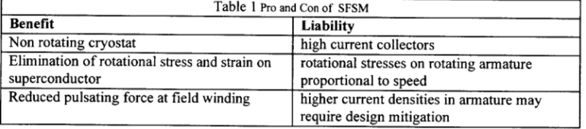
2.1 Pro and Con of the SFSM
The SFSM has been considered on numerous occasions. This topology typically consists of an air-cored superconducting DC field winding (located in the stator), and a rotating armature winding that is normally conducting. The benefits and shortcomings of such a machine have been well treated by Bumby {2}, Mumford
{
1}, and others. These are summarized as follows:Table 1 Pro and Con of SFSM
Benefit Liability
Non rotating cryostat high current collectors
Elimination of rotational stress and strain on rotational stresses on rotating armature superconductor proportional to speed
Reduced pulsating force at field winding higher current densities in armature may require design mitigation
2.2 Motor Topology Selection
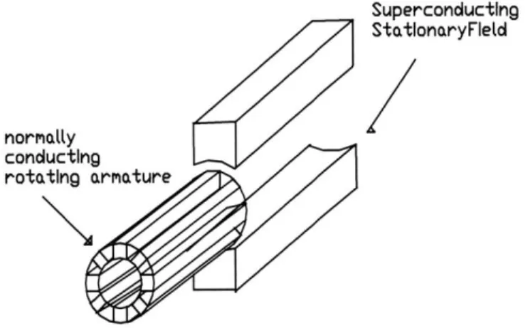
At least two implementations of the SFSM are possible. In the first case, the stationary field is located outside the armature. This implementation is very similar to the usual DC machine.
Mikkonen et al
{
17} have built this version at the Technical University of Munich. A notional schematic is presented in figure 1. below:Superconducting
StationaryFled
normatly
conducting
rotating armature
Figure 1 Type I SFSM Notional Schematic, Field External
Another possible implementation locates the stationary field inside the rotating armature. This implementation seems less conventional. It is depicted below.
Stationary Iron (DC Flux) Rotating Armature
Bearings Torque Tube
Field Winding Support
Cryocoolers Go Here
Thermal Slip Rings
Vacuum Envelope Isolating Supports
Figure 2 Type 2 SFSM Notional Schematic, Field Internal. (taken from SATCON white paper)
The Type 2 SFSM possesses all the favorable characteristics of the Type 1 SFSM. In addition, it also features improved thermal characteristics regarding the superconductor location. Specifically, because the superconductor winding is located inside the armature, it is more concentrated and easier to insulate. Thus, we will consider the Type 2 henceforth.
Rough sizing of the motor is accomplished by utilizing the following equations
T,,otor = 2 -irt -R2 -L --r
where t is the motor shear, defined as: tr = Ba Ko
Of course, from torque the power arises according to:
P = T,,otor * Co
(1)
(2)
(3)
For the notional machine, we select:
" as the motor power, PmOto, a value typical of warship main engines, 30,000 horsepower. " as the motor speed, o, another typical value of 100 revolutions per minute.
* as the motor armature surface current density, K, we select 100000 Amperes/m, on the basis of assumed current density J of 1,000,000 Amperes per square meter applied to a conductor with thickness 0.1 meters.
* as motor length, L, we select 2.5 meters
In addition, we investigate values of Average field flux intensity, B0,
the results detailed in the following plot:.
0 15 10.681, 10 V machine(B o) 5 L2.136.1 0 ' ) LbJ 2 B 0 B,Teslas 4
from 1 to 5 Teslas, with
6
..5.j
Figure 3 Machine Active Region Volume as a function of machine Field Strength needed to produce 30,000 Hp
I I
Note that a typical realistic average flux density for practical superconducting devices is about 2 Teslas at the active region of the armature. For this level of magnetic field, we have a motor volume of about 5 cubic meters, with an associate power density of about 12.5
megawatts per cubic meter'. This agrees well with the theoretical values presented by Tanaka
{6}
2.4 The Nature of Harmonics within the SFSM
It is well known that harmonics of both time and space are ubiquitous to rotating electrical machinery. These harmonics manifest themselves to some degree as a departure from the ideal in characteristics of the machine including terminal voltage and current, and spatial flux distribution. According to Kingsley et al {7}, these harmonics are usually considered to be: harmonics due to non-ideal nature of the windings, harmonics due to the distortion of the magneto-motive force (MMF), harmonics due to saturation of the permeable core material, and harmonics due to the presence of slots and teeth in the construction of the iron in the machine. In a typical synchronous machine, all of these factors must be carefully considered in order to obtain an accurate picture of the machine capabilities. In the case of the SFSM, it is necessary to examine the validity of these concepts as they pertain to the particular case.
2.4.1 Core Saturation Harmonics
Since this SFSM is an air core machine, there can be no saturation of any magnetic material in the core2
. Therefore, this potential source of harmonics may be discounted wholly, at least for this specific class of machine. If the core contains magnetic material, this harmonic source must be considered further.
2.4.2 Slot Saturation Harmonics
' The Active length of the winding is 2.5 Meters, with an overall radius of 1.9 meters
2 There is, however, a magnetic flux shield. This shield is constructed of a magnetic material that can saturate.
Similarly, because the SFSM has no slots (or teeth) in its windings, there can similarly be no harmonics due to these features. It follows that only MMF harmonics and voltage harmonics should be considered in this analysis.
2.4.3 Time Harmonics
Voltage harmonics are usually discussed within the context of machine operation as a
generator, but they are equally meaningful when considering a machine that is motoring since a generated voltage still exists within a motoring machine. This voltage is commonly known as a 'back voltage'. In addition, voltage harmonics might also originate in the motor drive circuitry. Careful design of static inverters and related devices can help insure that voltage harmonics of this origin are minimized. If the design of these devices is not performed carefully, these voltage harmonics can be a significant contributor to noise. These harmonics affect the SFSM just as they would affect a more conventional machine.
For the purposes of this investigation, voltage harmonics will be considered. This is accomplished by assuming a terminal current distortion waveform and modeling this distorted current as a Fourier series.
2.4.4 Space Harmonics
The existence of magnetic field harmonics in the SFSM is also assured simply because the field consists of discrete poles. These will also contribute to the total noise of the SFSM. Indeed, these harmonics might be similar to the harmonics exhibited in any other 3-phase AC rotating electrical machine. Essentially, these harmonics amount to a addition to the field flux by the armature flux, and it is well known that this effect can be quantified by modeling the resulting magnetic field as the Fourier Series representation. This model of the magnetic field may then be used in a force analysis of the standard machine, as is found in Amy
{8}.
In theHowever, it will be assumed that the contributions of the field winding harmonics in excess of the fundamental will not contribute to the acoustic signature due to shell radiation. This is the case because the entire field is stationary in relation to the shell. The field fundamental is so large, however, that the interaction between it and the armature harmonics is significant. Accordingly, the field fundamental will be included in the analysis.
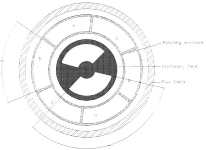
2.5 Machine Topology and Field Modeling
The SFSM of interest is very similar to other superconducting motors, at least from a magnetic field point of view. A significant amount of work has already been done regarding magnetic field modeling in similar machines. The approach has been to model the machine as length independent (ignoring end effects), and then set up the well known scalar magnetic potential problem in two dimensions. This immediately gives rise to the so-called two-dimensional Laplace Equation, which is then solved using separation of variables. For the purposes of this magnetic field analysis, the following figure details the cross section of
interest.
Figure 4 Physical Configuration of the Type 2 SFSM Some of the relevant features are:
* stationary super-conducting field, 2 field poles, of a rather arbitrary 120 electrical degrees each
* rotating armature, 3 armature phases, of 60 electrical degrees " electromagnetic shield of ferromagnetic material
2.6 Force Analysis
Forces within the machine are the source of the acoustic signature we seek to quantify. These forces consist of electromagnetic, aerodynamic, mechanical imbalance, and numerous other mechanical forces. In general, good mechanical design will mitigate all the sources of force
except for the electromagnetic force. This electromagnetic force is also much greater in magnitude than any other force in the machine, for it is precisely this force that is the purpose
of the electric machine.
The electromagnetic force arises directly from the magnetic field intensity within the machine, in a manner fully derived in the following sections. This magnetic field intensity, or H, may be considered to consist of a linear combination of magnetic field contributions due to the superconducting current flowing in the motor field windings, the current flowing in the motor armature windings, and to the time harmonics of the supplied motor terminal current due to the motor power supplies. These components may be superposed since they all exist in a linear medium (air). Once these field components are known, and described
mathematically, they need only to combined to form an aggregate magnetic field intensity. This composite magnetic field is then used to compute forces within the motor.
2.6.1 Magnetic Field Intensity Due to the Superconducting Motor Field Windings
In order to solve the characterize the magnetic field intensity in a generalized electromagnetic problem, the use of the magnetic potential approach is ubiquitous. Depending upon the presence, or absence, of currents, either the scalar or the vector potential is used. Depending upon the existence of currents in the region of interest, either the scalar or the vector
magnetic potential is used. In the case that currents are present in the region of interest, the magnetic field intensity is expressed as a function of a scalar potential such that :
H = -V(D (4) where the scalar potential (I satisfies the Laplace Equation:
V2@ = 0 (5)
which has certain general solutions according to the boundary conditions involved.
In the case of regions in which current is present, it is necessary to express the magnetic field intensity as the curl of vector potential such that:
1(6
H =-(Vx') (6)
where the vector potential 'P satisfies the Vector Poisson Equation:
V2T = -,-, -J (7)
which also has certain solutions according to the particular boundary conditions involved.
In general, both types of regions and their solution methodologies exist in an electrical machine, so that solutions to both the Laplace and the Poisson equations are necessary for a practical electrical machine. In the case of the SFSM, distinct regions exist in the areas of the field winding, the region separating the field from the armature, the armature winding, the region separating the armature from the shield, and in the shield, to name a few. Thus, in order to characterize the magnetic field intensity, it is necessary to expend considerable effort.
Fortunately, Kirtley
{
11}
has solved this problem for a generalized superconducting machine. His results are used in lieu of rigorous solution of these numerous partial differential equations described above.When the applicable Laplace/Poisson Equation for the magnetic scalar/vector potential is solved, as is performed by Kirtley (11
},
the expression for the radial component of the magnetic field intensity due to the field winding is obtained.2-Jf-sin n-- -sinln-p-( - o) n-p+2 -2-n-p
Hi=-2 -r- -p 1 - y.+[ 1 + r (8)
n -(2 + n-p) _ r G R s
2-J f-sin n---f -sin[n.p-(O - I A)] f ) n p+2 - 2.
p-H rf= -H n-t-(2 + 2 )-r. n-p) _ R r -. -p R (8+ )
R s _
n
2.6.2 Magnetic Field Intensity Due to the Motor Armature Windings Similarly, the expression for the armature winding magnetic field intensity is:
Swae)
-sin(n-p0) n-p+22H ra=Y- 2) n. f2 R ao n-p+2) -1 + -r (9)
Hra n.it.(2 + n-p)
_ r JRL s )
_
2.6.3 Magnetic Field Due to Terminal Current Power Supply Time Harmonics
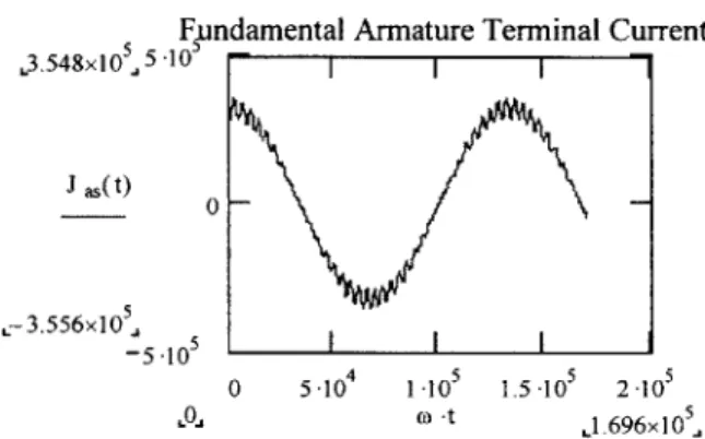
Of course, no power supply employing power electronics is completely free of distortion. Since it is quite likely that this motor will be supplied from a Pulse Width Modulated power supply, the SFSM might need to endure a fairly poor supply power quality.
With this in mind, it is convenient to model the supplied current as a harmonic series.
In this case, the supplied current is that of phase a, with the other two phases being identical save for the phase shift of 120 degrees.
Now this current can be converted to a current density using only the area of the conductor of interest, so that:
Ja(t) = cos(os-t) + (2I - Cos(M-n7))
jImax-sin(opwmt)
(10) where Ac is the area of the armature conductor. This expression for the current density of theOf course, the above is modulated by the appropriate sinusoid if considered as a complete alternating current to the motor.
A graphical representation of notional distorted current waveform as supplied to the motor is presented in the following figure:
0
-3.556x10A
-5-105 ..01
Fpndamental Armature Terminal Current 1An
0 5-104 1-105 1.5-105 2-105
(0 -t L.696x10 5
Figure 5. SFSM Terminal Current
3.548x10⁵J 5
J as(t)
I I I
I I I
2.6.4 The Composite Magnetic Field Intensity
In order to ascertain electromagnetic forces within the motor, it is necessary to obtain an expression for the entire magnetic field intensity in the region of interest (the motor shell). This is accomplished by superposition of the stator magnetic field and the rotor magnetic field. This addition is valid since we are examining said fields in free space, which is a magnetically linear medium. Taking the sum of both the stator and the rotor field, we arrive at the following expression for the composite magnetic field intensity:
Hrtot(t) = Hra(O = o-t) + Hr = (0t) (1
with Hra a function of the armature current density defined above. Now, substituting in for the left-hand terms, we have:
F
(Owmae1
- 2 -J a-s in n 0- ae -s in (n -p -o -t) R ao ) n g + 2 - ) 2
p-H rtot(t) = -
J
.r. n-p+ - xnp+2).L + ( . ..E - n-np(2 + n-p) r R
+ wae + iCn-2
2.J asin n- -sinn-p* O-t + - n.p+2 -2]
+- __ 2 _3 -(R- R n +- + r ... (12)
n.7r. (2 + n-p) r R
0 wae 7 c-23
2-J a-sin n- (3 -sin n-p CO-t 2) ---n.p+2.( . .~p
+ r- Ra -- Xn-p+2)[ 2 r .. n -7.(2 + n -p) _ r R 2 -J -sin n - -f sin [ n -p -((o -t -)] R o ne p+ 2 . ) 2 -n -p +- -)- -- r- (R- yn-p+2).[, + (-r n-7c-(2 + n-p) r RS
Which is the explicit expression for the composite magnetic field intensity in the region of interest for the purposes of obtaining the electromagnetic force produced.
2.6.5 Magnetic Field of Interest in Motor Shell Deflections
In this case, we are only interested in the deflections of the motor shell. This shell is
comprised of a flux shield made of permeable iron, and of various interconnected structural elements between that shell and the motor end bells. Because this shell is stationary, and the motor field winding is also stationary, there will be no time varying nature of the motor magnetic field as experienced by the motor shell. Therefore, all of the terms in the composite magnetic field intensity expression derived in 2.6.4 will not be relevant in determining the electromagnetic force on the motor shell by the time varying fields (as experienced by the
shell). In such a case, only the interaction of the motor field fundamental and the armature harmonics up to arbitrary order, need be considered.
These magnetic fields are calculated and are detailed by the following figure:
Harmonic Fields to Shell in the SFSM 7.04x0J4 8 10 6-104 H ri(t) E H r3( t) 4-10 H r5(t) H r7( t) S -- 2-10 -H r(t) 0 -J- / L-I.316x10 -2-10 0 100 200 300 400 500 1.0 t .450,
Figure 6. SFSM Magnetic Field Intensities
In the above figure, it is interesting to note that the graph is taken from an arbitrary point on the stator, wherein all harmonic fields except the fundamental are time varying with regard to that point of reference. However, the fundamental is stationary from that frame of reference,
In the above figure, it is interesting to note that the graph is taken from an arbitrary point on the stator, wherein all harmonic fields except the fundamental are time varying with regard to that point of reference. Since the fundamental is stationary from that frame of reference, it would appear constant if graphed.
2.6.6 Force on the Motor Shell
The electromagnetic forces that act upon the motor outer shell may now be described. These forces are forthcoming from application of the Maxwell Stress Tensor approach to
calculating forces from magnetic fields. The following section, adapted from Kirtley (3} and Amy {9}, provides the pertinent details of this kind of analysis. The reader is referred to those references for a more detailed derivation.
2.6.6.1 Development of the Maxwell Stress Tensor Approach The Maxwell Stress Tensor is given in Einstein Notation as:
T j=H - S(2 po- - (13)
The force provided by such a distribution is:
{F
-rdv= T i-n dA (14)where Fi is the component of the force density in the ith direction, Tij is the component of the stress tensor in the ith direction on the closed surface normal to the
j
axis, H. and B, are the magnetic field intensity and magnetic flux density in the nth direction, 68 is the kroenecker delta function, and nj is the unit normal in the jth direction.But since length (z) dependence has been neglected, and since we are only interested in the forces on the shell due to the radial magnetic fields, only the T,, term is relevant, and that expression becomes:
Ti = - o H r- H r (16)
and the integral for force defined above becomes:
~ ~~J'~~~ Tind{ !J Firv0 HrHrdA
(17)
fF ;-r dv = fT ij-n jdA = P HrHrdA (7
the question now is, "what is this dA?" In this case, it is the cylindrical coordinates differential area of the cylindrical shell, rdedz, but that is not what is relevant here with respect to the force deforming the shell of the motor. This is the case since the radial component of the motor traction points in the different directions as a function of angular position theta.
A more relevant concept here is the hoop stress, for it is the component of the
electromagnetic stress that tends to deflect the motor shell. Considering this hoop stress the force becomes:
fhOO= M- H,2cos(E)-RdO
(18)
This is a nice expression, except it is deceptively difficult. Recall the H, is an expression involving infinite series. Thus, the force density is an equation that requires integrating an integrand that is a squared infinite series. Clearly, this can be difficult.
2.6.6.2 Simplification of the Force Integral Integrand
In general, the square of a general infinite series (with n taking only odd values)is given as:
I2fn = fn n =f12+2-ff+f3 2
+2-fI-f5+2-f3-f5+ fnI f (19)
n n n n n= 5 ;n=5
(where n assumes all odd integer values)
This is the crux of how we get a tractable integrand in the above force integral.
In the case of the SFSM, the fundamental magnetic field intensity term is the source of the uniform torque in the machine. The higher order harmonics of the total field intensity represent the transient forces in the machine. In the case of the SFSM, the first order (or fundamental) field is largely stationary, so the associated force is not of interest in acoustic analysis. however, the interactions between this fundamental and the higher order harmonics yields steady forces. Additionally, the harmonic field terms squared also represent non-steady forces. These are the terms that must be investigated.
2.6.7 Forces of Interest
As has been discussed, not all of the harmonic terms of the magnetic fields are relevant to the determination of electromagnetic forces on the motor shell in the radial direction. For
example, the motor field fundamental is stationary with regard to the motor shell, and must not be included. This fact is accounted for rigorously by not including the first term of the series squaring operation, which is to say the so-called (f)2 term above. Specifically, this
means the large fundamental term, known as H, is not squared and included in the above force expression integrand .
This is not to say that the fundamental is to be totally discounted, however. It is important to remember that the field fundamental, even though stationary, can still interact with the non-stationary harmonics. This effect is accounted for by the terms that consist of products between the field fundamental and the higher harmonic fields, such as HIH3, HH5 and HH7.
to the shell. These product terms representing the interaction of the fundamental and higher harmonics are likely to contain the largest forces since their constituent parts are much larger than the squaring of the higher order harmonic fields.
2.6.7.1 Forces Arising from Harmonic to Fundamental Interactions
Using the assumed sizing information of section 2.0, the force equations developed above provide numerical values of the forces associated with the interactions between the
fundamental field and the third, fifth, seventh, and ninth harmonics are calculated. The following figure depicts the time varying forces from the first few field harmonic to fundamental interactions: 3.022x10 00 2000 f 13( t) f 1 5(t) f 1 7(t) f 19(t) 0 -2000 -3.0]7x10j -4000 -0 Lo.,
fundamental -harmonic forces
100 200 300 400
Figure 7 Fundamental-Harmonic Forces, per phase
The following table relates the peak amplitudes of these forces: e S Z 021 I' I'. Is' I I I I I I \r
i~7~
J
~ ~ lIp ~ *l~ I ~ / I I I / I I U -' I *dI~ 1,11 XIII III, 500 ,450..Table 2. Harmonic to Fundamental Force Density Amplitudes
Fundamental to Force Density Harmonic #: Amplitude (Pa)
3
5 2333
7 1303
9 715
2.6.8 Conclusions Regarding Forces on the SFSM Stator
So far as the SFSM is concerned, it seems clear that the radial components of forces on the field due to the stator (armature) are very small in comparison to the tip forces (on the rotor) in the motor. This is very significant because it is not the usual case in a synchronous
machine. Specifically, this seems to be because the magnitude of the magnetic field due to the armature is much smaller than the magnetic field due to a field winding (usually placed on the rotor). This is particularly well illustrated by comparing the SFSM pulsating forces with those of a conventional synchronous machine. In fact, the first harmonic force of the SFSM is much less than one percent of the first harmonic force in the conventional machine. This is because, the large magnetic field is kept stationary with respect to the stator of the electrical machine. It seems clear that significant reductions in harmonic forces can be realized simply by adopting the SFSM topology.
Chapter Three. Motor Shell Structural Analysis
3.0 Development of the Acoustic Model
The complete acoustic model necessary for this machine involves multiple sound paths to the far field. The first possible path is direct conduction of sound from the machine to the
propulsor. The second path is direct sound conduction from the machine to the hull via the machine mounting. The third path is sound radiation from the machine shell to the
atmosphere. These distinct paths require different approaches with respect to modeling. All present unique challenges.
Quantification of the first sound path requires modeling the SFSM structure, the structure of the propulsion shaft, and the structure of the propulsor. The nature of the machine and the propulsion shaft are well known, and can be examined rigorously. However, the nature of the propulsor is a more sensitive matter, and cannot be treated in an unclassified manner. In
addition, it is of little utility to model only some of the elements of a sound conduction path, since no useful result is obtained. Thus, this sound path is not examined further.
The second sound path, via the machine acoustic mounting, is also problematic from an analysis standpoint. This is the case since acoustic isolation mounting of machinery is also an extremely sensitive subject with regard to national security. It is fortuitous that limited
unclassified information exists in this area. Due to recent advances in acoustic mounting, it is postulated that this conduction path may be neglected in the very near future. Accordingly, this sound path is not treated in this work.
The third sound path, radiation from the motor shell, is amenable to analysis in this forum. It is essentially the problem of a periodic force acting on a thin cylindrical shell. This force interaction with the shell causes periodic displacements of the shell, with commensurate velocities and accelerations. These velocities and accelerations define the sound transduction of the shell. In principle, this analysis is straightforward mechanics and is generally not classified.
Once the sound is created by the vibrating motor shell, it is carried by the interior medium within the ship. This medium is usually air. This sound traveling in the interior of the ship may be directly perceptible from far field outside the ship. On the other hand, this sound may be received by the hull of the ship, and then radiated to the far field outside the ship. Both cases are generally significant.
3.1 Structural Characterization of the Motor Shell
In order to characterize the acoustic nature of the motor shell, general properties of the shell structure must be discovered. These include the natural frequencies and the mode shapes of the shell. Once these natural frequencies are known for the mode shapes of interest, the proximity of the motor's operating frequencies to these natural frequencies can be determined.
In the event that the natural frequencies are coincident with the motor operating frequencies, there may be resonant behavior of the motor shell. This resonance results in an amplification-like effect on the motor acoustic signature. Such a condition requires a dynamic analysis of the motor shell. This is an analysis based upon solution of the governing partial differential equations of the motor structure. These partial differential equations will contain forcing functions of the form of the motor harmonic forces. In other words, the forcing function is of the form of an infinite harmonic series. In general, solutions of these types of equations are difficult at best, and not always even possible. Because of the adverse effects of resonance on acoustic signature, and the accompanying difficulties of modeling such a physical situation, this condition is to be avoided.
In the event that the resonant frequencies of the shell are sufficiently distant from the operating frequencies of the motor, this resonance is effectively avoided. In this event, In order to obtain an acoustic model of the SFSM, several steps are necessary. First, it is necessary to model the structure of the machine in order to quantify how the pulsating forces
Second, the accelerations thus developed can be utilized as the input to the so-called transfer function analysis (TFA) in order to obtain a sound level. This sound level may then be
compared to the sound levels of other motors in order to quantify the acoustic behavior of the SFSM in some crude way. It should be noted that these analyses are approximate due to the very simplified models of the motor structure, and the first-order estimate nature of TFA. In any case, this method will provide some numbers for the sake of comparison.
3.1.1 Motor Shell Resonant Frequencies and Modes
The determination of natural frequencies and mode shapes of arbitrary physical objects is a topic of ongoing research. Fortunately, for relatively simple geometries, such as finite length cylinders, several references exist that present succinct formulae addressing this problem. Blevins
{16}
presents exhaustive results for all manner of physical geometries, including cylinders of many varied types.3.1.1.1 Details of Thin Shell Equations
Many assumptions are generally made regarding shells in order to characterize them dynamically. For a general cylinder, the following assumptions are common:
" Constant shell thickness
* Shell thickness less than 10% of shell radius
* Linear, elastic, isotropic, and homogeneous material " under no loads
" small deformations in comparison to the shell radius * plane sections remain plane
* rotary inertia and shear are neglected
Beyond these, there are a number of authors who have treated the problem. Authors such as Flugge, Sanders, Mushtari, Donnel, and Reisner are cited by Blevins
{16}..
According to Blevins (16}, the Donnel and Mushtari shell theories are considered simplest, and the Flugge and Sanders theories are considered most accurate. In any event, the problem is generally castas an eighth order differential equation, and differing numbers of terms in the Taylor Series Expansion solution method are retained by the different authors. Blevins
{16}
relates that these eighth order differential equations describe the motion of the shell, and the inertial terms describing the three orthogonal displacement axes are retained for the analysis. Once the spatial dependence of the deformations can be estimated, then the natural frequencies of the shell are forthcoming from the roots of the resulting cubic characteristic polynomial.Blevins
{16}
relates that the analysis of shells is much more complicated than that of plates and beams for many reasons, chiefly because the generality of the shell equations permit a vast variety of mode shapes with accompanying natural frequencies. It is also true that the curvature of shells facilitates a coupling of the extensional and flexural modes of the shell.Such a coupling is not nearly so prevalent in beams and especially plates.
To this end, all formulas for mode shapes and natural frequency generally contain allowances for different and distinct circumferential and axial waves, or modes. These two phenomenon are denoted by a the subscripts i and
j,
respectively. In this way, general expressions for all possible mode shapes are obtained.3.1.1.2 Modes and Resonant Frequencies of the Motor Shell
For the purposes of this analysis, only particular modes and their related natural frequencies will be considered. This is the case because of several reasons.
Since only the radial component of the motor electromagnetic force has been considered, such a component can only excite modes of a radial or coupled radial-axial nature. Such modes are portrayed in the following figure:
Figure 8 Example Shell Mode Shapes For Analysis
These radial only modes are modeled by setting the circumferential mode number i to zero and varying the mode index
j
over integer values to obtain the different radial mode shapes. In the case of the shell modes, Blevins{
16} presents results based upon Flugge Shell Theory. In particular, the Sharma/Johns approximation of Flugge theory is recommended. In this theory, a non-dimensional shell radius to length parameter is defined according to:R S
L (20)
where
j
is the number of the axial mode.A thickness to radius parameter is then defined in accordance with:
ts2
k = 2 1~)
(12-RC
where i is the number of the circumferential mode, set to zero for purely radial modes.
From these definitions, an expression for the non-dimensional frequency parameter is obtained:
X 1 14 + k-i2.P 2[p '2.j2 + 2.v.i2. (2 - i , + 2-(1 - V).(i2 - 1)
2
.a 2] + k-i4. (i2 _ 1)2]
-a 2 + I2(2 +
II
Where the c parameters are taken from Blevins (16}.
Finally, the natural frequency (in Hertz) is obtained:
f i(i) = .ii) )
.
E 2)(2-i-R e _ -( -V I2
(23)
3.1.2 Avoidance of Resonance
The following table relates the natural frequencies of the shell of the SFSM:
Table 3. Shell Radial Mode Natural Frequencies
Mode Number i j=1 j=2
j=3
2 33.06 64.25 94.78
3 21.14 49.17 80.08
4 13.31 34.15 60.68
5 8.97 23.79 44.29
The natural frequencies of the radial shell modes are quite low. The important question is just how close they are to the frequencies of excitation forces due to the electromagnetic
phenomenon of the motor. The following table relates the first several harmonic frequencies associated with these excitation forces:
Table 4. Harmonic Excitation Force Frequencies Force Harmonic Frequency (Hz)
Number 1 120 3 360 5 600 7 840 9 1080
As is evident, the frequencies of excitation of the shell are very much larger than the resonant frequencies of the motor shell radial modes. It is therefore reasonable to assume that
resonance in the radial shell modes is avoided. Because resonance is avoided, the problem can be simplified to a matter of static deflections. This is a much simpler proposition than solving the dynamic equations.
3.2 Shell Deflections Via Static Approach
The solution of the static problem of shell deflection under load is also well treated in the literature. Young (15} provides closed form solutions to the static shell deflection problem for a variety of boundary conditions. These solutions are obtained under the following assumptions:
" the shell of analysis is not under any axial loading
" the magnitude of the deflections are small in comparison to the shell thickness
Neither of these assumptions is overly restrictive for the motor shell under consideration. In the case of the motor shell, it is likely not enduring an axial load since there is in all
likelihood an installed thrust bearing. Furthermore, the shell is constructed of some sort of ferromagnetic steel/iron alloy of considerable thickness, and thus has a sufficiently high modulus of elasticity to ensure that deflections are small in comparison to that appreciable shell thickness.
The solution to the static problem is sensitive to the nature of the force loading on the shell. In general, the electromagnetic force from the motor is not experienced as a point force, but is instead a distributed force that is exerted over some finite area of the shell as the
electromagnetic fields interact. This case is not amenable to the solutions presented by Young {15
},
since no loading case is presented that can account for this arbitrary distributed force. However, from a heuristic standpoint, a concentrated circumferential force of the same magnitude and direction as the sum of the distributed force over the entire force exertion area will deflect a shell more than a that distributed force simply because the force is moreforce per unit length acting on the midpoint of the motor shell interior, as is illustrated in the following figure:
I~4~
Figure 9. Schematic of Static Force Model First define a non-dimensional frequency parameter such that:
(24)
([ V ),+-> .2 5
R S + - -t2
_2) _j
Next, define a thickness parameter:
t3 D =
E-112-(1 - v2] (25)
Now define a family of parameters that are hyperbolic functions of X, shell length, and distance from the force application point to the ends of the shell. These parameters follow:
Ca4 = cosh[(I - a)-k]-sin[( - a)-X] - sinh[(I - a)- X]-cos[(I - a)-X]
Ca3 = sinh[( - a).X]-sin[(l - a)-X)
Ca2= cosh[( - a).X]-sin[(1 - a)-k] + sinh[(I - a)-X]-cos[(1 - a)-X]
Cal = cosh[( - a)-.X].cos[(l - a)-X]
C14 = (sinh(1.x)) 2 + (sin(I-?))2 C13 = cosh(I-X).sinh(1-X) - cos(I-X)-sin(I-x) C12 = cosh(1.X)-sinh(1.X) + cos(I.X).sin(.x) C1I = (sinh(1.X))2 - (sin(I.k))2 (26) C4 = cosh(-x)-sin(1.X) - sinh(I-X)-cos(I-X) C3 = sinh(-X)-sin(1-X) C2 = cosh(1.X)-sin(1-X) + sinh(1.X)-cos(I-X) C1 = cosh(1-X)-cos(-1))
Now define the shell flexural angles at end A and B of the shell:
( Q (C2-Ca2 - 2.C3-Cal)
~Va =2Dx2 I
2-D-k2 Cli
(27) Wb = Va'Cl - Ya'C4-k - PCa3
2-D-X
Now define the deflection equations at each end of the shell as a function of these parameters: ( -Q 3 (C3-Ca2 - C4-Cal) 2-D-k3 Cli (28) Yb = YaCi + Wa- -2F- -2.)L 4-D-k
From these equations, numerical values of deflection for each harmonic force component are calculated. The following table relates these deflections:
Table 5. Shell Deflections from Force Harmonics Force Harmonic Number Deflection (meters)
End A End B
1-3 0 0
1-5 -7.84E-06 1.25E-07
1-7 -4.38E-06 6.97E-08
1-9 -2.40E-06 3.82E-08
The deflections are quite small, as is to be expected. The differences in sign from end to end arise as a result of the coupling between circumferential and axial strain within the curved shell geometry.
3.3 Shell Vibration Velocities
In order to obtain an acoustic signature, it is necessary to convert these displacements to velocities, commonly known as vibration velocities. This can be accomplished by dividing each deflection by its period. These velocities are presented in the following table:
Table 6. Shell Vibrational Velocities
Force Harmonic Number Velocity (meters/second)
End A End B
1-3 0 0
1-5 -4.70E-03 7.49E-05
1-7 -3.68E-03 5.85E-05
1-9 -2.60E-03 4.13E-05
These velocities represent the deflections at the ends of an open cylinder. The deflections of an enclosed cylinder will be smaller due to the restrictive nature of the rigid ends. The
differences from end to end is due to the mode shapes of the curved shell. These mode shapes arise from the complex coupling relationships of the circumferential and axial strain.
3.4 Sound Radiation from the Shell
The details of sound transduction from the shell can be approached in a number of ways. Methods ranging from Hamiltonian Mechanics found in Belman {14} to elementary transfer function analysis presented by Amy {9} are found in the literature. These two approaches illustrate the extremes in complexity and detail. Belmans { 13} presents finite element method solutions to very complex models
3.4.1 Ideal Sound Radiator Theory
A commonly used method for sound wave generation modeling is the construct of the sound radiator. This methodology has been applied to electrical machinery by P.L. Timar, et al in
{ 13 }. In this work, the sound radiator approach is utilized. Essentially, this approach uses the propagation characteristics of known simple geometries (such as point sources, plane
sources, cylinders, and spheres) in order to approximate the sound propagation of real and more complicated geometries. According to TIMAR, the use of either cylindrical or spherical sources approximate the sound radiation characteristics of real electrical machines quite well. Both the cylindrical and the spherical radiator have been used to model electric machines as acoustic sources. While it heuristically appears that the cylindrical radiator should more accurately model a cylinder-like machine, it turns out that the end effects of the finite machine shell cause a departure from ideal cylindrical behavior, and a spherical model is more accurate.
3.4.2 Spherical Radiator Equations
In accordance with Timar, the development of the general theory of geometric sound radiators is as follows.
For an arbitrary sound wave, the wave number k is defined as:
k=2- (
Where the A is the wavelength of the sound, defined as:
C
f (30)
The pressure deviation due to the spherical sound wave is given as:
p = al eJ(O vibetkr) (31)
The velocity of the same spherical sound wave can be described by:
= P al j(o
v=- . re
viet-kr) P aJ.ei ( vie-t-k-r+ )
vbt- r)+ P -] e2 (k-r )
The associated sonic impedance is the defined as:
= V (33)
Substituting (33) and (34) into (35), we obtain:
Z = p-c-k-r-FF (k.r)
1
1
I + k2 r _ 1 + k. r 2)j
(34)
From this acoustic impedance, the acoustic radiated power is given as: P=Re{Z}-S-v2 (35)
Taking the real part of (36) and substituting into (37) gives: p -c -k2 r )-SV2 (36)
1+k2
r2
Finally, the sound power level provides a metric of the radiated noise level, and is defined as: L, = 20 -log - (37)
Where PO is a reference power level, taken to be 1 mW (10-3 W)
Chapter Four. Acoustic Modeling
4.0 Development of the Acoustic Spectrum of the SFSM
In order to obtain a meaningful results of the radiated sound power level from the SFSM, it is necessary to combine the results of chapter three. Specifically, the vibration velocities
obtained from the structural analysis will be combined with the acoustic radiator modeling. This procedure is straightforward.
4.1 Combining the Vibration Velocities and the Acoustic Analysis to Obtain a Theoretical Acoustic Signature
Taking the velocity results from Table 7 and substituting these into (38) and (39) provides numerical values of the acoustic power level from the SFSM. This acoustic power level, as stated previously, is a result relative to a reference power level of one milli-Watt. The following table relates these results:
Table 7. Radiated SFSM Shell Acoustic Power Level Motor Harmonic Numbers Acoustic Power Level
dB (rel. to ImilliW ref.)
1-3 N/A
1-5 52.8
1-7 48.6
1-9 42.5
4.2 Acoustics Signature of the SFSM Shell
SFSM Shell Acoustic Power Level E 60.00 0o 40.00 20.00 -0.00 (I> 3 5 7 9
Harmonic Interacting with the Fundamental
Figure 10. SFSM Radiated Acoustic Power
It is interesting to note that the largest sound level in the is about 64 dB Although Acoustic source levels are not well reported in the literature, anecdotal evidence from Amy {9}, Timar (13 }, and Belmans { 14} indicates that peak sound power levels in other types of motors are
much higher than those of the SFSM. It is further important to note that the above 'spectrum' really only constitutes about one octave of interest in the acoustic spectrum. This octave is, however, the one including the greatest sound power levels of any octave. This analysis does not address the other octaves. In any case, this is quite a significant difference for the octave
Chapter Five. Comparison of SFSM to Conventional
Machine
5.0 Acoustic Comparison of SFSM with a Conventional AC Superconducting Motor The crux of the problem is just how much quieter a machine with a stationary field winding will be as compared to a machine with a rotating field winding. It has been proposed by
Timar
{
13} that fixing the largest magnetic field in an electrical machine will make the machine quieter. This section seeks to quantify this heuristic assertion.5.1 Conventional Machine Description
For the purposes of comparison, a rotating field superconducting machine of the same ratings and physical dimensions is postulated. The existence of similar environmental shielding, current densities, and other basic physical parameters is also assumed.
5.2 Forces of Interest In the Conventional Machine
For reasonably similar machine topologies with the same number of phases, any two machines of a given power rating will have similar electromagnetic forces .This is the case because it really makes little difference whether the field is stationary or moving with respect to the armature. In fact, these forces will also have similar harmonic components, as well. Ostensibly, this seems to suggest that the machines will radiate the same amount of noise. It is true that, for most machines, noise is largely a function of power rating.
In the case of different motors, this is not the whole story. The salient aspect here is which of the forces is able to excite a sound radiator and do so efficiently. In the case of the SFSM, it has been demonstrated that the fundamental component of the machine electromagnetic force is stationary in time and space, and therefore cannot excite any acoustic transduction in any of the motor components and subassemblies that are also stationary. Since the largest surface areas of an object form the largest radiated acoustic power signals from that object, the fact that the shell is not excited by the fundamental means that a large amount of radiated noise is