Spreadsheet based teaching aids
in chemical engineering education
Georges Heyen , Boris Kalitventzeff
Laboratoire d'Analyse et Synthèse des Systèmes Chimiques, Université de Liège, Sart Tilman building B6, B-4000 Liège (Belgium)
phone +32 4 3663521, fax +32 4 3663525, email G.Heyen@ulg.ac.be
Abstract : Modern spreadsheet programs offer a wide range of calculation, charting and dialog options, allowing
the development of effective teaching aids. Examples of worksheet illustrating numerical analysis, thermodynamics and unit operations are shown. All offer complete interaction between the problem statement and the presentation of results.
Keywords : Teaching, interactive calculation, spreadsheet. INTRODUCTION
Everyone seems to use spreadsheets these days. This type of software tool has become one of the most popular personal computer activities, second only to word processing, both in frequency of use and variety of applications.
Relatively few people however are aware of the extensive mathematical problem solving capabilities that have been built into modern spreadsheet programs : equation solving, curve fitting, statistical analysis, optimization are the most convenient ones. Combining these rich mathematical features with extensive charting tools, and with the capability to build easily elaborate user interfaces, modern spreadsheet packages can also be used as teaching aids, to illustrate some important concepts in a vivid way.
This paper aim is to present some applications we have developed at Université de Liège. We expect to make them available to the chemical engineering community through EURECHA, the European Committee for Computers in Chemical Engineering Education (see http://www.capec.kt.dtu.dk/eurecha/). By doing so, we hope to foster the development of many more such educational applications.
WHY TO USE INTERACTIVE TEACHING AIDS
New concepts are only mastered when they are put into practice. Ideally, any theoretical development exposed during a lecture should be reviewed in an application. However many concepts involve a range of variables, whose interactions are not always easy to grasp. Solving a single example is not enough to illustrate most of the possible combinations. Analyzing an algorithm for some extreme conditions is also instructive (e.g. Newton's method when the Jacobian matrix is close to singular, or a distillation design when reflux gets close to minimum).
We favour learning by doing. We think that numerical experimentation, made easy with a convenient user interface, allows to gain better, faster and deeper
understanding.
Present personal computers now have the power to solve many simple engineering problems in real time. Spreadsheet programs also provide facilities to combine calculations, data tables, text, graphs and versatile dialog items (scrollbars, buttons, counters, list box, etc) that allow the students to interact with the concepts they have to understand.
SOME TYPICAL EXAMPLES
Some examples are described her below, to illustrate our approach. The first two illustrate numerical methods (optimization). The next two show the behaviour of popular physical property models : a cubic equation of state and an activity coefficient model. The last two are based on unit operations : distillation and stirred tank chemical reactor with heat exchange.
Optimization : the Nelder-Mead algorithm
The simplex algorithm proposed by Nelder and Mead (see Himmelblau 1972) is very robust optimization method, suitable for problem involving a small number of variables. The spreadsheet illustrates the behaviour of the algorithm for a few typical objective functions, selectable using a list box. Figure 1 illustrates the optimization of Rosenbrock function :
f(x,y)=Ln[100(y-x2)2+(1-x)2]
The "Initialize" button generates a simplex around the initial point. The variables and objective function values are displayed in the table below. The simplex also appears on the graph.
By pressing the "Iteration" button, one step of the simplex algorithm is carried out. The worst point of the simplex is reflected through the centroid of all other points, and if this step is successful, an expansion is attempted. Alternatively, a contraction or a reduction of the simplex may be carried out to allow the simplex to "take a turn" or to "sink in the valley". The "Optimize" button let the program iterate until the optimum solution is found within the prescribed tolerance. The user can visualize the simplex crawling
on the graph, and changing shape in order to adjust itself to the local pattern of the objective function.
Optimization: Levenberg-Marquardt method
The goal of this example is to visualize and compare the gradient and Newton's direction for different local features of an objective function. Here again, the Rosenbrock function is taken as an example.
The user can move a pointer on the 3D chart using a horizontal and a vertical scrollbar. Numerical values
are updated in the attached table : independent variables, function value, gradient and hessian matrix. The eigenvalues of this matrix are also displayed. The quadratic approximation to the objective function is also illustrated : its contour line passing through the base point is shown. The user can verify it is an ellips when the eigenvalues are positive, and a hyperbola when they differ in sign, which is the case for the example shown.
The gradient direction and Newton's step are shown on the chart. The user can visualize how these directions are oriented according to the location on the map. In the present case, the Newton's direction points toward a saddle point, and it may not always correspond to a descend direction.
When one eigenvalue is negative, an optimization step can be calculated by the Levenberg-Marquardt algorithm (Himmelblau 1972), by adding a positive constant to the diagonal elements of the hessian matrix. A scrollbar allows to adjust this constant, and view how the algorithm works. The contour line of the modified approximation (forced to be elliptical) and the modified step are also shown on the graph.
Thermodynamics : A Cubic equation of state
The example shown is based on the Soave equation (Soave 1972) .The goal is to demonstrate to the student how the pure component parameters (critical temperature and pressure Tc, Pc, acentric factor ω) allow to calculate the equation of state parameters. All intermediate numerical values are displayed. An isotherm is drawn as P vs log(V) for a selected temperature. When this temperature is modified using the scroll bar control, the graph is updated in real time, which makes it very easy to show the difference between subcritical and supercritical isotherms. A horizontal bar corresponding to a selected pressure also appears on the graph, and the selected pressure can also be modified using a scroll bar control. The equation of state expressed in cubic form for the given T and P is displayed on the second chart. This shows that the equation may have either one or three Figure 1 : Optimization with a flexible polyhedron search
Nelder -Mead : illustration
2 variables Epsilon= 0.0001 Objective Variables function x1 x2 3.639 -0.97960 1.54311 min -2.70000 1.30000 max -0.20000 1.80000 number 41 41
Tolerance Iteration Evaluation
Simplex 0.6297 5 10 x Reflection x1 x2 - 3.639 -0.97960 1.54311 + 2.398 -1.16458 1.60561 4.076 -1.43131 1.32121 o -1.29794 1.46341 r 3.639 -0.97960 1.54311 2.398 -1.16458 1.60561 Iteration Optimize 3D plot Initialise Rosenbrock(log) 8.00-9.00 7.00-8.00 6.00-7.00 5.00-6.00 4.00-5.00 3.00-4.00 2.00-3.00 1.00-2.00 0.00-1.00 -2.7 -2.2 -1.7 -1.2 -0.7 -0.2 0.3 0.8 1.3 1.8 -0.2 0.2 0.6 1.0 1.4 Figure 2 :
Newton and Levenberg-Marquardt algorithms
x y Variables 0.360 1.010 Function f = 39.165 = m (y-x^2)^2 + (1-x)^2 m = 50 Gradient -64.669 = - 4 m x(y-x^2) -2 (1-x) 88.040 = 2m (y-x^2) Hessian -122.24 -72.00 2-4m(y-3x^2) -4 m x -72.00 100.00 -4 m x 2 m eigenvalues 121.287 -143.527 -0.0074 -0.8857 is a descent direction β 200.94 140 H + I β 78.70 -72.00 -72.00 300.94 Step 0.7093 -0.1228 Next x,y 1.069 0.887 3.0-4.0 2.0-3.0 1.0-2.0 0.0-1.0 -1.0-0.0
real roots, according to the values of T and P. The solution(s) of the equation of state can also be sought numerically using Newton's method. Initial values of the compressibility factor Z have to be set in the appropriate cells (0 is recommended for ZL and 1
for ZV). The values corrected by performing a
Newton's step are displayed in the adjacent cells. The iteration values are displayed as small dots on both charts. Next iteration can be carried out by pressing the lower button on the sheet ("Next Z iteration"). Liquid and vapour fugacity coefficients φL and φV are
also calculated. When convergence on both ZL and
ZV is achieved, they should coincide if the pressure is
the saturation pressure at the fixed temperature. Otherwise, a better estimate of the pressure is :
P P L
V
* = φ
φ .
The pressure is updated according to this scheme when the middle button is activated ("Next Pvap iteration"). The complete iterative calculation leading to the vapour pressure evaluation is carried out until convergence when the top button is pressed ("Calculate Pvap").
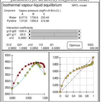
Thermodynamics : binary coefficients in NRTL model
This examples allows to illustrate the form taken by VLE phase diagrams, and how the dew and bubble point curves are affected by modification of the binary coefficients in the NRTL model (Renon 1969). Four sets of experimental data are provided, corresponding to typical diagrams : quasi ideal mixture, positive or negative deviation, formation of two liquid phases.
The user may change the values of the 3 binary coefficients using scrollbar controls. The phase diagram and the y vs x diagram are updated in real time. A least squares objective function is also evaluated, form the departures between the experimental and predicted vapour compositions and bubble pressures.
Finding the optimum by trial and error is not obvious, due to significant interaction between the parameters : similar diagrams can be obtained with quite different parameter values. When the user estimates the best parameters has been obtained, the numerical optimizer can be activated to achieve the very best; watching the optimizer performing also provides clues on how an optimization algorithm proceeds.
Reaction engineering : multiple steady states in a C.S.T.R. thermal balance.
This example illustrates the occurrence of multiple steady states for a jacketed stirred tank reactor where an exothermal reaction takes place.
The volumes of the reactor and the jacket must be fixed, as well as the product of exchange area by the heat transfer coefficient. Reaction data (first order rate constant, activation energy and heat of reaction) must be initialized. The reactant flow rate, the inlet concentration and temperature must be given. These data fix the reactor characteristics (the sigmoid curve showing the difference between energy released by the reaction and energy transported by convective flow).
The coolant flowrate and inlet temperature can then be manipulated using scroll bars, which move the line
Figure 4 :Vapour-liquid equilibrium, fitting parameters for an activity coefficient model
Isothermal vapour-liquid equilibrium NRTL model Vapour pressure (logPv=A-B/(t+C) )
A B C Water 8.0713 1730.6 233.43 Pyridine 7.0133 1356.9 212.66 Interaction coefficients g12-g22 1320.0 116 50 20 g21-g11 -20.0 99 100 20 a12 0.2850 57 0 0.005 G12 G21 a12 t12 t21 SSQ 0.5850 1.0082 0.2850 1.8809 -0.0285 Optimize 933.08
Figure 3 : a cubic equation of state
Soave equation of state Vapour pressure calculation P=R T/(v-b) - a(T)/(V(V+b)) Component data Propane T 321.0 K A c Tc 369.82 K P 16.673 bar B d Pc 42.496 bar e ω 0.1454 (-) R 0.0831 m3 bar/K Tr Z f(Z) df/dZ New Z ! " a(Tc) 9.5095 Pr Liquid # # b 0.0627 a(Tr) # Vapor # # # # #
k(ω) 0.7051 a(T) $ % $ & & & 16.6741 bar P new = P guessed * PhiL/PhiV
' &$ ' ( % $ &$ $ ) )$ ( % $
Figure 5 : multiple steady states in a CSTR
Reactor thermal balance
0 1000 2000 3000 4000 5000 6000 0.0 20.0 40.0 60.0 80.0 100.0 120.0 Gen.-conv. Heat exch.
corresponding to the coolant energy balance. For some values of the coolant rate and temperature, three steady states can be identified.
To go on with the analysis of the reactor operation, a full dynamic simulation model can then be used to model either the start up of the reactor or a change of operating conditions.
This spreadsheet can be used in parallel with the Control Station software (Cooper 1998), which provides a simulation of the same reactor with several control schemes (manual control, PID control of the reactor product composition by adjusting the coolant flow rate, cascade control).
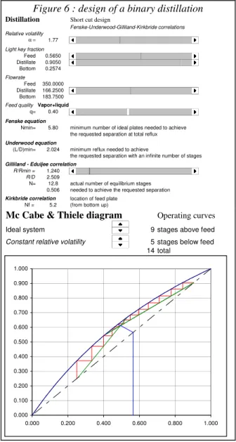
Unit operations : Binary distillation
This spreadsheet allows to analyze ideal binary distillation, and to explore the key variables that affect distillation column performance.
A first worksheet allows to perform a short-cut design of a binary distillation column, using a series of well known correlations (Fenske Underwood Gilliland -Kirkbride, e.g. see Kister 1992).
First the relative volatility α has to be adjusted using a scrollbar control. The light component molar fraction in the feed and in the distillate are also
specified in the same way, as well as the distillate flow rate and the feed thermal state.
The bottom flow rate and composition are automatically computed from the mass balance. A warning message flags unfeasible specifications. Minimum number of trays and minimum reflux are estimated using Fenske and Underwood equations. When the user specifies the reflux ratio, the actual number of equilibrium stages and feed tray location are also calculated from Gilliland and Kirkbride correlations.
The operating conditions can be visualized on a McCabe and Thiele diagram, whose main features are automatically adjusted from the same control as for the design calculation. The user is also allowed to modify the number of equilibrium stages using stepper controls. The operating diagram is continuously updated, which makes it easy to visualize the occurrence of pinch points or the effect of reflux ratio on the column performance.
BENEFITS
The benefit of using interactive tools to demonstrate technical concept lies in the possibility to show a large number of examples with a single spreadsheet. Usually, various features can be explored by varying a single parameter at a time.
A recommended approach is to start with a straighforward example, where, for instance, a numerical method works very efficiently, and later to show pitfalls, or limits of the method by selecting ill-conditioned cases.
Our experience is that students better grasp new concept when they can see how they are applied. They even understand better when they can use demo materials by themselves, and experiment at their own pace.
CONCLUSIONS
Spreadsheet programs available now offer a powerful and low-cost capability to develop interactive demonstration of technical concepts.
We propose to collect similar examples and to distribute them to the educational community through the EURECHA channel.
REFERENCES
Gottfried B. S., Spreadsheet Tools for Engineers. McGraw-Hill (1996)
Himmelblau D.M., Applied Nonlinear Programming., McGraw-Hill (1972)
Renon H., J.M. Prausnitz, AIChE J., 15:785 (1969) Soave G., Chem. Eng. Sci. 27:1197 (1972)
Cooper D.J., Control station User Guide, http://www.eng2.uconn.edu/control/ (1998) Kister H.Z., Distillation Design, McGraw-Hill (1992) EURECHA web site :
http://www.capec.kt.dtu.dk/eurecha/ Figure 6 : design of a binary distillation
Distillation Short cut design
Fenske-Underwood-Gilliland-Kirkbride correlations Relative volatility
α = 1.77 77
Light key fraction
Feed 0.5650 113 Distillate 0.9050 181 Bottom 0.2574 0.257 Flowrate Feed 350.0000 Distillate 166.2500 95 Bottom 183.7500
Feed quality Vapor+liquid
q= 0.40 18
Fenske equation
Nmin= 5.80 minimum number of ideal plates needed to achieve the requested separation at total reflux Underwood equation
(L/D)min= 2.024 minimum reflux needed to achieve
the requested separation with an infinite number of stages Gilliland - Eduljee correlation
R/Rmin = 1.240 24 R/D 2.509
N= 12.8 actual number of equilibrium stages 0.506 needed to achieve the requested separation Kirkbride correlation location of feed plate
Nf = 5.2 (from bottom up)
Mc Cabe & Thiele diagram Operating curves
Ideal system 9 stages above feed
Constant relative volatility 5 stages below feed 14 total 0.000 0.100 0.200 0.300 0.400 0.500 0.600 0.700 0.800 0.900 1.000 0.000 0.200 0.400 0.600 0.800 1.000