High Level Power Estimation for DSP

HAL Id: hal-00077587

https://hal.archives-ouvertes.fr/hal-00077587

HAL is a multi-disciplinary open access

archive for the deposit and dissemination of sci-entific research documents, whether they are pub-lished or not. The documents may come from teaching and research institutions in France or abroad, or from public or private research centers.

L’archive ouverte pluridisciplinaire HAL, est destinée au dépôt et à la diffusion de documents scientifiques de niveau recherche, publiés ou non, émanant des établissements d’enseignement et de recherche français ou étrangers, des laboratoires publics ou privés.

High Level Power Estimation for DSP

Johann Laurent, Nathalie Julien, Eric Martin

To cite this version:

Johann Laurent, Nathalie Julien, Eric Martin. High Level Power Estimation for DSP. 2000, pp 112-117. �hal-00077587�

Abstract :

We present here a high level power estimation method for Digital Signal Processor (DSP) based on an original functional analysis together with practical validations. Instead of classical methods conducted at instruction level, we evaluate the power consumption of a whole algorithm at a behavioural level; first are extracted for the given algorithm characteristics such as parallelism rate, cache miss rate, memory mode... and then these parameters are applied to empirical consumption laws. As example, the energy model elaborated for a TEXAS INSTRUMENTS DSP is provided; our method applied to classical algorithm (FIR ) has also been validated by measurements.

1.

Introduction

Power optimisation is currently recognised as a major issue for future developments in telecommunication applications in order to reduce both the weight and the size of the batteries, to increase the autonomy of portable applications or to moderate the cooling system.

To be power efficient, algorithm transformations in addition to technological optimisations are essential [1]; furthermore, such modifications are easy to applied and allow to decrease the time-to-market. However, to evaluate the power impact of these transformations, we need to estimate the application consumption at the early stage of the system design.

In 'process greedy' applications such as the new information and communication technologies, the use of the last DSP generation has been largely extended in order to improve the computation possibilities. These processors are characterised by complex architectures: a deep pipeline, VLIW control instructions, memory caches and possibly superscalar architectures. Moreover, it is well-known that the power consumption part due to the external memory access is a more and more

important problem in this kind of applications [1-4] ; so the power estimation model has to take into account this aspect. Even if there are some advanced works on memory optimisation, they are poorly related to an estimation method able to predict the power consumption of a whole algorithm [5].

Differing of all the other recent works on power consumption optimisation for DSP [2], we have chosen to conduct the study at a behavioural level instead of the instruction level in order to avoid two main problems: on one hand, a "low level" approach does not consider the other architectural components such as memory and on the other hand, being at a behavioural level allows to include optimisations through compiler directives and high level code transformations.

Furthermore, at this time, the only way proposed to evaluate power consumption at the instruction level implies, for a given DSP, to first measure all the different instructions set and their interactions [2,3]. So even when the DSP is slightly modified (as a new version of the same architecture), all the measures have to be achieved again; in addition, with the last DSP generation, the available instructions are so numerous that the characterisation measurements are very time expensive.

Section 2 will present the framework of the methodology and its implementation to a specific DSP, the TEXAS INSTRUMENT TMS320C6201. Afterwards, section 3 develops the power characterisation for the main functional blocks and the empirical consumption laws that we have obtained. Finally, in section 4 we present the application of our method on one typical processing algorithm (a FIR) and the validations of these results with measurements.

2.

Methodology and functional analysis

A. Framework of the methodology

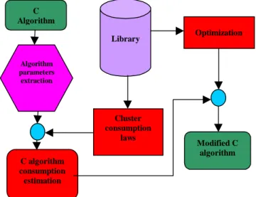
Our purpose is to develop power optimisation strategies on DSP programming for an algorithm in C language as represented in Figure 1.

SAME 2000

Session 6: EDA/FLOW

High Level Power Estimation for DSP

Johann LAURENT, LESTER Laboratory

Nathalie JULIEN, LESTER Laboratory

Eric MARTIN, LESTER Laboratory

To validate the efficiency of different optimisation techniques, it is convenient to be able to predict the power consumption of the initial algorithm and its modifications through a complete estimation method. To prove the reliability of the estimates, the definition of a precise measurement methodology is also needed. These measures must be executed rapidly and have to characterise accurately the DSP power behaviour in relation with the task it has to execute.

First, from the C algorithm are extracted different parameters characterising this algorithm and the different functional clusters it uses: the clock frequency F, the execution time Texe, the memory mode, if necessary the cache miss rate, the parallelism rate for the processing units, the number of memory access... Then, we use a toolbox called Cluster consumption laws to estimate the power consumption of each functional cluster used by the algorithm and, by combining these estimates, to evaluate the power consumption of the whole algorithm. The next toolbox Optimisation is used for rewriting the C algorithm.

Figure 1 Complete methodology of power estimation and reduction

To construct the toolboxes Cluster consumption laws and Optimisation, we must realise a complete library which encloses empirical but accurate power consumption estimates validated by measurements.

The new DSP generation can have an elaborated architecture since it can integrate a deep pipeline, VLIW control instructions, internal memories that can be used in cache mode and parallelism possibilities for the instructions. On the hardware point of view, each different architectural component contributes to the entire power consumption of the processor. But current compilers optimise very efficiently the parallelism both for the instructions and for the processing. The only part that is not properly treated by the compilers is concerning the memory management (cache memory, external access…). So the designers are concentrating

all their efforts on this problem and there is a strong need of adapted estimation and optimisation tools. B. General functional analysis

For realising the library, we use a functional analysis based on a power consumption study of the DSP architecture including its pipeline. All the functional blocks are analysed, developed and reorganised in clusters which are architectural components defined according to their impact on energy dissipation and their interactions. The general representation presented in Figure 2 can be modified for a particular DSP, by adding or/and removing some clusters.

After analysis, we obtain four different functional blocks: MMU (Memory Management Unit), IMU (Instructions Management Unit), PU (Processing Unit), CU (Control Unit). In a second time, we determine the interactions between the different clusters and we qualify them in terms of power consumption.

MMU: Management Memory Unit CU: Control Unit

IMU: Instructions Management Unit PU: Processing Unit

Figure 2: Functional analysis example

From this analysis we define three steps for determining the power consumption of a block. First all the characteristic parameters of the block are described i.e. for the program memory part, the cache miss rate, the memory mode… as illustrated later. Then, a set of testing programs called scenarios are developed: either we can determine one scenario that includes only a block (or a cluster) or this power part is defined relatively to the others by varying the scenario. Then, time and current measurements (absolute or relative) are performed leading to the energy. This approach allows us to obtain finally direct relations between architecture and power consumption.

C Algorithm Algorithm parameters extraction C algorithm consumption estimation Cluster consumption laws Library Optimization Modified C algorithm DMA MMU CTRL registers Peripheral bus PLL Interruptions CU FETCH stages CTRL/MEM PRG IMU REGISTERS UAL / MPY DECODE stages CTRL/MEM DATA PU

C. Specific functional analysis on Texas Instruments TMS320C6201

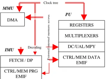
This last generation processor uses a complex architecture with a deep pipeline (up to 11 stages), VLIW instructions, parallelism possibilities (up to 8 parallel instructions) and its internal program memory can be used in cache mode. In Figure 3, the result of this specific functional analysis is presented with only interactions between blocks for more clearness.

This DSP has a particular block which is the External Memory InterFace (EMIF), used for all the external memory access and then appearing for both the program memory (IMU) and the data memory (PU). It also contains two different registers files and multiplexers that allow to cross the datapath and represented as new clusters. Moreover, it could be noticed that the DECODE stage of the pipeline is now separated into two steps: the dispatching part (DP) of the instructions is included in the IMU and only the instruction decoding (DC) is remaining in the PU.

Figure 3: Interactions for the TMS320C6201 The interactions between the CU and all other clusters through the control registers are negligible because these registers are rarely modified during the algorithm execution. Another weak link is the one between the DMA (Direct Memory Access) and the fetch stages (IMU) because, for the mapped memory mode, the DMA can only be used to load the internal program memory at the boot phase. On the other hand, an important interaction exists between the MMU and the PU through the loading of data from an external memory via the DMA. We also have a relation between IMU where instructions are loaded and the PU where they are executed. Otherwise, the Clock Tree is a strong interaction for all the clusters. Indeed, for the new DSP generation, this frequency can be up to 300MHz and the clock tree consumption can represent up to 40% of the global energy.

The characterisation of these blocks, clusters and their interactions by consumption laws is presented below.

3.

Power characterisation of functional

blocks and clusters

Two kind of measures has to be realised, one for measuring the average current dissipated by the DSP core Icore and another to obtain the execution time of the program Texe. The energy per iteration E can also be determined by knowing these two parameters and the core supply voltage Vdd (2.5V) via the expression (1):

E = Icore * Texe * Vdd (1)

The scenarios (testing programs) are actually written in assembler in order to excite each cluster individually; they are composed of an unbounded loop which size ensures that its effect to the dissipation is negligible relative to all the rest of the scenario. With the different measures obtained by varying each parameter for a given block or cluster, we can determine the evolution of the power consumption.

We will present as example in the next section, the achieved work on the IMU block containing the fetch stages and the program memory.

A. The FETCH/DP cluster

As the TMS320C6201 processor uses VLIW instructions and therefore loads several instructions in the same time, the consumption of the fetch stages can not be neglected. The power consumption of this cluster depends on two parameters: the frequency F and the parallelism rate α. When α=1, both the parallelism and the fetch excitation are maximum and 8 instructions are loaded at each cycle to be executed in parallel. When α=1/8, the excitation is minimum and so 8 instructions are loaded all the 8 cycle times because the instructions will be executed sequentially. By analysing the assembler source, it is easy to deduct the average parallelism rate for the whole algorithm or a part of it.

On the Figure 4, the results confirm that the current is linear with the frequency and increases with the parallelism rate. It has to be noticed that is represented the current used by the fetch stages IFETCH together with the clock tree current ICLK and the current of the internal program memory IPRG. FETCH / DP CTRL/MEM PRG EMIF IMU DMA MMU REGISTERS MULTIPLEXERS DC/UAL/MPY CTRL/MEM DATA EMIF PU Ex te rn a l/in te rn a l memor y a ccess Decoding Clock tree

Figure 4: Current variations for the FETCH/DP cluster

From these measures, we establish a consumption law given by the expression (2):

ICLK+FETCH+PRG = (aα + b) F + cα + d (2)

ICLK+FETCH+PRG : average current (mA)

F : frequency (MHz) a = 5.21mA/MHz; b = 4.19mA/MHz c = 42.4mA; d = 7.6mA α parallelism rate 1/8 1/5 1/2 1 E µjoule/iteration 100 98 77 27

Figure 5: Energy variations for the FETCH/DP cluster

Finally, we remark that the energy per iteration E is constant in the frequency domain for a given parallelism rate α as represented in Figure 5. It corroborates that the energy is optimised when the parallelism rate increases, that can be completely managed by the compiler.

B. Memory modes

If we consider now the second cluster of the IMU block, it concerns the program memory part. The first parameter that we can define for this cluster is the memory mode of the algorithm (or part of it) which has an important effect on the final power consumption.

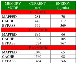
So we will present here the results obtained for the four different modes of the internal program memory. For the MAPPED mode, all the program is in the internal memory. In the CACHE mode, external accesses are done when the instructions are not in the cache (case of a cache miss). The FREEZE mode is similar to the CACHE mode except that the cache is only read and never written. For the BYPASS mode, all the instructions are read in the external memory.

MEMORY MODE CURRENT (mA) ENERGY (µjoule) F = 40MHz MAPPED 281 70 CACHE 448 112 BYPASS 369 369 F = 133MHz MAPPED 886 66 CACHE 1399 105 BYPASS 1224 367 F = 160MHz MAPPED 1040 65 CACHE 1560 98 BYPASS 1464 366

Figure 6: Memory modes characteristics Figure 6 shows the variations of both the average current used by the DSP core and the energy used for a iteration of the program. As the scenario generates no cache miss, the results for the FREEZE mode are similar to those for the CACHE mode.

First, we can confirm that the current is not a sufficient parameter. Indeed, the BYPASS mode absorbs less current than the CACHE mode (about –16%) but it consumes more energy (about +250%) without considering the additional energy cost of the external memory and I/O buffers.

The energy for each memory mode is also stable with the frequency. Of course, the most efficient mode is the MAPPED one. We can characterise the others relatively to it with about +35% of energy cost for the cache management and around +400% for the BYPASS mode.

C. Memory cache

The other parameter concerning the program memory cluster in the case of the memory cache mode is the cache miss rate γ. As explained before, the complexity of the embedded applications is ever-increasing with the needs of memory space. As the internal memory size is limited, the use of external memory is often necessary to the good execution and it is better for the programmer to use the CACHE mode. But once the cache is used, it implies that cache misses may appear together with supplementary consumption due to the external accesses and due to the I/O buffers.

We have done measures to know how the energy evolves with the cache miss rate.

In Figures 7 and 8, are represented the execution time Texe and the measured average energy per iteration E for the same scenario as functions of the cache miss rate γ in percentage for F=160MHz and α = 1.

0 50 100 150 200 250 300 350 400 0 50 100

CACHE MISS RATE (%)

EXECUTION TIME (µs)

Figure 7: Execution time versus γ We can remark that the execution time Texe can be written relatively to N, the number of cycles for the execution of the program and the frequency F by the expression (3)

Texe = N (n,α,γ)/F (3)

and N can also be defined as a function of the number of the instructions in the program n, α and γ. Each time a cache miss appears, the pipeline is frozen and then the number of cycles increases rapidly and the energy follows this rising.

Figure 8: Cache miss energy versus γ Finally, for this example, we can see that there is an over-consumption of more than 2000% between a program with no cache miss and a program with γ = 100%. It could be noticed that this energy also varies with the parallelism rate α but these variations are less predominant; for γ = 0%, the energy dissipated for α=1 is 300% lower than for α=1/8 and this gap shrinks about –15% at γ =100%. In conclusion, it is more important to avoid the cache misses before improving the parallelism rate.

Such a similar method has been used to determine the laws for the other blocks and clusters of the functional analysis.

In this section, we present a method used to estimate a whole algorithm (for the moment at assembler level). We will use a typical signal processing algorithm: a FIR filter. We will compare the result of our estimations with measures for validating our method.

A. Estimation method

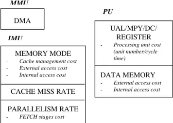
The estimation method is based on the functional analysis that we have presented above. We use also the consumption laws that we have determined for each functional block. Figure 9 represents the different parameters to take into account for the architecture presented as example.

Figure 9: Estimation functional parameters Generic parameters of the algorithm are the frequency F, the execution time Texe, the number of instructions n, the number of cycles N.

For the IMU block, the functional parameters that we have to extract are: the memory mode, if the CACHE mode is operating, the cache miss rate γ and the parallelism rate α..

For the PU block, we determine its cost by knowing the average number of used processing units per cycle time β. The consumption law for this cluster (PU) is given in expression (4).

IPU = 0.64βF (4)

β: average number of processing units used per cycle time.

F: Frequency (MHz).

Another parameters concern the data storage with the number of external Mext and internal Mint accesses and the possible use of the DMA.

When all costs of the different blocks are known, the application can evaluated by addition of all the different clusters costs.

DMA MMU

UAL/MPY/DC/ REGISTER - Processing unit cost

(unit number/cycle time)

DATA MEMORY - External access cost

- Internal access cost MEMORY MODE

- Cache management cost

- External access cost

- Internal access cost CACHE MISS RATE PARALLELISM RATE - FETCH stages cost

IMU PU 0 200 400 600 800 1000 1200 1400 1600 0% 50% 100%

CACHE MISS RATE ENERGY by iteration (µjoule) α = 1 0 200 400 600 800 1000 1200 1400 1600 0% 50% 100%

CACHE MISS RATE

ENERGY by iteration

(µjoule)

B. Estimation example

The considered application is a FIR filter that uses 16 coefficients stored with all the samples in internal data memory. First, we must extract the different parameters of this algorithm:

- α = 0.36 - F = 160MHz - γ = 0

- memory mode = MAPPED - β = 1.595

- Texe = 52.5µs

Then, we inject these parameters in the consumption laws that we have shown above. The results are listed below:

ICLK = 4.19F = 670.4mA

IFETCH = 5.21αF+42.401α+7.6 = 323mA IPU = 163mA

The global consumption is the addition of the different consumption:

Σ = ICLK + IFETCH + IPU = 1156.4mA i.e.

151.8µjoule.

Figure 10: Repartition of the energy

Figure 10 show that the main consumption is due to the clock tree (58%), the second consumption is due to the FETCH stages (28%) and the last one is due to the PU (14%).

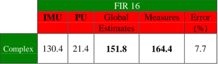
The results are presented in Figure 10 for complex coefficients. FIR 16 IMU PU Global Estimates Measures Error (%) Complex 130.4 21.4 151.8 164.4 7.7

Figure 10: FIR 16 energy estimations and measures (in µjoule per iteration)

The error estimation is less than 8% and actually, we think that this problem is due to the estimation of the PU. Indeed, if a lot of loads are made by the program, so several delay times are generated and thus the average

number of processing units per cycle time become improper. Future works will have to take into account this parameter to improve our consumption model: we could divide the PU block in two parts, one for the load aspect and another for the processing.

One of the next works will also be to validate our method with a more complex application and, if possible, to compare our results with those of an instruction level model.

5.

Conclusion

We have introduced an original high level power estimation method providing the energy estimates of an entire algorithm; this method is conducted through a behavioural analysis of the DSP architecture instead of the usual approach conducted at the instruction level. This technique has been implemented on one of the last generation of TEXAS INSTRUMENTS DSP (TMS320C6201) with a complex architecture. Generic parameters of the considered algorithm are extracted such as the memory mode, the parallelism rate, the cache miss rate… and are applied to empirical consumption laws providing the dissipated current and the energy for each functional part of the circuit. The results obtained for a FIR algorithm, at the assembler level, have been validated by measurements with an error of less than 8%. In future works, after having improved this promising method for other applications, the final purpose of the project will be to extend it to the estimation of C language algorithms.

Acknowlegments:

References

[1] J.M. Rabaey, M. Pedram "Low power design

methodologies" Kluwer Academic Publishers 1996.

[2] Vivek Tiwari, Sharad Malik, Andrew Wolfe "Power

analysis of embedded software: a first step towards software power minimisation." IEEE Transactions on VLSI Systems,

December 1994.

[3] Mike Tien-Chien-Lee, Vivek Tiwari, Sharad Malik and Masahiro Fujita "Power Analysis and Minimisation

Techniques for Embedded DSP Software." IEEE Transactions

on VLSI Systems Vol5 N°1 March 1997.

[4] P. Vanoostende et al. "Issues in low power design for

telecom" IEEE 1995 pp 591-593.

[5] Berkeley Design Technology, inc.

www.bdti.com/articles/lowpower.htm 1994.

[6] M.C Rinard "Compiling for low power consumption"

www.cag.lcs.mit.edu/~~rinard/F98.6.892/handouts/h2/ 58% 28% 14% CLK FETCH PU