HAL Id: hal-00725576
https://hal.archives-ouvertes.fr/hal-00725576
Submitted on 27 Aug 2012
HAL is a multi-disciplinary open access
archive for the deposit and dissemination of
sci-entific research documents, whether they are
pub-lished or not. The documents may come from
teaching and research institutions in France or
abroad, or from public or private research centers.
L’archive ouverte pluridisciplinaire HAL, est
destinée au dépôt et à la diffusion de documents
scientifiques de niveau recherche, publiés ou non,
émanant des établissements d’enseignement et de
recherche français ou étrangers, des laboratoires
publics ou privés.
3D Mesh Skeleton Extraction Using Topological and
Geometrical Analyses
Julien Tierny, Jean-Philippe Vandeborre, Mohamed Daoudi
To cite this version:
Julien Tierny, Jean-Philippe Vandeborre, Mohamed Daoudi. 3D Mesh Skeleton Extraction Using
Topological and Geometrical Analyses. 14th Pacific Conference on Computer Graphics and
Applica-tions (Pacific Graphics 2006), Oct 2006, Tapei, Taiwan. s1poster. �hal-00725576�
3D Mesh Skeleton Extraction Using Topological and Geometrical Analyses
Julien Tierny, Jean-Philippe Vandeborre
∗and Mohamed Daoudi
∗FOX-MIIRE Research Group – LIFL (UMR USTL/CNRS 8022)
∗
GET / INT / T´el´ecom Lille 1, France
{tierny, vandeborre, daoudi}@lifl.fr
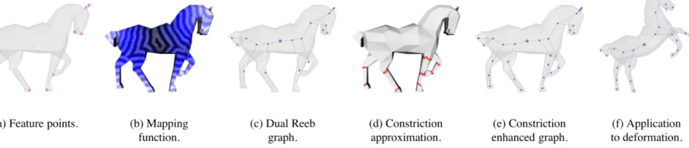
(a) Feature points. (b) Mapping function. (c) Dual Reeb graph. (d) Constriction approximation. (e) Constriction enhanced graph. (f) Application to deformation.
Figure 1. Main steps of presented method on a standard model.
Abstract
This paper describes a novel and unified approach for Reeb graph construction and simplification as well as con-striction approximation on 3D polygonal meshes. The key idea of our algorithm is thatdiscrete contours – curves
car-ried by the edges of the mesh and approximating the con-tinuous contours of a mapping function – encode both topo-logical and geometrical shape characteristics.
Firstly, mesh feature points are computed. Then they are used as geodesic origins for the computation of an invari-ant mapping function that reveals the shape most significinvari-ant features. Secondly, for each vertex in the mesh, itsdiscrete contour is computed. As the set of discrete contours
recov-ers the whole surface, each of them can be analyzed, both to detect topological changes or constrictions. Constriction approximations enable Reeb graphs refinement into more visually meaningful skeletons, that we refer as enhanced topological skeletons.
Without pre-processing stages and without input pa-rameters, our method provides nice-looking and affine-invariant skeletons, with satisfactory execution times. This makes enhanced topological skeletons good candidates for applications needing high level shape representations, such as mesh deformation (experimented in this paper), retrieval, compression, metamorphosis, etc.
1. Introduction
Polygonal mesh is a widely used representation of 3D shapes, mainly for exchange and display purposes. How-ever, many applications in computer graphics need higher level shape descriptions as an input. Topological skeletons have shown to be interesting shape descriptions [2]. They benefit diverse fields like shape metamorphosis, deforma-tion [13], retrieval [10], texture mapping, etc.
Many topological approaches study the properties of real valued functions computed over triangulated surfaces. Most of the time, those functions are provided by the application context, such as scientific data analysis [4]. When deal-ing with topological skeletons, it is necessary to define an invariant and visually interesting mapping function, which remains an open issue [2].
Moreover, traditional topological graph construction al-gorithms assume that all the information brought by the mapping function is pertinent, while in practice, this can lead to large graphs [18, 5], encoding noisy details.
Finally, topological approaches cannot discriminate vi-sually interesting sub-parts of identified connected compo-nents, like the phalanxes of a finger. This is detrimental to certain applications, such as mesh deformation.
In this paper, we propose a novel and unified method which addresses the above issues. Given a connected tri-angulated surfaceT , feature points are firstly extracted (fig. 1(a)) in order to compute an invariant mapping function, notedfm(fig. 1(b)), which reveals the shape most
signifi-cant parts. Secondly, for each vertex in the mesh, we com-pute its discrete contour, a connected curve traversing it and locally minimizingfmgradient. We show that a topological
analysis of those discrete contours enables a pertinent Reeb graph construction and simplification (fig. 1(c)), without any input parameter. Finally, we show that a geometrical analysis of discrete contours can approximate constrictions on prominent components (fig. 1(d)), enabling the refine-ment of Reeb graphs into enhanced topological skeletons (fig. 1(e)).
This paper is structured as follows. Firstly, we introduce topological skeleton related work. Secondly, we define our mapping functionfm. Thirdly, we present our algorithm for
discrete contour computation, which is used both for the Reeb graph construction and simplification as well as the constriction approximation. Finally, we comment on exper-imental results and discuss about possible applications, like mesh deformation (fig. 1(f)).
2. Related work
Several approaches have been explored for the de-composition of polygonal meshes into meaningful sub-components, to extract skeletal representations of shapes.
In comparison to mesh segmentation [20] and traditional skeleton extraction [3, 24], topological approaches, based on Morse and Reeb graph theories [16, 19, 15], present the advantage to preserve the topological properties of the shape [2] (number of loops, number and relations between components, etc.). However, with regard to shape skele-tons, we identify three main drawbacks in topological ap-proaches, successively addressed in this paper.
Firstly, it is difficult to define an invariant and visually interesting mapping function. Secondly, constructing and transforming a topological graph into a manageable skele-ton is not a trivial problem. Finally, topological approaches decompose a surface into connected sub-components only. This means that visually interesting sub-parts of identified connected components will not be discriminated: for exam-ple, a finger of a hand model will not be decomposed into phalanxes.
2.1. Mapping functions
Differential topology based approaches study the proper-ties of real valued functions, that we refer as mapping
func-tions, defined on input surfaces, either to construct Reeb graphs [22, 6], contour trees [5], level set diagrams [12] or Morse complexes [18, 4]. Those functions are often brought by the application context: terrain modeling [22], MRI anal-ysis [5], molecular analanal-ysis [4], etc.
When dealing with topological skeletons, it is necessary to define a scalar function which satisfies invariance and stability constraints, and which also affords a topological
description that highlights visually significant surface sub-components.
Lazarus and Verroust [12] introduced such a function, defined by the geodesic distance (the length of the short-est path between vertices) from a source vertex to any other vertex in the mesh. It leads to visually interesting results for natural objects because it is invariant to geometrical trans-formations and it is robust against variations in model pose [11]. Due to a lack of stability, within the framework of shape retrieval, Hilaga et al. [10] proposed to integrate this function all over the mesh. Unfortunately, from our experi-ence, that function generates an important amount of criti-cal points, configurations where the gradient of the function vanishes, which makes the construction of visually mean-ingful graphs more complex.
In our method, to reveal the shape most significant fea-tures, we focus on feature points. Feature points are mesh vertices located on extremities of prominent components [11]. Mortara and Patan`e [17] proposed to select as fea-ture points the vertices where Gaussian curvafea-ture exceeds a given threshold, but this cannot resolve extraction on con-stant curvature areas. Katz et al. [11] developed an algo-rithm based on multi-dimensional scaling in quadratic exe-cution complexity. In this paper, we propose a robust and straightforward algorithm for feature point extraction (fig. 1(a)). Moreover, we use them as geodesic origins for the definition of our mapping function (fig. 1(b)). Such a func-tion well reveals the most visually significant parts of the mesh, generating manageable critical point sets.
2.2. Graph construction and simplification
A Reeb graph [19] is a topological structure that encodes the connectivity relations of the critical points of a scalar function defined on an input surface. More formally, Reeb graphs are defined as follows:
Definition 1 (Reeb graph) Let f : M → R be a scalar
function defined on a compact manifoldM . The Reeb graph
off is the quotient space of f in M × R by the equivalence
relation(p1, f (p1)) ∼ (p2, f (p2)), if and only if:
f (p1) = f (p2)
p1andp2belong to the same connected
component off−1(f (p 1))
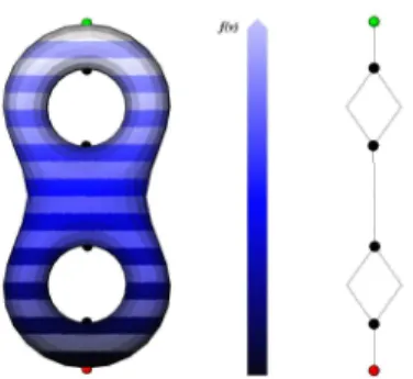
Figure 2 gives an example of a Reeb graph computed on a bi-torus with regard to the height function and well illustrates the fact that Reeb graphs can be used as skeletons. Constructing a Reeb graph from a scalar functionf com-puted on a triangulated surface first requires to identify the set of vertices corresponding to critical points. With this aim, several formulations have been proposed [7, 23] to identify local maxima, minima and saddles, observ-ing for each vertex the evolution off at its direct neigh-bors. Several algorithms have been developed to construct
Figure 2. Evolution of the level lines of the height function on a bi-torus, its critical points and its Reeb graph.
Reeb graphs from the connectivity relations of these critical points [6, 5], most of them in O(n × log(n)) steps, with n the number of vertices in the mesh. However, they as-sume that all the information brought by the scalar function f is relevant [18, 5]. Consequently, they assume that all the identified critical points are meaningful, while in prac-tice, this hypothesis can lead to unmanageably large Reeb graphs. To overcome this issue, Ni et al. [18] developed a user-controlled simplification algorithm. Bremer et al. [4] proposed an interesting critical point cancellation technique based on a persistence threshold. Attene et al. [1] proposed a seducing approach, unifying the graph construction and simplification, but it is conditioned by a slicing parameter.
In this paper, we propose a discrete formulation of con-tours, connected subsets of level lines, which enables, with-out any input parameter, the construction of visually mean-ingful Reeb graphs (fig. 1(c)).
2.3. Constriction computation
H´etroy and Attali [9] define constrictions as simple closed curves, whose length is locally minimal. Con-strictions are located on the narrowest parts of a surface. This notion is of major interest for segmenting individ-ual subcomponents identified with standard topological ap-proaches into more significant parts, for deformation pur-pose for example. Recently, H´etroy [8] showed that con-striction detection could be achieved by analyzing surface curvature.
In this paper, we propose to analyze the geometrical characteristics of discrete contours, and particularly their concavity, to approximate constrictions (fig. 1(d)), in order to decompose previously identified components into more visually interesting parts (fig. 1(e)).
3. Method overview
Given a connected triangulated surface T , we propose in this paper a unified method to decomposeT into visu-ally meaningful sub-parts, considering the topological and geometrical characteristics of discrete contours.
The algorithm proceeds in three stages. Firstly, mesh feature points are extracted (fig. 1(a)) in order to compute an invariant and visually interesting mapping function (fig. 1(b)), denoted fm in the rest of the paper. Secondly, for
each vertex in the mesh, we compute its discrete contour, a curve traversing it and approximatingfmcontinuous
con-tour. Finally, as the set of discrete contours recovers the entire mesh, it is possible to analyze each contour charac-teristics, either to detect topological changes (fig. 1(c)) or to detect curvature transitions (fig. 1(d)).
Our scientific contribution resides in three points. (i) We propose an original and straightforward algorithm for feature point extraction. It can resolve extraction on con-stant curvature areas – such as spheres – and it is robust against variations in mesh sampling and model pose. (ii) We show that a discrete contour formulation enables, with-out re-meshing and withwith-out any input parameter, a perti-nent Reeb graph construction, providing visually meaning-ful graphs, affine-invariant and robust to variations in mesh sampling. (iii) We show that the geometrical information brought by discrete contours enables the approximation of constrictions on prominent components and consequently Reeb graph refinement.
4. Mapping function
To compute visually meaningful topological skeletons, we first have to define a mapping function that will high-light the most significant parts of the mesh. In order to fit application constraints, this function has to present stability and invariance properties. Geodesic distances are affine-invariant and robust to variations in model pose. From an algorithmic point of view, they can be approximated by the Moore-Dijkstra algorithm (distance minimizing in weighted graphs). In the rest of this paper, we will refer to δ(v1, v2) as the normalized approximation of the geodesic
distance from vertexv1to vertexv2, normalized with regard
to mesh global extrema.
4.1. Feature point extraction
Feature points are mesh vertices located on extremities of prominent components. As they highlight the most sig-nificant features of the shape, they are used in our mapping function computation as origins for geodesic distance eval-uation. To extract them, we propose a quite straightforward algorithm, based on topological tools. Most of the geodesic based mapping function local extrema appear at extremities of prominent components (figs. 3(a) and 3(b)), mainly be-cause gradient vanishes in those configurations. Therefore, we propose to realize a crossed analysis, using two geodesic based mapping functions – whose origins are the mesh most distant vertices – and to intersect the sets of their local ex-trema.
(a) E1. (b) E2. (c) E1∩E2.
Figure 3. Feature point extraction overview.
Letvs1 andvs2 be the most geodesic distant vertices of
a connected triangulated surfaceT , computed with the Tree Diameter algorithm [12]. In figure 3, vs1 is located at the
extremity of the wrist (fig. 3(a)) whilevs2 is located at the
extremity of the middle finger (fig. 3(b)).
Letfg1 andfg2 be two scalar functions defined on each
vertexv of T , as follows:
fg1(v) = δ(v, vs1) (1)
fg2(v) = δ(v, vs2) (2)
Basing on the critical point classification proposed in [6], a local minimum is defined as a vertex such that all its direct neighbors have an upper function value. Reciprocally, we define a local maximum as a vertex such that all its direct neighbors have a lower function value. LetE1 be the set
of local extrema (minima and maxima) of fg1 (in yellow
in fig. 3(a)) andE2 be the set of local extrema offg2 (in
cyan in fig. 3(b)). Extremities of prominent components are configurations wherefg1 andfg2 tend to an extremum
(figs. 3(a) and 3(b)). Consequently, the set of feature points is both included inE1andE2. Therefore, we define the set
of feature pointsF of T (fig. 3(c)) as follows:
F = E1∩ E2 (3)
In practice,fg1andfg2 local extrema which correspond
to feature points do not appear exactly on the same vertices but in the same geodesic neighborhood. Therefore, the in-tersection constraint is relaxed as follows, with " ∈ [0, 1] the radius of the geodesic neighborhood (geodesic distance are normalized): v ∈ F ⇐⇒ ∃ve1 ∈ E1 / δ(v, ve1) < " ∃ve2 ∈ E2 / δ(v, ve2) < " δ(v, vfi) > " ∀vfi ∈ F "∈ [0, 1] (4)
From our experience, using only two geodesic mapping functions (fg1 andfg2) and setting " = 0.05 give accurate
results. Moore-Dijkstra’s algorithm is a time complexity bottleneck.fg1andfg2are computed each inO(n×log(n))
steps, withn the number of vertices in T .
In this paragraph, we presented a straightforward algo-rithm for mesh feature point extraction, inO(n × log(n)) steps, withn the number of vertices in T . This algorithm is based on geodesic distance evaluations. Therefore it is sta-ble and invariant to geometrical transformations and robust
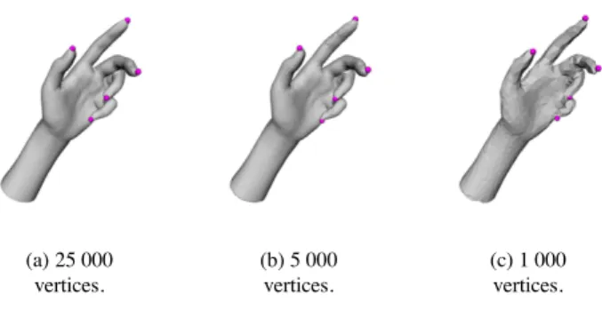
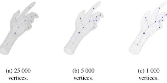
(a) 25 000 vertices. (b) 5 000 vertices. (c) 1 000 vertices.
Figure 4. Feature point extraction robustness against mesh sampling variations.
to variations in model pose. Furthermore, in order to select feature points, the mapping function gradient is analyzed. No hypothesis is required about mesh sampling. Conse-quently, this algorithm is robust against variations in mesh sampling, as illustrated in figure 4: feature points are similar when the resolution decreases. Moreover, it achieves cor-rect extraction on constant curvature areas, such as spheres, as shown in fig. 5(a).
4.2. Mapping function computation
When dealing with topological skeletons, it is necessary to define an invariant and visually interesting mapping func-tion, which reveals the most significant parts of the mesh. Moreover, the mapping function should not generate an un-manageable set of critical points, in order to make the graph simplification easier. From our experience, this is not the case of the function presented in [10].
Firstly, to guarantee invariance to geometrical transfor-mations and robustness against variations in model pose, geodesic distances are used. Secondly, to define a visu-ally interesting mapping function, feature points are taken as origins for geodesic distance evaluations. Therefore, we propose the following mapping function, notedfmin the
rest of the paper, which computes in each vertexv of T the geodesic distance to the closest feature point:
fm(v) =
fc(v) − minv∈Tfc(v)
maxv∈Tfc(v) − minv∈Tfc(v)
(5) fmis a normalized version of the functionfc, defined as
follows (fc(v) ≥ 0, ∀v ∈ T ):
fc(v) = 1 − δ′(v, vc) (6)
withvcthe closest feature point fromv:
vc∈ F / δ′(v, vc) = minvfi∈F δ(v, vfi) (7)
Notice thatfmis invariant to uniform scaling (thanks to
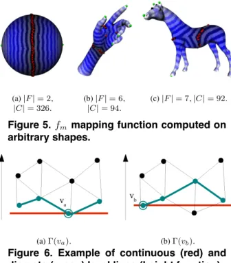
the normalization), rotation and translation (thanks to the use of geodesic distances). Figure 5 presents some compu-tations offmover arbitrary shapes, the number of extracted
feature points (|F |) and the number of critical points (|C|, identified according to the classification proposed in [6]). fmhas been defined so as it tends to maxima (in green) at
(a)|F | = 2, |C| = 326.
(b)|F | = 6, |C| = 94.
(c)|F | = 7, |C| = 92.
Figure 5.fmmapping function computed on
arbitrary shapes.
(a) Γ(va). (b) Γ(vb).
Figure 6. Example of continuous (red) and discrete (green) level lines (height function).
feature points and it tends to minima (in red) at the center of the object.
As shown in figure 5,fm generates an important
num-ber of critical points. Consequently, standard Reeb graph construction algorithms would create large graphs, count-ing as many nodes as critical points, which is a major issue for topological skeleton extraction. In the next section, we present a formulation of discrete contours, which enables a unified graph construction and simplification process.
5. Discrete contours of a mapping function
In this section, we propose to construct discrete
con-tours. In the next sections, those discrete contours will be used either to detect topological changes or to detect curva-ture transitions, providing enhanced topological skeletons, without re-meshing and without any input parameter.
Defining contours of a real function f computed on a triangulated surfaceT is not a simple problem. In the con-tinuous case, two pointsp1andp2belong to the same level
linef−1(f (p1)) if f (p2) − f (p1) = 0. Moreover, p1and
p2 belong to the same contour if they belong to the same
connected component off−1(f (p 1)).
In the discrete case, for a given vertexv ∈ T , depending on T sampling, f−1(f (v)) is often reduced to the vertex
v itself. With regard to definition 1, a correct Reeb graph could not be constructed from this formulation of discrete contours, because the conditions of the equivalence relation would rarely be satisfied.
To preserve contour topological properties in the
dis-(a) Γ(v600), 2 contours. (b) Γ(v10 000), 4 contours. (c) Γ(v20 000), 6 contours.
Figure 7. Example of discrete level lines on a 25 000 vertex mesh (fmfunction).
crete case, we define the discrete level line Γ(v) associ-ated to the vertexv as a curve computed along the edges of T which approximates by upper value the continuous level linef−1(f (v)). Figure 6 shows discrete level lines
travers-ing an arbitrary triangulation, with regard to the height func-tion. Moreover, each connected subset of a discrete level
lineis referred as a discrete contour. In particular, we de-fine the discrete contour γ(v) associated to the vertex v as the connected subset of Γ(v) containing v. Notice that the moreT will be dense, the more discrete contours will tend to continuous contours.
Discrete contourscan be computed for the whole mesh using a step by step gradient ascent process, described in algorithm 1. It handles two heaps, respectively the set of visited verticesV t and the set of candidate vertices for visit Cd. At each step, Cd surrounds V t by upper value.
Algorithm 1 Discrete contour computation.
V t = ∅
Cd ← {argminv′∈Tf (v′)}
whileCd .= ∅ do
v ← argminv′∈Cdf (v′)
5: Γ(v) ← Cd
γ(v) ← connected subset of Cd, containing v Removev from Cd
Cd ← Cd ∪ {v neighbors, which are not in V t} Addv to V t
10: end while
A discrete level line locally minimizes its difference with the continuous level line it approximates. This difference can be expressed as follows:
%
vi∈Γ(v)
(f (vi) − f (v)) / f (vi) ≥ f (v), ∀vi∈ Γ(v) (8)
In expression 8,f (v) is a constant term. Consequently, minimizing this expression is equivalent to minimizing f (vi) which is actually performed at each iteration of
al-gorithm 1. Cd always surrounds V t by upper value and minimizes expression 8, thus it is equivalent to Γ(v).
(a) 1 contour.
(b) 2 contours.
(c) 1 contour.
Figure 8. Bifurcation and junction contexts on a torus shape (height function).
(a) (b) (c)
Figure 9. Dual Reeb graphs of primitive and complex shapes (fmfunction).
shown, at different iterations i of the algorithm. V t ver-tex set is displayed in white and Γ(v) is displayed in red. Visiting in a recursive fashion each vertex of Γ(v) enables the identification of each of its connected subsets, and par-ticularly γ(v).
6. Topological analysis of discrete contours
Standard Reeb graph construction algorithms need sim-plification in order to remove noisy details. In this section, we propose a unified algorithm for graph construction and simplification, based on the topological analysis of discrete contours. Following the definition 1 of a Reeb graph in the continuous case, we can state an analog equivalence rela-tion in the discrete case between two verticesv1, v2 ∈ T ,
based on our notion of discrete contour: (v1, f (v1)) ∼ (v2, f (v2)) ⇐⇒
&
v2∈ Γ(v1)
v2∈ γ(v1) (9)
v1 and v2 belong to the same connected component if
they satisfy the above conditions. Therefore, at each itera-tion of the contour computaitera-tion algorithm, each individual connected component ofT , traversed by Γ(v), can be iden-tified. Thus, topological changes can be detected observing the numberNΓ(v)of connected subset of Γ(v), as f evolves. We define three types of topological changes:
1. bifurcations: whenNΓ(v)increases from iterationt to iterationt + 1 (Γ(v) splits in two contours from 8(a) to 8(b)),
2. junctions: whenNΓ(v)decreases fromt to t + 1 and when several discrete contours merge (two contours merge in one from 8(b) to 8(c)),
(a) 25 000 vertices. (b) 5 000 vertices. (c) 1 000 vertices.
Figure 10. Algorithm robustness against mesh sampling variations.
3. terminations: whenNΓ(v) decreases fromt to t + 1, without discrete contour merge.
Figure 9 shows several dual Reeb graphs obtained with this strategy, with regard tofm. Connected components are
represented by the nodes located at their barycenter. The main contribution of our algorithm is that graph con-struction and simplification are performed at the same time. If we compare figures 9 and 5, we notice that the dual Reeb graphs do not reflect the presence of noisy critical points (points in red in figure 5), because discrete level lines do not disconnect in those configurations. Standard Reeb graph al-gorithms would have generated graphs counting as many nodes as critical points – 94 nodes for the hand model and 92 nodes for the horse model – while in our approach only meaningful topological variations are encoded in the graph. In comparison to [1, 10], no re-meshing and no input parameter, such as a slicing parameter, are required. Con-sequently, as no assumption is made about T sampling, this algorithm is robust against variations in mesh sam-pling, as shown in fig. 10. Furthermore, asfmis based on
normalized geodesic distance evaluations, presented graphs are also invariant to geometrical transformations (rotation, translation and uniform scaling).
In this section, we presented a unified graph construction and simplification algorithm, based on the topological anal-ysis of discrete contours. As contours do not disconnect in fmnoisy parts, resulting graphs reveal the shape most
sig-nificant features. However, a strict topological analysis can-not discriminate visually meaningful sub-parts of a given connected component. To overcome this issue, we propose in the next section to analyze the geometrical characteristics of discrete contours to detect constrictions.
7. Geometrical analysis of discrete contours
Constriction approximations enable the subdivision of the branches of topological skeletons into more visually in-teresting parts. In this section, we propose an algorithm for constriction approximation, based on the analysis of the curvature of discrete contours. For each discrete contour identified in the previous stage, we compute its Gaussian curvature and we identify local minima as constrictions.
Model fτ = 3 fτ= 5 fτ= 10 fτ = 15 Humanoid 4 8 9 12 Horse 1 11 11 11 12 Hand 1 5 8 11 12 Hand 2 6 9 11 11 Horse 2 9 14 19 19
Table 1. Number of constrictions with differ-ent concavity curve cutoff frequencies (fτ).
7.1. Topological constraint
Since constrictions are defined as closed curves, the anal-ysis has to be restricted on closed discrete contours only. Considering each contour γ(v) as a connected and non-directed planar graphG, γ(v) is a cycle, and consequently a closed curve, if the degree of all its vertices equals two. Therefore for each discrete contour ofT reduced to a pla-nar graphG, the degree of each of its vertex is computed and we only consider in the rest of our algorithms contours that satisfy the above property.
7.2. Concavity curves
In our experiments, the average curvature ζ(γ(v)) of each discrete contour γ(v) is estimated by computing the Discrete Gaussian Curvature [14] in each of its vertex. If ζ(γ(v)) is positive, γ(v) neighborhood is globally convex, otherwise it is concave. Constrictions appear on the narrow-est, or the most concave, parts of a surface. Consequently, in order to only consider concave discrete contours, we com-pute ζ′ (γ(v)) as follows: ζ′ (γ(v)) = & ζ(γ(v)) if ζ(γ(v)) ≤ 0 0 if ζ(γ(v)) > 0 (10) During the discrete contour computation, each contour is stored in the related node of the dual Reeb graph. As this algorithm visitsT from the lowest to the highest fmvalues,
for a given node of the graph, contours are automatically sorted byfmvalues. Computing ζ′(γ(v)) sequentially for
each of these sorted contours gives, for a given node, a
con-cavity curve, an overview of the concavity evolution asfm
evolves.
Curves shown in figure 11 give examples of such evolu-tions, computed on the neck of the horse model (fig. 12(j)). The left values of these concavity curves correspond to the concavity estimations of the discrete contours located at the basis of the neck. The right values correspond to the con-cavity estimations of the discrete contours located at the end of the neck (basis of the head sub-part).
7.3. Constriction approximation
Curvature is a well-known noise sensitive entity. Con-sequently, to compute nice-looking approximations of strictions, we have to reduce high frequency noise in con-cavity curves. Reducing noise on a one-dimensional data
(a) Unfiltered curve.
(b) Filtered curve (fτ = 10).
Figure 11. Concavity curves for the neck of the horse model (unfiltered and filtered).
set is a trivial signal-processing problem. This can be achieved by applying an ideal low-pass filter of cutoff fre-quencyfτ, defined by the following transfer function:
H(fγ(v)) = & 1 if fγ(v)≤ fτ 0 if fγ(v)> fτ (11) A filtered version of ζ′
(γ(v)) is given by the following expression, whereF T stands for the Fourier Transform:
'
ζ′(γ(v)) = F T−1(H(f
γ(v)) × F T (ζ′(γ(v)))) (12)
As shown in figure 11(b), low-pass filtering enables the discrimination of strongly concave contours. Conse-quently, for each node of the topological skeleton, we iden-tify as constriction approximations the discrete contours that strongly minimize 'ζ′(γ(v)). Then, the dual Reeb graph
is refined, subdividing each node using its constrictions as boundaries between sub-parts.
8. Experiments and results
In this section, we present and comment on experimen-tal results obtained with our method and we discuss about its applications, particularly mesh deformation. Presented models are connected triangulated surfaces extracted from the Princeton Shape Benchmark database [21].
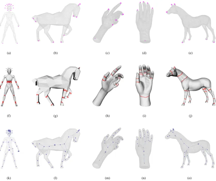
(a) (b) (c) (d) (e)
(f) (g) (h) (i) (j)
(k) (l) (m) (n) (o)
Figure 12. Feature points, constriction approximations and enhanced topological skeletons of stan-dard models.
Model Faces Feature pts. Constrict. Time Humanoid 1 900 19 9 0.5 s. Horse 1 20 000 10 11 12 s. Hand 1 50 000 6 11 75 s. Hand 2 50 000 6 11 100 s. Horse 2 40 000 7 19 35 s.
Table 2. Computation times.
8.1. Discussion
Figure 12 presents intermediary results and enhanced topological skeletons of standard models.
Firstly, we can notice that our feature point extraction algorithm achieves correct extractions, even on complex ar-eas, such as the hair of the humanoid model.
Secondly, our constriction approximation algorithm computes nice-looking constrictions (in red in fig. 12) even for coarsely designed objects (figs. 12(f) and 12(g)). It au-tomatically adjusts its detection criterion to the connected component it is processing, enabling the identification of constrictions even on strongly tubular mesh sub-parts (like the legs of the horse models).
Table 1 shows that the number of identified constrictions is quite stable whenfτvaries. The most visually interesting
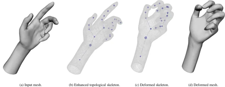
(a) Input mesh. (b) Enhanced topological skeleton. (c) Deformed skeleton. (d) Deformed mesh.
Figure 13. Application to mesh deformation.
results have been obtained settingfτ= 10. This setting has
been chosen for each model in fig. 12.
However, constrictions are approximated assuming they appear along identified discrete contours only. This is a strong hypothesis. As shown in figure 12, thanks to our mapping function definition, this limitation is not detrimen-tal when dealing with natural objects because some con-tours are actually identified on the articulations of promi-nent compopromi-nents.
Constriction approximation leads to the subdivision of the branches of the topological skeleton into more visually interesting parts: such as the decomposition of fingers into phalanxes (figs. 12(m) and 12(n)) or the decomposition of legs into thighs, calves and feet (figs. 12(k), 12(l) and 12(o)).
Thanks tofminvariance properties, those skeletons are
invariant to geometrical transformations: translation, rota-tion and uniform scaling. Furthermore, as shown secrota-tion 6, thanks to our graph construction strategy, no noisy details are encoded in the skeletons.
8.2. Time complexity
Given an input connected triangulated surface T , let n be the number of vertices in T . Feature point extrac-tion is performed in O(n × log(n)) steps. fm is
com-puted inO(|F | × n × log(n)) steps with |F | the number of identified feature points. Notice that fm has a lower
computational cost than the function proposed in [10] (|F | rarely exceeds 20). Each discrete contour computation takes O(log(n) + n). Therefore, as contours are computed for each vertex in T , the overall discrete contour computa-tion takesO(n2) steps. Topological and geometrical
anal-yses are more straightforward. Topological analysis is per-formed inO(n) steps. Concavity curves are computed in
O(n) steps. Their smoothing is realized in O(n × log(n)), using the Fast Fourier Transform algorithm. Consequently, we can state that the overall complexity of our method is bounded by the discrete contour computation, which takes O(n2) steps.
Presented algorithms have been implemented in C lan-guage under GNU/Linux and experimented on a desktop PC with a 3 GHz P4-CPU and 2 gigabytes of RAM. Table 2 shows the computation times corresponding to the mod-els presented in fig. 12. Notice that our overall method has a significantly lower running time than latest constric-tion detecconstric-tion [8] or skeleton extracconstric-tion [24] methods, for equivalently sampled meshes.
8.3. Example of application: mesh deformation
Topological skeletons have shown to benefit various ap-plications in computer graphics [2]. For example, within the framework of shape retrieval, thanks to their invariance properties, enhanced topological skeletons can be used for shape similarity estimation. They are also good supports for shape compression, metamorphosis, texture mapping, etc.
In this paper, to show the usability of our approach, we focus on mesh deformation. Each node of the enhanced topological skeletons references each vertex of the related mesh sub-component. Thus, a novice user can easily apply deformations on selected parts of the object.
Since mesh deformation is not in the scope of this paper, in our experiments, models are deformed by applying sim-ple rotations to components, but more sophisticated strate-gies can be used [13]. Given an angle and an axis of ro-tation, a rotation matrix is computed. Then it is applied to each vertex of the selected node, providing nice-looking de-formations, as shown in figures 1(f) and 13.
9. Conclusion and future works
In this paper, we presented a fully automatic algorithm for the extraction of affine-invariant enhanced topological skeletons. It first computes a dual Reeb graph. Then it re-fines it using constrictions as boundaries between mesh sub-parts. To our knowledge, this is the first approach which unifies Reeb graph and constriction computations.
Our scientific contribution resides in three points. Firstly, we proposed a robust and straightforward feature point ex-traction algorithm. It enables the computation of an invari-ant mapping function which reveals well the shape most significant features. Secondly, we presented an algorithm for discrete contours computation. We showed that a topo-logical analysis of these discrete contours enables a unified Reeb graph construction and simplification process. Result-ing graphs do not encode noisy details and they are robust against variations in mesh sampling and invariant to geo-metrical transformations. Finally, we showed that a geomet-rical analysis of the discrete contours provides nice-looking constriction approximations on prominent components, en-abling the refinement of dual Reeb graphs into more visu-ally meaningful skeletons.
Our algorithm computes skeletons with satisfactory exe-cution times, without any input parameter or pre-processing stage. Consequently, it is a good candidate for various ap-plications in computer graphics, like shape deformation (ex-perimented in this paper), retrieval, metamorphosis, com-pression, texture mapping, etc.
In the future, we would like to experiment more robust geometrical analyses and constriction sliding algorithms, in order to provide more visually interesting skeletons. More-over, forcing the position of the skeleton inside the object and preserving shape symmetry are enhancements which benefit certain applications and which are currently under investigation.
References
[1] M. Attene, S. Biasotti, and M. Spagnuolo. Shape under-standing by contour-driven retiling. The Visual Computer, 19:127–138, 2003.
[2] S. Biasotti, S. Marini, M. Mortara, and G. Patan`e. An overview on properties and efficacy of topological skeletons in shape modelling. In Shape Modeling International, pages 245–254, 2003.
[3] H. Blum and R. N. Nagel. Shape description using weighted symmetric axis features. Pattern Recognition, 10:167–180, 1978.
[4] P.-T. Bremer, H. Edelsbrunner, B. Hamann, and V. Pascucci. Topological hierarchy for functions on triangulated surfaces.
IEEE Transactions on Visualization and Computer Graph-ics, 10:385–396, 2004.
[5] H. Carr, J. Snoeyink, and M. V. de Panne. Simplifying flex-ible isosurfaces using local geometric measures. In IEEE
Visualization, pages 497–504, 2004.
[6] K. Cole-McLaughlin, H. Edelsbrunner, J. Harer, V. Natara-jan, and V. Pascucci. Loops in Reeb graphs of 2-manifolds. In Symposium on Computational Geometry, pages 344–350, 2003.
[7] H. Edelsbrunner and E. P. M¨ucke. Simulation of simplicity: a technique to cope with degenerate cases in geometric al-gorithms. ACM Transactions on Graphics, 9:66–104, 1990. [8] F. H´etroy. Constriction computation using surface curvature.
In Eurographics, pages 1–4, 2005.
[9] F. H´etroy and D. Attali. From a closed piecewise geodesic to a constriction on a closed triangulated surface. In Pacific
Graphics, pages 394–398, 2003.
[10] M. Hilaga, Y. Shinagawa, T. Kohmura, and T. Kunii. Topol-ogy matching for fully automatic similarity estimation of 3D shapes. In SIGGRAPH, pages 203–212, 2001.
[11] S. Katz, G. Leifman, and A. Tal. Mesh segmentation us-ing feature point and core extraction. The Visual Computer, 21:865–875, 2005.
[12] F. Lazarus and A. Verroust. Level set diagrams of poly-hedral objects. Technical Report 3546, Institut National de Recherche en Informatique et en Automatique (INRIA), 1999.
[13] J. Lewis, M. Cordner, and N. Fond. Pose space deforma-tions: A unified approach to shape. In SIGGRAPH, pages 165–172, 2000.
[14] M. Meyer, M. Desbrun, P. Schrder, and A. H. Barr. Dis-crete differential-geometry operators for triangulated 2-manifolds. In Visualization and Mathematics, pages 33–57, 2002.
[15] J. Milnor. Morse Theory. Princeton University Press, 1963. [16] M. Morse. Relations between the critical points of a real function of n independant variables. Transactions AM. Math. Soc., 27:345–396, 1925.
[17] M. Mortara and G. Patan`e. Affine-invariant skeleton of 3D shapes. In Shape Modeling International, pages 245–252, 2002.
[18] X. Ni, M. Garland, and J. Hart. Fair Morse functions for extracting the topological structure of a surface mesh. ACM
Transactions on Graphics, 23:613–622, 2004.
[19] G. Reeb. Sur les points singuliers d’une forme de Pfaff compl`etement int´egrable ou d’une fonction num´erique.
Comptes-rendus de l’Acad´emie des Sciences, 222:847–849, 1946.
[20] A. Shamir. A formalization of boundary mesh segmentation. In IEEE 2nd International Symposium on 3DPVT, 2004. [21] P. Shilane, P. Min, M. Kazhdan, and T. Funkhouser. The
Princeton shape benchmark. In Shape Modeling
Interna-tional, pages 167–178, 2004.
[22] Y. Shinagawa, T. L. Kunii, and Y. L. Kergosien. Surface coding based on morse theory. IEEE Computer Graphics
and Applications, 11:66–78, 1991.
[23] S. Takahashi, T. Ikeda, Y. Shinagawa, T. L. Kunii, and M. Ueda. Algorithms for extracting correct critical points and constructing topological graphs from discrete geograph-ical elevation data. Computer Graphics Forum, 14:181–192, 1995.
[24] F.-C. Wu, W.-C. Ma, R.-H. Liang, B.-Y. Chen, and M. Ouhy-oung. Domain connected graph: the skeleton of a closed 3D shape for animation. The Visual Computer, 22:117–135, 2006.