Dayside and nightside reconnection rates inferred from IMAGE FUV and Super Dual Auroral Radar Network data

1 2 3 4 5 6 7 8

Dayside and nightside reconnection rates inferred from

IMAGE-FUV and SuperDARN data

B. Hubert

, S.E. Milan

, A. Grocott

, C. Blockx

,

19

S. W. H. Cowley

, and J.-C. Gérard

20 21 22 23 24 25 26 27

1. Laboratoire de Physique Atmosphérique et Planétaire, University of Liège, Belgium

28

2. Department of Physics and Astronomy, University of Leicester, Leicester LE1 7RH, United Kingdom

29 30 31 32 33 34 35 36 37

Submitted for publication to Journal of Geophysical Research 38 39 March 2005 40 41 42

Abstract

1

The Spectrographic Imager at 121.8 nm (SI12) of the Far UltraViolet (FUV) 2

experiment onboard the IMAGE spacecraft produces global images of the Doppler-shifted 3

Lyman-α emission of the proton aurora. This emission is solely due to proton precipitation 4

and is not contaminated by dayglow, allowing us to monitor the auroral oval on the dayside as 5

well as on the nightside. Remote sensing of the polar aurora can be advantageously 6

supplemented by use of ground based data from the Super Dual Auroral Radar Network 7

(SuperDARN) that monitors the ionospheric convective flow pattern in the polar region. In 8

the present study, the SI12 images are used to determine the location of the open/closed field 9

line boundary, and to monitor its movement. The SuperDARN data are then used to compute 10

the ionospheric electric field at the location of the open/closed boundary. The total electric 11

field is then computed along the boundary accounting for its movement via Faraday’s law, so 12

that the dayside and nightside reconnection voltages can be derived. This procedure is applied 13

to several substorm intervals observed simultaneously with IMAGE-FUV and SuperDARN. 14

The dayside reconnection voltage feeds the magnetosphere with open flux, which is later 15

closed by nightside reconnection. The calculated dayside reconnection rate is consistent with 16

the solar wind properties measured by the Geotail, Wind, and ACE satellites. We identify the 17

presence of nightside reconnection due to pseudobreakups taking place during the growth 18

phase. In several cases, we establish that the nightside reconnection rate is maximum at the 19

time of the substorm expansion phase onset or shortly after, reaching ~120 kV, and then 20

slowly returns to undisturbed values of ~30 kV. The flux closure rate can also start 21

intensifying prior to expansion phase onset, producing pseudobreakups. 22

1. Introduction

1

In 1961, Dungey published a pioneering work sketching the general dynamics of the 2

Earth’s magnetic field line interaction with the solar wind [Dungey, 1961]. The “Dungey 3

cycle” describes how field lines of the planetary magnetic field are opened at the dayside 4

magnetopause by reconnection with the interplanetary magnetic field carried by the solar 5

wind, are convected antisunward by the solar wind flow, then reconnect in the nightside tail 6

thus returning to a closed topology, and are finally convected back to the dayside. The four 7

steps of this cycle take place simultaneously in the magnetosphere almost all the time, 8

creating the polar ionospheric convection. Cowley and Lockwood [1992] and references 9

therein summarized how the sign of each IMF component influences the dayside reconnection 10

and the convection flow pattern. In particular, significant magnetic flux opening is expected 11

when the IMF Bz component is southward (i.e. negative), but becomes greatly reduced when

12

the IMF points northward. 13

The opening of magnetic flux at the dayside creates the necessary conditions to produce 14

substorms via an accumulation of open magnetic flux and hence field energy in the magnetic 15

tail. The period of time preceding a substorm expansion during which the magnetosphere 16

“accumulates” open magnetic flux is often referred to as the growth phase. This phase is 17

characterized by an increase in radius of the auroral oval. During subsequent substorm 18

expansions, magnetic field lines that have previously been opened at the dayside and 19

convected downtail by the solar wind reconnect within the tail plasma sheet, causing a 20

substantial flux closure which releases accumulated field energy to the plasma particles. This 21

reconfiguration of the tail magnetic field takes place together with poleward-expanding 22

auroral particle precipitation, and modification of the electric field, plasma flow, and currents 23

flowing in the coupled magnetosphere-ionosphere system. 24

Both dayside and nightside reconnection of field lines are associated with potential 1

drops across the open/closed field line boundary, as can be understood by considering 2

Faraday's law, as expressed in equation (1) (Siscoe and Huang, 1985; see also Grocott et al., 3

2002, Milan et al., 2003, 2004, Milan, 2004 and references therein). Changes in the amount of 4

open flux threading the polar cap Φ are related to the total electric field E r by the expression: 5 ∫ ⋅ − = _CEdl dt dΦ r r_{, (1)} 6

where C is the curve encircling the polar cap area S, and the open magnetic flux is 7 ds n B Φ r r ⋅ =

_∫

nr being the vector normal to the area S, and B r

the Earth’s magnetic field. The electric field 9

E r

must be computed in the frame of reference moving with the boundary C and is thus 10 B v E E _i r r r r × + = , (3) 11 where E_i r

is the ionospheric electric field measured in a frame of reference fixed with respect 12

to the planet, and vr is the velocity of the moving boundary C (normal to the boundary). 13

Equation (1) relates to the rate of change of open flux in the system, equal to the 14

difference between the rate of open flux production at the magnetopause and open flux 15

closure in the tail. If these two rates are equal, for example, such that the amount of open flux 16

is constant, then the line integral of the electric field around the boundary will be zero, as it is 17

for any fixed closed contour containing a fixed amount of ionospheric magnetic field. When 18

both the boundary motion and ionospheric flow (related to the electric field) are known, it is 19

possible to obtain the rates of flux opening and flux closure separately. This can be done by 20

integrating the electric field in the boundary frame around those segments of the boundary 21

where flux is added to the open region, giving the “dayside” (or magnetopause) reconnection 1

rate, and where it is removed, giving the “nightside” (tail) reconnection rate. This is the task 2

undertaken in this paper. 3

The position of the polar cap boundary and its motion can be determined using space-4

borne imaging instruments giving a global view of the auroral morphology, with the poleward 5

limit of the auroral oval identified with the open/closed boundary. The ionospheric electric 6

field can be determined from knowledge of the ionospheric convection flow pattern as 7

determined, for instance, with the Super Dual Auroral Radar Network, using the method of 8

Ruohoniemi and Baker [1998] to derive the electric field and potential across the whole polar 9

cap. The flow velocity vr_i and the ionospheric electric field are related to each other through 10 B v E_{i i} r r r × − = . (4) 11

The convection flow pattern shows how newly opened field lines are introduced into the polar 12

cap on the dayside, and are convected towards the nightside across the polar cap. It also 13

shows how closed field lines are redistributed and convected back from the nightside to the 14

dayside outside of the polar cap after nightside reconnection. In some circumstances, it is also 15

possible to use the characteristics of the radar backscatter signal to infer the location of the 16

open-closed field line boundary and to follow its motion [Milan et al., 2003, and references 17

therein]. However, the boundary position is not always unequivocal in such data, while 18

generally the whole of the boundary is not observed due to limitations of radar coverage. 19

Chisham et al. [2005] nevertheless showed from a statistical standpoint that the Spectral 20

Width Boundary (SWB), the boundary between broad and narrow backscatter echoes, is a 21

reliable proxy for the open/closed boundary close to noon and midnight. Note also that 22

Chisham et al. [2004] measured the dayside reconnection rate during an interval of northward 23

IMF combining SuperDARN and DMSP data. 24

Blanchard et al. [1996, 1997a] developed a method to determine the local nightside 1

reconnection rate using ground based measurements of the emission of metastable oxygen 2

O(1D) at 630 nm combined with radar measurement of the ionospheric flow, and applied it to 3

the study of several substorms [Blanchard et al., 1997b]. They found that the nightside 4

reconnection rate increases shortly after substorm onset. This method however suffers from 5

its spatial limitation, sometimes also introducing a time delay between the expansion phase 6

onset and the measurement of the increase of the reconnection rate at some distance from the 7

location of the onset. In addition, the auroral oxygen red line emission at 630 nm is strongly 8

contaminated by the dayglow (the dissociative recombination of O2+ produces metastable

9

oxygen), so that summer time studies are more difficult. This method is also generally 10

inapplicable to the determination of the dayside reconnection rate due to this contamination, 11

except perhaps in winter when the auroral oval is well separated from the dayside terminator. 12

Østgaard et al. [2005] combined FUV images of the electron aurora with radar 13

measurement from EISCAT to estimate the magnetotail reconnection rate, and found an event 14

presenting a bursty reconnection electric field. These authors also summarised how the 15

ionospheric electric field estimated along the open/closed boundary can be related to the field 16

at the reconnection site, after the work of Vasyliunas [1984]. 17

In the present paper, we employ IMAGE-FUV data to determine the morphology of the 18

auroral oval and thus of the polar cap boundary on the global scale, combined with the 19

ionospheric electric field deduced from the SuperDARN flow patterns, to compute the total 20

open magnetic flux and the dayside and nightside reconnection rates. We propose a method 21

capable of determining these quantities at any time of the year. The method is applied to study 22

the temporal development of several substorms. The next section describes the method and 23

data that are used. The third section discussed some uncetainties and tests the accuracy of our 24

method in comparison with boundary identification using DMSP in situ particle 1

measurements while the fourth section presents the results obtained for several substorms. 2

Section 5 then discusses the uncertainties of the method. The main results are summarized in 3

section 6. We show that the nightside flux closure is maximum at the time of substorm onset 4

or shortly after, and that pseudobreakups taking place during the growth phase significantly 5

increase the nightside closure voltage prior to onset. 6

2. Instrumentation and analysis techniques.

7

The IMAGE satellite was launched on 25 March 2000 into an eccentric orbit with an 8

apogee of ~7 RE, a perigee of ~1000 km, and an orbital period of ~14 h. The FUV experiment

9

[Mende et al., 2000 a, b] includes three imagers of interest here, that generate an FUV image 10

of the Earth every two minutes (the period of the rotation of the satellite on its axis). The 11

Wide Band Imaging Camera (WIC) observes the N2 LBH bands between 135 and 180 nm, the

12

first channel of the Spectrographic Imager (SI13) is centred on the OI 135.6 nm transition, 13

while the second channel of the Spectrographic Imager at 121.8 nm (SI12) observes the 14

Doppler-shifted Lyman-α emissions due to the proton aurora. The geocoronal Lyman-α 15

component at the rest wavelength 121.6 nm is efficiently rejected by the instrument, as well 16

as the nearby NI 120 nm line. The WIC and SI13 cameras globally image emissions mostly 17

produced by precipitating electrons. The additional contribution due to proton precipitation 18

and the secondary electrons they generate can be obtained on the basis of the SI12 19

measurements. The snapshots taken simultaneously once every two minutes by the WIC, 20

SI13, and SI12 imagers are well suited to a study of the dynamics, morphology and energetics 21

of the global electron and proton precipitation. 22

The data used to determine the polar cap boundary are the images of the proton aurora 23

obtained with the IMAGE-FUV SI12 imager. A threshold can be determined for each image 24

individually on a statistical basis, to discriminate between the auroral signal and the image 1

background. This threshold must be accurately determined, as the boundary sought 2

corresponds to the limit where the auroral emission drops to zero. The SI12 images are 3

preferred to SI13 and WIC, despite the higher sensitivity of the latter camera, and to a lesser 4

extent the SI13 camera, since these cameras are more subject to dayglow contamination. This 5

arises because the mechanisms producing the bulk of the auroral emissions and the dayglow 6

emissions are similar. The Doppler-shifted Lyman-α emission does not suffer from this 7

drawback because these photons are emitted directly by the precipitating protons capturing an 8

electron. SI12 images are never significantly contaminated by dayglow emissions and are thus 9

well suited to a systematic determination of the auroral emission boundary. Indeed, in the 10

present study, this issue is critical since the residual noise following dayglow subtraction must 11

not be confused with the auroral signal, as we seek to identify the boundary of the auroral 12

emission. However, for periods close to the winter solstice when dayglow is confined to lower 13

latitudes near noon, the separation of the electron aurora from the dayglow is often 14

unambiguous, especially when the polar cap is small, giving us the opportunity to compare 15

the open flux determined with the SI12, SI13, and WIC imagers. In addition, Sergeev et al. 16

[1983] showed that the chaotization of the velocity distribution of the trapped protons feeding 17

the proton aurora is due to the violation of the first adiabatic invariant on the closed stretched 18

field lines of the magnetotail. It is thus legitimate to consider that significant proton 19

precipitation occurs along closed field lines. We can thus expect to use the poleward limit of 20

the proton aurora to set up a reasonable proxy for the open/closed field line boundary.This is 21

however a nontrivial problem subject to uncertainties, which is affected by sensitivity 22

threshold issues. 23

The Super Dual Auroral Radar Network (SuperDARN), also used in this study, collects 24

data from nine radars in the northern hemisphere (eight radars during the period of interest). 25

The radar pulses scatter from naturally-occuring irregularities in the ionospheric plasma, the 1

time delay between emission and echo giving the location of the scattering volume, and the 2

Doppler shift of the echo giving the velocity of the plasma perpendicular to the field lines 3

along the line of sight. Ruohoniemi and Baker [1998] developed the “Map-Potential” method 4

to reconstruct the ionospheric convection pattern and the associated electric field using the 5

ensemble of line-of-sight velocity values available from all the SuperDARN radar operating 6

during a particular interval. The electric potential is expressed as a series of spherical 7

harmonics whose coefficients are determined using a least squares fit technique applied to the 8

measured component of the flow velocity. A statistical model of the ionospheric convection 9

flow is also used [Ruohoniemi and Greenwald, 1996], that accounts for the interplanetary 10

properties when they are known, allowing to constrain the fitted potential over areas of the 11

polar region where no data are avilable. The method is conceived such that as little 12

information as necessary is introduced from the model to prevent the fitted potential from 13

having an unrealistic behaviour [Ruohoniemi and Baker, 1998]. As pointed out by Grocott et 14

al. [2002] when data are missing over an active portion of the oval, during the expansion 15

phase of a substorm for example, the fitted potential can be less reliable over that part of the 16

oval, since the model used to constrain the least squares fit in that area represents an 17

‘averaged’ situation rather than the specific conditions prevailing for a particular event, which 18

may depart from the average in the active portion of the oval at that time. In the present study, 19

we selected intervals with a good SuperDARN coverage to reduce the effect of potentially 20

inaccurate input from the model used to constrain the “Map-Potential” method in the 21

uncovered areas. 22

In the analysis presented here, the poleward boundary of the auroral oval is identified 23

from the IMAGE-FUV SI12 data as indicated above, fitted with a Fourier series, and its 24

velocity determined from the displacement in successive images. The fitting of the boundary 25

with a Fourier series is necessary to extrapolate the boundary in regions where the proton 1

aurora is not bright enough to be detected with the SI12 instrument. A series of five 2

harmonics is generally used. Using more harmonics in the series would increase the risk of 3

having local artificial oscillations that would impair the quality of the physical results. In 4

addition, the time derivative is very easy to compute numerically when it is expressed with a 5

Fourier series, only the coefficients of the series being dependant on time. The total electric 6

field in the frame of reference of the boundary can then be computed by combining these 7

results with the electric field of the ionospheric flow from the SuperDARN data. Faraday's 8

law is then applied to compute the opening (dayside) and closing (nightside) potential drops, 9

integrating the electric field across the moving boundary. Regions of positive (negative) Edl r r

⋅ 10

were considered as threading the dayside (nightside, respectively) reconnection site. Note that 11

the net contribution of the electric field associated with the ionospheric flow to the rate of 12

change of the open magnetic flux is zero, since it represents the voltage across a closed static 13

loop. Nevertheless, this electric field cannot be neglected when computing the nightside and 14

dayside reconnection voltages separately. 15

For validation purposes, we concentrate on a restricted set of data collected during the 16

winter season in 2000 when an adequate coverage of the auroral region is guaranteed both for 17

the IMAGE-FUV and SuperDARN data. These time intervals contain at least one substorm 18

whose onset has been observed in the IMAGE-FUV data. Using these data, we then study 19

both the period when the polar cap expands due to significant dayside reconnection and weak 20

nightside reconnection, and the following period of intense flux closure on the nightside 21

during substorms. 22

23

3. Reliability of the boundary determination.

1

As mentioned before, the advantage of using the SI12 images of the proton aurora to 2

estimate the location of the open-closed field line boundary is the absence of dayglow 3

contamination, so that global coverage can be achieved on the nightside and dayside at any 4

time of the year, for any size of the auroral oval. It nevertheless suffers some limitation. Due 5

to the sensitivity threshold, proton precipitation along the polwardmost field lines may be too 6

weak to produce Lyman-α emission detectable with SI12, biasing the location of the boundary 7

equatorward. This would result in an overestimation of the open magnetic flux. As a side 8

effect, when the oval suddenly brightens, areas previously threaded by closed field lines 9

located poleward of the optical boundary may light up in the detector, resulting in an artificial 10

poleward motion of the boundary. It is thus necessary to clarify the relation linking the optical 11

SI12 poleward boundary and the open/closed field line boundary. As this source of error 12

depends on the auroral brightness through the instrument detection threshold, it is natural to 13

search for a correction that depends on the SI12 count rate. 14

We compared the location of the SI12 poleward boundary with the location of the b5e, 15

b5i and b6 boundaries determined with the DMSP in situ particle flux data. We also 16

conducted a comparison with the open/closed field line boundary deduced from the 17

classification of particle regimes using the DMSP in situ measurements (which we will note 18

as ‘boc’ when deduced from DMSP particle measurements) as decribed by Newell et al. 19

[1991], and as was done by Blanchard et al. [1997]. DMSP b5e and b5i correspond to the 20

location where the flux and/or energy of electrons and protons, respectively, drop abruptly. 21

Boundary b6 is the poleward limit of the auroral drizzle. The boc boundary is identified when 22

a transition is observed in the origin of the precipitating particles from a known closed region 23

to a known open region of the magnetosphere. The b5e and b5i limits are generally close to 24

each other on the spatial scale of interest in the present problem (the size of an SI12 pixel 1

projected on the planet surface is roughly 1° MLAT). Although weak proton precipitation can 2

be measured in the drizzle between the b6 boundary and the polewardmost b5 boundary, this 3

does not guarantee that all these field lines are closed (P. T. Newell, personal communication, 4

2005). For completeness, we conducted a statistical study comparing the location of the b5e, 5

b5i and b6 boundaries with the open/closed field line boundary inferred from the systematic 6

dayside classification of polar regions based on the DMSP particles measurements, i.e. boc 7

[Newell et al.,1991]. The difference between the magnetic latitude of the boc boundary and of 8

the b5i (b5e, b6) boundary is on average 1.45° ± 0.055° (1.22° ± 0.058° , -1.15° ± 0.057°, 9

respectively), the standard deviation of this difference being 2.75° (3.17°, 2.81°, respectively). 10

We also compared the average value (MLATb5i + MLATb6)/2 with the latitude of the DMSP

11

boc boundary and found that the difference between these two is on average 0.02° ± 0.069°, 12

with a standard deviation of 2.45°. We conclude that the open/closed field line boundary 13

deduced from the DMSP classification lies midway between the b5i and b6 boundaries on 14

average. Both the b5i and b5e boundaries are a little more than a degree equatorward of the 15

boc boundary, while the b6 boundary is 1.15° poleward of the boc. This value can be 16

compared with the spatial resolution of spaceborn global imagers. In a previous study, Baker 17

et al. [2000] compared the latitude of the b5e boundary with Polar UVI data, and found the 18

b5e boundary lies 1° poleward of the optical boundary determined by POLAR-UVI. Our 19

study thus suggests that the boc boundary lies on the order of ~2.5 degrees poleward of the 20

POLAR-UVI boundary, on average. Note also that Blanchard et al. [1995, 1997a] used the 21

DMSP classification to calibrate their method of determination of the open-closed boundary 22

based on the meastable O(1D) emission at nighttime, and estimated an accuracy of 0.9° 23

invariant latitude. 24

Our study compares the optical boundary of the proton aurora as seen with IMAGE-1

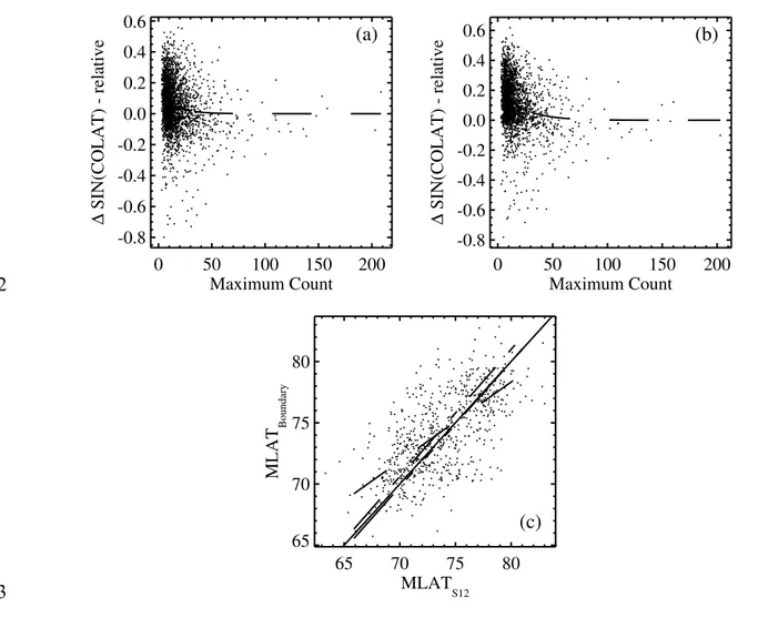
FUV SI12 with the DMSP boundaries. Figure 1 summarizes our comparison between the 2

DMSP boundary locations and the optical boundary of the proton aurora. We compare the 3

SI12 proton optical boundary and the b5e (not shown), b5i, b6 and boc boundaries. Let r be 4

the sine of the colatitude of the boundary, i.e. the radius of the boundary projected in the 5

equatorial plane. We fitted a decreasing exponential function on the relative difference (rSI12 –

6

rDMSP) / rSI12 as a function of the maximum SI12 count measured in a 1h MLT sector centred

7

on the location of the DMSP boundary. Despite some scatter, the bulk of the data show that 8

when the aurora is bright, the SI12 and DMSP b5e, b5i and b6 boundaries match each other 9

fairly well. At lower count rates, a correction should be applied, based on the exponential 10

function fitted to the data, representing the average discrepancy between the optical boundary 11

of the proton aurora and the DMSP b5i and b6 boundaries. Surprisingly, no such relation 12

could be established between the maximum count rate and the difference of the boc and SI12 13

boundary locations. Instead, we found that the boc boundary lies on average 0.55° ± 0.093° 14

poleward of the SI12 boundary (standard deviation: 2.76°). It must be noted that the boc 15

boundary location differs in nature from the b5e, b5i and b6 boundaries. While the b5e, b5i 16

and b6 boundaries rely on quantitative variations of the precipitating flux, the boc boundary 17

relies on the properties of the spectrum of the precipitating particles, allowing their 18

magnetospheric origin to be identified. It is thus intuitively natural that the SI12 boundary 19

relates to the b5 and b6 boundaries through the quantitative properties of the aurora, whereas 20

the relation with the boc location does not necessarily need to. Note in addition that the 21

regression line fitted to the data in Figure 1c (dashed line) does not match the bisector (solid 22

line), but a best line minimizing the maximum distance between the data and the fitted line 23

(dash-dot-dot-dot line) is very close to the bisector, whereas the best line minimizing this 24

distance in a least squares sens (dash-dot line) is roughly parallel to the bisector at a distance 25

roughly reflecting the average difference between both variables. We thus correct the location 1

of the SI12 boundary by a fixed amount of ~0.55° and retrieve a more reliable estimate of the 2

location of the open-closed field line boundary, in an average sens. Note that the geometry of 3

the DMSP orbit is such that most of the data were acquired in the 18 – 24 MLT sector, and 4

care should be taken in extrapolating the result to other MLT sectors. Nevertheless, there is no 5

obvious reason to believe that the relation between boundary locations should be dramatically 6

different in the 0 – 6 MLT sector, considering that this difference essentially relies on 7

sensitivity limitations. The situation may be more critical around the noon sector, which has 8

the additional complication that the cusp region is generally bright in the SI12 images, 9

although it is threaded by open field lines. Consequently, we do not apply any correction in a 10

1 hour MLT sector centred on the noon sector, in an attempt to avoid worsening this bias. 11

One drawback of using auroral data to identify the OCB is that while most aurora 12

appear on closed field lines it is well known that the cusp aurora are on open field lines, so 13

our technique underestimates the amount of open flux in the polar cap. However, we will now 14

discuss why we feel that this introduces only a minimal error to the deduced reconnection 15

rates. It is easily shown that, providing the orientation of the tangential (with respect to the 16

boundary) component of the ionospheric electric field only varies slightly versus latitude on 17

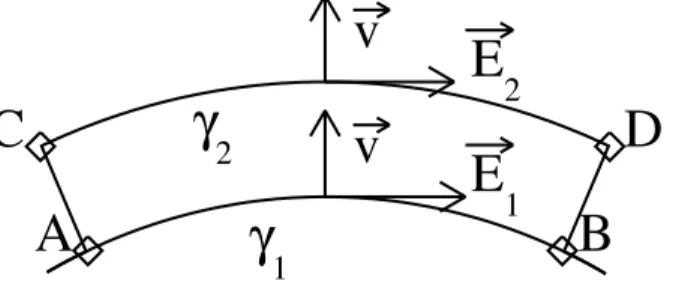
the scale of a few degrees, the shape of the moving boundary in the cusp region is not crucial 18

for the computation of its contribution to the reconnection rate. Assuming that the sign of E t r r ⋅ 19 (with t r

the unit vector tangent to the boundary) does not change along paths γ1 and γ2

20

described in Figure 2 , the voltage between points A and B does not depend on the path 21

chosen to integrate E t r r

⋅ , so that the net voltage can be computed integrating along any path. If 22

no significant flux closure takes place along field lines threading the noon sector, the 23

contribution of the ionospheric electric field to the flux opening rate is reliably computed 24

independent of the detail of the integration path in the noon sector. Considering now the 1

motion of the boundary, the electric field responsible for the reconnection rate is the second 2

term of rhs of equation 3. Considering the open-closed boundary moves equatorward at 3

velocity v (Figure 2), one can compute the motional voltage between points A and B along 4

paths γ1 and γ2 . Assuming a dipole field of magnetic moment M, and noting the colatitude

λ

5

the magnetic permeability µ0 and the planet radius (at ionospheric altitude) R , the magnitude

6

of the electric field is 7 ) sin( 2 3 0

λ

π

µ

and the motional voltages V1 and V2 between A and B (separated by an angle ∆ϕ) along paths

9

γ1 and γ2 respectively are

10 ) ( sin 2 M V 0 ₂ 2 1

λ

π

µ

ϕ

λ

δλ

π

µ

ϕ

assuming that both paths are δλ apart in colatitude, so that the relative difference 11

(V2 – V1) / V1 is (sin2(λ+δλ)-sin2(λ))/sin2(λ). At 70° MLAT, λ=20° and a difference δλ=1° in

12

colatitude translates to a relative difference of ~10% in the motional voltage computed 13

between points A and B (in other words, V 2cot ( ) 0.096 V 1 _{= ≈} ∂ ∂

_δλ

_λ

_δλ

λ

i.e. at MLAT = 80°, the error computed in the same way is ~20%. The impact on the total flux 15

opening voltage computed in the cusp sector will depend on the relative contribution of the 16

convection and motional electric fields to the potential drop. As the convection velocity is 17

generally larger than the velocity of the motion of the boundary in the cusp sector, we can 18

estimate a typical value of the relative error made on the flux opening voltage computed in the 1

cusp sector by neglecting the detailed shape of the cusp when the ionospheric and motional 2

voltages are equal: it ranges from ~5% at 70° MLAT to ~10% at 80° MLAT. Smaller errors 3

will be made when the convection velocity is larger than the boundary motion velocity. 4

Larger errors may however occur when the convection is weak and the motion of the 5

boundary is large. The maximum relative error is obtained assuming that the ionospheric 6

electric field is zero, i.e. only the motional electric field contributes to the reconnection 7

voltage, and ranges from 10 % at 70° MLAT to 20% at 80° MLAT, as computed before. As 8

already stated above, these errors refer to the systematic bias inherant to the mislocation of the 9

open/closed field line boundary in the cusp sector only. 10 11

4. Case Studies

4.1. 26 December 2000

We first study the interval starting at 1715 UT on 26 December 2000 and ending at 14

0244 UT on 27 December 2000. During this 9 h 30 min period, the SI12 instrument made 15

continuous observations of the northern polar region. Simultaneously, the SuperDARN radar 16

network obtained measurements of the ionospheric convection pattern, so that the ionospheric 17

electric potential and electric field can be retrieved. In addition, the Geotail satellite was 18

ideally positioned to measure the solar wind properties upstream of the Earth’s 19

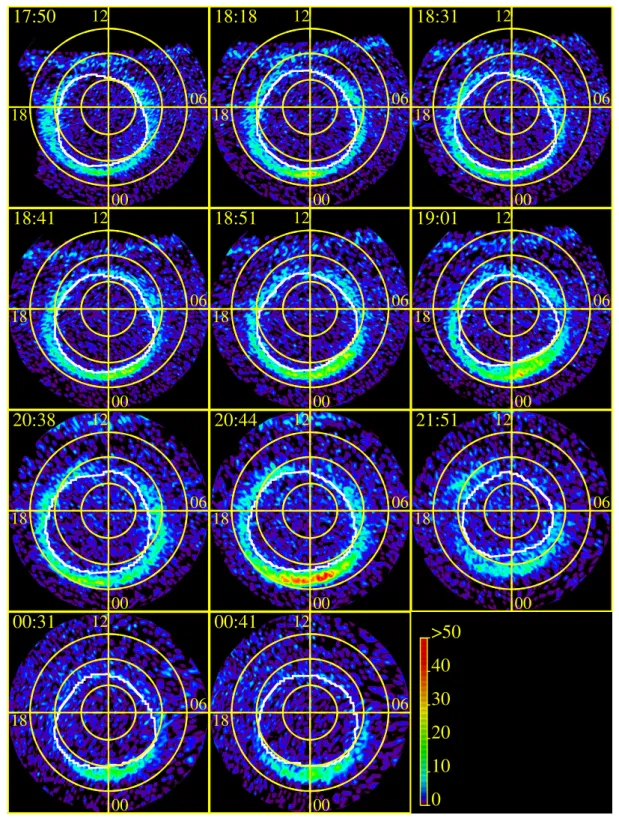
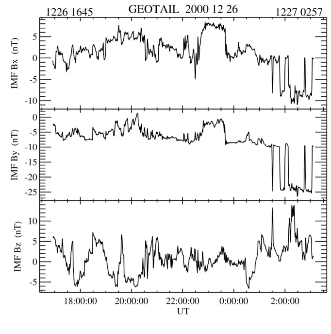
magnetosphere. Figure 3 presents a set of IMAGE SI12 snapshots obtained during the 20

interval, shown in a polar projection. This interval was preceded by a very long (more than 12 21

hours) period of negative IMF By, displacing the northern auroral oval to the dusk side by an

22

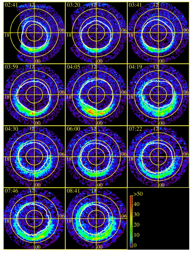
exceptionally large shift. The fitted polar cap boundary is overlaid as the continuous white 23

line. This fitted boundary does not strictly follow the image boundary, as it results from a 1

least-squares fit, but it nevertheless gives a very good overall representation of the boundary. 2

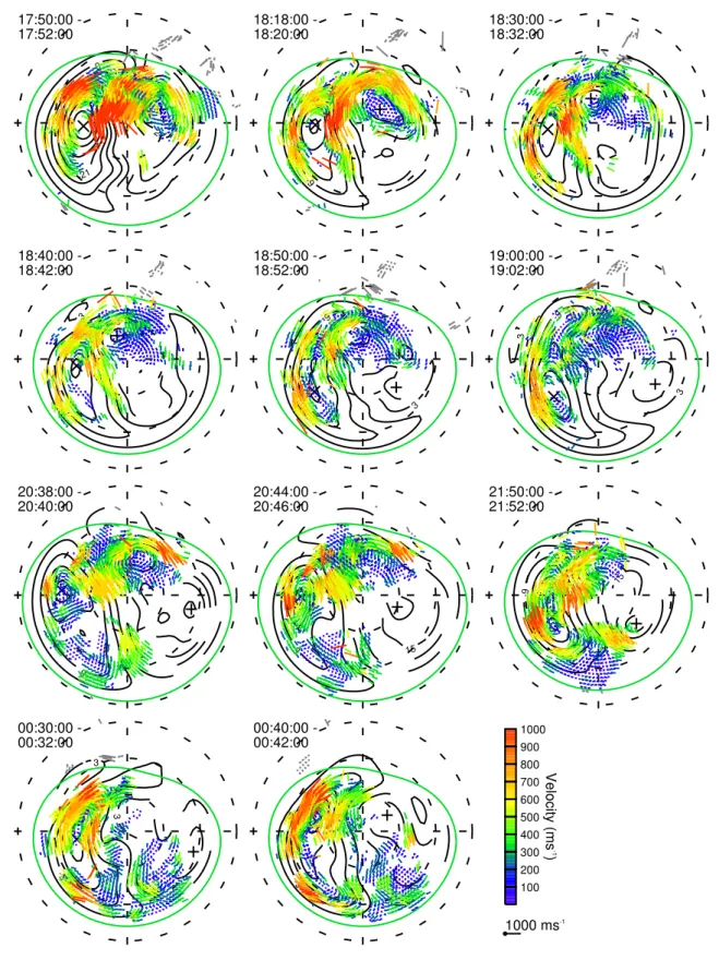
The simultaneous flow and electric potential patterns obtained with the SuperDARN network 3

(data accumulated over 2 min intervals) are presented in Figure 4. Velocity vectors are 4

reconstructed consistently with the fitted electric potential. The coverage of the polar region is 5

incomplete due to the absence of radar coverage in the Siberian sector of the polar region, so 6

that the electric potential pattern is completed using the technique of Ruohoniemi and Baker 7

[1998]. Figure 5 also shows the solar wind properties as measured by the Geotail satellite 8

during the period of interest. The satellite crossed the bow shock after 0130 UT, and those 9

data should be used with care. 10

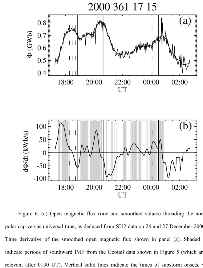
The open magnetic flux Φ was computed for each SI12 image obtained during the 11

interval. Its time derivative can then be computed directly following appropriate smoothing of 12

the curve. The smoothing is realised using a series of boxcar-average smoothings of 13

decreasing width. Investigation showed that this method produces results similar to Gaussian 14

smoothing and to digital filtering. The advantage of our method is that it rigorously conserves 15

both the low frequency shape and the integral of the smoothed function, which may not be the 16

case with the other methods when applied to an interval of finite size. Both the computed 17

magnetic flux and its derivative are shown in Figure 6. The noisy variations about the 18

smoothed curve a give an idea of the reliability of the method; uncertainties appear to be 19

lower than ~10%. 20

We verified that the open flux value deduced from the SI12 images is often smaller than 21

that deduced from the SI13 images (not shown). This indicates that our estimate of the auroral 22

limit using SI12 data is more accurate, since less equivocal identification of where the auroral 23

signal drops to zero is expected usually to lead to smaller open flux estimates. We also 24

verified that the open flux values deduced from the WIC images (not shown) often agree well 1

with the SI12 values, except for some periods where these values significantly depart from 2

each other, the value deduced from WIC being generally the larger. The quality of the Φ 3

values deduced from WIC images strongly decreases (sometimes giving unrealistic values) 4

when the auroral oval is weak on the dayside, such that the inferred boundary expands and 5

approaches the terminator. This tends to indicate that the Φ values deduced from SI12 images 6

are the most reliable, even during winter time. We attribute this higher reliability not to higher 7

sensitivity, but rather to the fact that the SI12 images can be more simply analysed and 8

interpreted. 9

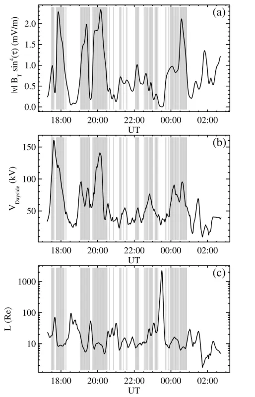
Returning to Figure 6, we note that the shaded intervals in Figure 6b correspond to 10

intervals of southward IMF, i.e. to intervals where significant dayside reconnection rate can 11

be expected, although moderate dayside reconnection can also occur during intervals of 12

positive IMF Bz, especially when appreciable IMF By is also present. These southward IMF

13

intervals are seen to match periods of positive derivative of Φ, unless significant nightside 14

reconnection also takes place. Pseudobreakups and substorm onsets can easily be identified 15

using the FUV imagers [Gérard et al., 2004], especially the WIC and SI13 instruments. 16

Substorm onsets and pseudobreakups often appear less clearly in the SI12 images. The 17

accuracy of the timing of the identified features is of course limited by the time resolution of 18

the FUV images, i.e. two minutes. Pseudobreakups are identified as a brightening initiated in 19

a localised portion of the auroral oval, similar to an expansion phase onset, but that does not 20

evolve into an expansion phase. They differ from poleward boundary intensifications (PBIs), 21

such as those presented in Figure 2 of Lyons et al. [2002], both in location and morphology. 22

At the start of the interval, Φ increases until ~1817 UT, when a first pseudobreakup takes 23

place, followed by two other pseudobreakups at 1831 and 1841, and a weak substorm onset at 24

1851 UT. The times of the pseudobreakups are indicated in Figure 6b by the vertical dashed 25

lines, while the substorm onsets are shown by the vertical solid lines. Note also that the SI12 1

images and SuperDARN data obtained at times discussed in this paragraph are shown in 2

Figures 3 and 4. The onset develops into a short-lived substorm-like event fading after ~1915 3

UT. Φ then increases again until ~2038 UT, when a further substorm onset takes place, 4

resulting in enhanced auroral FUV emission. The substorm auroral brightness progressively 5

fades after 2150 UT, and Φ starts increasing once more until ~0031 UT (27 December 2000) 6

when a third substorm onset is observed, followed by bright auroral emission and nightside 7

flux closure. 8

Throughout this interval, SuperDARN data coverage was sufficient to allow reliable 9

measurement of the ionospheric velocity over an extended area of the northern polar region, 10

from which the associated electric field and potential can be determined. The dayside and 11

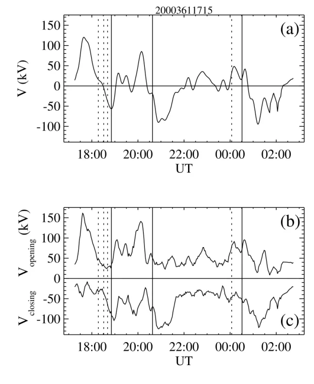
nightside reconnection rates were then calculated using the method described above in 12

sections 1 and 2. These are presented in Figure 7, together with their net value (i.e. the total 13

rate of change of open flux). Note that the net reconnection rate computed by applying 14

Faraday's law and by deriving Φ versus time (shown in Figure 6b) are identical, as expected 15

from Maxwell's equations, so that internal consistency is guaranteed despite the potential 16

sources of numerical errors. Also, the calculated nightside and dayside reconnection rates 17

associated with the flow itself actually cancel each other as expected, since their sum 18

represents the potential drop across a static closed loop. The period of rapid growth of Φ 19

between 1730 and 1815 UT (see figure 6) is characterized by intense dayside convection flow 20

into the polar cap with flow speeds sometimes exceeding 1000 m s-1 locally, indicating that 21

dayside reconnection is feeding the polar cap with open flux. The nightside “return” flow 22

speeds range between ~300 and ~650 m s-1 with a few local excursions above 700 m s-1. This 23

relatively high return flow speed is due to an expansion of the region of open flux into the 24

nightside, rather than to an increase in the nightside reconnection rate, as is shown in Figure 6 25

and also in Figure 7.The period of time rich in pseudobreakups extending between ~1815 and 1

~1850 UT has dayside convection velocities peaking at ~800 m s-1 at 1820 UT, then falling to 2

~600 m s-1 at 1850 UT in the centre of the polar cap, and with variable nightside return 3

convection velocities reaching ~600 m s-1, as directly measured in the dawn sector, related to 4

episodes of flux closure in the nightside magnetosphere. The size of the polar cap was non-5

increasing during that time interval, as can be seen in Figure 6. The following interval sees the 6

open flux increasing again, with significant dayside convection driving newly opened field 7

lines into the polar cap at speeds up to ~600 m s-1. The open flux increases more steeply after 8

~1950 UT, indicating intense dayside reconnection (see Figure 7). After the substorm onset 9

taking place at 2038 UT, the nightside return convection flow remains moderate, with the 10

open/closed field line boundary retracting poleward due to nightside reconnection, reaching a 11

tail reconnection voltage of 130 kV at ~2050 UT. After ~2200 UT, Φ increases slowly due to 12

the effect of moderate dayside reconnection (between 30 and 90 kV) opening magnetic flux, 13

in the presence of small nightside reconnection (~30 kV) closing only a small amount of 14

magnetic flux. The convection flow measured in the dusk sector increases as the polar cap 15

expands, and reaches velocities larger than 1000 m s-1 for an extended period of time. The 16

substorm observed by IMAGE-FUV with an onset at 0031 UT on 27 December, is 17

characterized by a non-decreasing Φ during its first stage of development, due to the 18

competing effect of dayside and nightside reconnection, so that the return flow velocity driven 19

by the nightside flux closure remains high at values larger than 1000 m s-1 until 0110 UT. 20

After that time, the polar cap starts shrinking rapidly and the flow velocity drops to values of 21

~600 m s-1. 22

The nightside reconnection rate in figure 7 is more intense during the auroral substorm 23

epansion phases. Note that a maximum of flux closure rate appears as a valley in our plots. 24

The computed closure rate increases rapidly around the time of the onset, as expected, but the 25

steep increase in magnitude of the nightside closure voltage starts about 18 (16) min prior to 1

expansion phase onset at 2038 (0031) UT. However, in order to reliably compute the velocity 2

of the boundary, some temporal smoothing had to be applied, as indicated above. 3

Consequently, our method is not able to correctly represent large potential variations taking 4

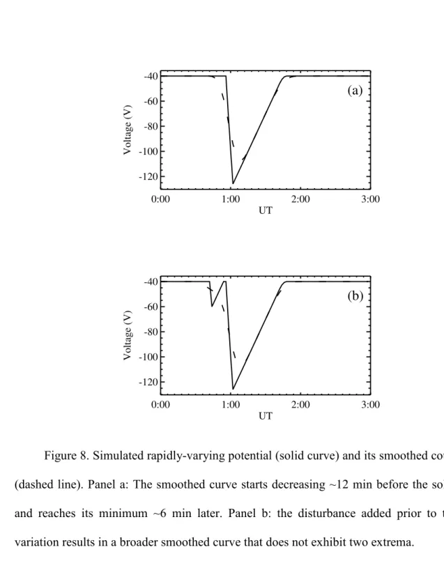
place on a very small time scale. We test this numerical limitation in Figure 8, applying our 5

smoothing method to a simulated signal reproducing the closure voltage of a possible 6

idealised onset (pannel a) and of the same curve preceded by a possible idealised 7

pseudobreakup (pannel b). We assume that the onset develops in ~6 min reaching ~125 kV, 8

after which the voltage then declines at a rate of 2 kV per minute (a reasonable value 9

considering the actual cases) until it returns to the value it had prior to onset. The smearing 10

due to the smoothing procedure results in an error of ~12 min in the start of the negative 11

voltage increase. The minimum voltage (i.e. the maximum magnitude of the reconnection 12

rate) is then reached ~6 min after the extremum of the actual signal, and its value is about 13

15% smaller in absolute value. A time resolution of two minutes was used in this simulation, 14

equal to the time resolution of our datasets. Consequently, when studying rapidly-varying 15

potentials, delays of less than ~16 min are not significant, and the computed voltages will 16

exhibit variations earlier than actually took place. Note as well that a possible pseudobreakup 17

taking place prior to the onset would not be explicitly resolved (panel b), so we cannot 18

determine the detailed time variation of the closure voltage. We conclude that the 19

intensification of the flux closure takes place roughly at the time of the substorm expansion 20

onset, identified at 2038 UT using the IMAGE-FUV images. The maximum closure voltage 21

obtained during the 2038 UT substorm is ~120 kV, but could be as high as ~140 kV, 22

accounting for the bias induced by the smoothing. The maximum is reached at or shortly after 23

substorm onset. The substorm-like event observed starting at 1851 UT was preceded by a 24

series of pseudobreakups, and the computed nightside voltage intensifies 24 min prior to the 25

breakup at 1851 UT. We conclude that flux closure took place significantly prior to the 1851 1

UT onset, resulting in the series of pseudobreakups, consitently with the results of Aikio et al. 2

[1999]. Our method does not allow us to discriminate between a sudden transient increase of 3

the flux closure at the time of the pseudobreakups and a progressive increase ending in the 4

onset. The nightside reconnection rate reaches its maximum magnitude (~100 kV) roughly at 5

the time of onset of this event or shortly after, and could be as high as ~120 kV accounting for 6

the applied smoothing. The substorm starting at 0031 UT (27 December) was preceded by a 7

moderate pseudobreakup at 0004 UT, but no significant intensification in the magnitude of 8

the nightside reconnection rate is indicated between these two events. Nor in this case does 9

the potential drop reach its maximum magnitude around the time of onset, but rather at 0115 10

UT. The IMAGE-FUV images show that several local bright spots appeared during the 11

development of this substorm, suggesting that the mechanism governing its evolution might 12

be more complex than for the other two events discussed above. In Figure 7c, the 0031 UT 13

onset nevertheless appears to be associated with a local extremum of the nightside 14

reconnection rate. The calculated maximum nightside reconnection rate is 116 kV at 0115 UT 15

(possibly as high as ~130 kV for reasons discussed above). 16

The dayside reconnection rate is often estimated using a transfer function based on 17

upstream interplanetary properties. One example of a widely-used function is given by 18

( )

where vSW is the solar wind velocity, BT is the strength of the transverse IMF, and θ is the

20

IMF clock angle with respect to north [Wygant et al., 1983; Liou et al. 1998]. This transfer 21

function has the dimension of an electric field and must thus be multiplied by a characteristic 22

length in order to retrieve a voltage. For southward IMF (θ=180°), this characteristic length L 23

represents the width of the solar wind channel, transverse to the field, which reconnects with 24

the terrestrial field at the magnetopause. Two approaches can then be proposed. As a first 1

order approximation (method 1) one can deduce L from the transfer function computed using 2

the solar wind properties and the open flux determined, for example, from global imaging of 3

the polar region (i.e. using IMAGE-FUV SI12 images) during periods of time when the 4

nightside reconnection rate is expected to be negligible [Milan et al. 2003, 2004; Milan, 5

2004]. We can further refine this approximation (method 2) and compute the ratio between 6

the dayside reconnection rate of Figure 7b and the transfer function of equation 7. The ratio of 7

the dayside reconnection rate (Figures 7b and 9b) and the computed transfer function (Figure 8

9a) is shown in Figure 9c. Reasonable values of the characteristic length are obtained when 9

both the transfer function and the dayside voltage are sufficiently large, giving L ranging 10

between 4 and 15 RE. The characteristic length deduced using the first method is 11 RE for the

11

first substorm of the interval (with onset at 1816 UT), compared with ~10 RE obtained at 1800

12

UT in Figure 9b, and ~3 RE for the second and third (with onsets at 2038 and 0031 UT),

13

compared with ~10 RE at 2000 UT and ~6 RE at 0030 UT. Both methods give results which

14

are not, in essence, different from each other, giving L values of a similar order of magnitude, 15

but method 1 is dependent on the reliability of the assumption of negligible nightside 16

reconnection. This can be critical as we have seen in the present case that the nightside 17

reconnection rate can increase prior to substorm onset, and is generally not less (in absolute 18

value) than ~30 kV. 19

As mentioned in the preceding paragraph, we find that tail reconnection closes magnetic 20

flux at all times, with a typical voltage of ~30 kV during quiet periods. The location of the 21

reconnection site still has to be identified. The quiet time closure voltage is fairly stable, while 22

the voltage of substorm expansion phases exhibits a strong temporal dependence, and during 23

the recovery phase, it progressively returns to a voltage similar to the value prevailing prior to 24

onset. This suggests that the quiet time reconnection rate has not been dramatically modified 25

by the explosive flux closure of the expansion phase. We speculate that this quiet time flux 1

closure takes place in the more distant magnetotail, in accordance e.g. with ISEE-3 2

measurements [Feldman et al., 1984, 1987; Smith et al., 1984; Ho et al., 1994]. 3

4

4.2. 29 December 2000.

5

The IMAGE-FUV instruments also provided continuous coverage of the northern 6

auroral FUV emissions between 0215 and 1045 UT on 29 December 2000. A sample of SI12 7

images corresponding to this interval is presented in a polar view in Figure 10. The 8

corresponding convection velocity and electric equipotentials deduced from the SuperDARN 9

data are presented in Figure 11. A first pseudobreakup is seen at 0241 UT. Two other 10

pseudobreakups occurred at 0320 and 0341 UT, followed by a substorm onset at 0359 UT. A 11

quieter period followed this substorm with variable activity, especially along the polar 12

boundary of the electron aurora, which showed what we identify as a poleward boundary 13

intensification (PBI), similar with those shown by Lyons et al. [2002]. The opened magnetic 14

flux and its time derivative were computed for this interval using the IMAGE-FUV SI12 15

images of the proton aurora and are shown in Figure 12. The shaded regions of Figure 12b 16

indicate southward IMF as observed by the Wind satellite (Figure 13) (the Geotail satellite 17

was not favourably positioned at this time). During this interval Wind was located at GSE (X, 18

Y, Z) ≈ (6, 250, -17) RE, such that an IMF propagation time to Earth of only ~ 1.5 min has

19

been allowed for (an additional small time delay is also added for propagation through the 20

magnetosheath and inner magnetosphere to match the auroral signature). Measurements from 21

both the ACE and Wind satellites indicate a continuous period of southward IMF. Only one 22

transient northward excursion is present in the Wind data (and absent in the ACE data) around 23

0335 UT. As expected for such IMF conditions, the open magnetic flux generally increases in 24

time, except during the substorm expansion phase, and after 0700 UT, apparently due to an 1

intensification of the auroral activity of the PBI. In addition, no trigger based on an IMF Bz

2

sign reversal can be associated with the substorm development, nor can a growth phase period 3

be defined based on IMF Bz reversals. Nevertheless, this period presents an interval of open

4

flux growth followed by an expansion onset that will be discussed in the next paragraphs. 5

The SuperDARN radar network offered very good coverage of the northern polar region 6

during the interval from 0200 to 0450 UT (Figure 11). Later, fewer data are available, but the 7

electric field and potential can still be retrieved. As in the previous example, we thus 8

computed the net rate of change of the amount of open flux as well as the individual ‘dayside’ 9

and ‘nightside’ reconnection rates using both the SuperDARN and IMAGE-FUV SI12 data 10

(Figure 14). Again, the voltage along the moving boundary computed by applying Faraday's 11

law (Figure 14a) and deriving the open flux versus time (Figure 12b) are identical, as 12

expected, so that internal consistency is guaranteed. As in the preceding case, the measured 13

return flow speed was often high during time intervals of increasing Φ, occasionally reaching 14

800 m s-1. After the substorm onset at 0359 UT the return flow remained high, reaching 1000 15

m s-1, despite the decreasing size of the polar cap. After ~0430 UT, the substorm intensity 16

weakened and the competition between nightside and dayside reconnection leads overall to a 17

slowly increasing amount of open magnetic flux. The steep increase of open flux taking place 18

around 0600 UT is characterized locally by a high return flow velocity (more than 1000 m 19

s-1). 20

During and preceding the substorm, the computed nightside voltage shown in Figure 21

14c has a temporal dependence similar in shape to that computed for 27-28 December. Again, 22

the nightside reconnection rate starts to intensify before the substorm onset, but a detailed 23

analysis must be carried out to discriminate between the effect of smoothing and a possible 24

real timing difference. Two pseudobreakups took place during the period preceding the onset 1

at 0359 UT, as in fact often occurs during the growth phase. The computed nightside 2

reconnection rate drops to nearly zero at 0304 UT, about an hour before the substorm onset 3

and 16 min prior to the pseudobreakup at 0320 UT. During this hour, the computed nightside 4

reconnection rate progressively intensifies, more steeply during the ten minutes preceding the 5

onset. We consider that this increase leading up to the onset is real (significantly longer than 6

~16 min), resulting in the observed pseudobreakups. However, we cannot determine whether 7

the nightside flux closure increases progressively, or if it suddenly increased at the time of the 8

observed pseudobreakups. It must be noted that the GOES-8 satellite, ideally located near the 9

midnight sector at the time of the pseudobreakups and onset, recorded a variation of the Bx

10

component of the magnetospheric field suggesting a dipolarization (not shown). Also the AE 11

and AL indices were disturbed prior to what we identify as the onset. Examination of 12

magnetograms from the CANOPUS-CARISMA and IMAGE (for International Monitor for 13

Auroral Geomagnetic Effects, not to be confused with the IMAGE satellite) networks (not 14

shown) would rather indicate that the brightening recorded at 0341 can be considered as an 15

intense pseudobreakup, despite similarities with substorm onsets. Indeed, the spot of the 16

pseudobreakup is still bright at the time of the onset thus mixing both signatures. This 17

suggests that both features could be intimately linked together, so that the possibility of a 18

multiple onset scenario cannot be categorically ruled out. Nevertheless, the thickening of the 19

oval characteristic of an expansion phase is observed following the brightening of 0359 UT, 20

and the open flux keeps increasing until that time, indicating that the end of the growth phase 21

is taking place. This leads us to the conclusion that the substorm onset is actually the 22

brightening observed at 0359 UT. Several authors [Aikio et al., 1999, Akasofu, 1964, 23

Koskinen et al., 1993] considered that pseudobreakups and substorm onsets are not of 24

fundamentally different physical nature, and only differ in magnitude and in the conditions 25

met at the time of their development. From that standpoint, we can expect to record 1

disturbances with groundbased magnetometers in response to a pseudobreakup, revealing a 2

modification of the current systems, and it seems natural as well to find that both 3

pseudobreakups and substorms are associated with flux closure. Along the same lines, a 4

dipolarization cannot be ruled out during a pseudobreakup, since it is a natural signature of 5

magnetic reconnection in the tail. The computed nightside reconnection rate reaches its 6

maximum magnitude (140 kV) about ten minutes after onset and then returns to quiet values 7

varying around ~40 kV. The maximum rate of flux closure is obtained roughly at the time of 8

the onset or shortly after. This extreme value could be as high as ~160 kV, taking the 9

smoothing into account. The onset of the substorm presented in this section was preceded by 10

an interval of intense dayside reconnection (between 120 and 130 kV, Figure 14b) feeding the 11

magnetosphere with open magnetic flux. This interval of intense flux opening sets up the 12

necessary conditions to produce the development of a substorm (i.e. accumulation of open 13

flux) and is thus the growth phase of the substorm considered, despite the absence of a switch 14

in sense of IMF Bz. Figure 15 presents WIC images obtained after 06:30 UT, which show the

15

PBI at different times between 0630 and 1000 UT . Note that the oscillations present in the 16

nightside voltage prior to 0600 UT appear to be driven by a roughly periodic variation of the 17

dayside reconnection voltage (with some phase displacement between these two curves, as 18

naturally expected). The nightside reconnection voltage progressively increases after 0630 19

UT, and finally dominates the dayside flux opening voltage leading to a global contraction of 20

the polar cap. This increase of the flux closure rate reaches 68 kV and departs from the 21

sudden intensification of the nightside voltage associated with an expansion phase onset. A 22

brightening of the PBI is also seen, and the morphology of the oval evolves to a shape similar 23

to expansion phase conditions (figure 15 after 0800 UT). This interval suggests that an 24

intensification of the flux closure rate of the magnetosphere can activate the auroral 25

precipitation in the PBI, and thus suggests a direct relation between PBI auroral structures and 1

flux closure in the magnetotail. 2

Finally, we calculated the characteristic solar wind scale length for reconnection L using 3

both method 1 (not shown), and method 2 (Figure 16) discussed previously. As the IMF was 4

always southward during the interval considered, the transfer function is always quite large 5

(Figure 16a), and the dayside voltage is also nearly always high (Figure 16b). It should be 6

noted that the dayside voltage reached a maximum value of 130 kV around 0340 UT, roughly 7

at the time the transfer function reached a local minimum, indicating that care must be taken 8

when using a transfer function to evaluate the dayside voltage. At this time, we obtain L ~18 9

RE. The characteristic solar wind scale length calculated here indicates strong temporal

10

variability, but remains of a reasonable order of magnitude. These values can be compared 11

with a length obtained with method 1 of ~8 RE between 0220 and 0310 UT, and ~3 RE

12

between 0310 and 1040 UT. 13

4.3 Other cases

14

We studied four other time intervals of ~9 h each close to winter solstice 2000 (0335 to 15

1215 UT on 23 December, 1800 UT on 23 December to 0315 UT on 24 December, 1215 to 16

2225 UT on 25 December, and 0300 to 1200 UT on 26 December), and reached similar 17

conclusions. Flux closure can take place prior to substorm onset resulting in pseudobreakups 18

during the growth phase. Maximum flux closure is generally reached roughly at the time of 19

the substorm onset. The flux closure rate slowly decreases (in absolute value) after the onset, 20

back to ~30 to ~40 kV. However, some substorms were found to depart from this simple 21

picture, especially during periods of prolonged intense nightside reconnection rates (such as 22

23 and 24 December 2000 for example), making the substorm analysis more complicated, 23

especially the optical identification of the substorm onset. The maximum rate of flux closure 1

is then variable, but generally above 100 kV. 2

3

5. Discussion

4

Several sources of uncertainties can complicate the calculation of the amount of open 5

flux and the reconnection rates determined by combining IMAGE-FUV SI12 images of the 6

proton aurora and SuperDARN measurements of the convection flow. The first source is the 7

temporal smoothing that must be applied when determining the velocity of the open/closed 8

field line boundary. As already discussed in the preceding sections, this smoothing results in a 9

smearing of short time scale features. As a result, the increase in the computed nightside 10

reconnection rate is seen ~12 to 14 min prior to onset, and a temporal difference less than ~16 11

min is probably not significant. However, when substorm onsets are preceded by 12

pseudobreakups, some significant flux closure is found prior to onset though its detailed time 13

dependence (a transient or more gradual variation) cannot be determined. A second side effect 14

of the smoothing is an underestimate (in absolute value) of the maximum nightside voltage. 15

A second source of uncertainty lies in the least squares fit used to represent the 16

open/closed boundary with a Fourier series. This fitted series cannot always reproduce the 17

details of the boundary. On the other hand, it spatially smooths the boundary determined from 18

the SI12 images. The fitted Fourier series is smooth in essence and filters out the noise around 19

the boundary. However, on some occasions, this fitted boundary departs locally from the 20

actual boundary due to the oscillation of the terms in the Fourier series. The temporal 21

smoothing partly corrects for this drawback by averaging these unrealistic oscillations. In 22

addition, the Fourier series can be extrapolated when a part of the proton oval is not bright 1

enough to be detected using SI12. 2

We also note that our identification of the open/closed field boundary does not include a 3

particular treatment of the cusp. As a bright feature, the cusp is not distinguished from the 4

auroral oval. However, the cusp is threaded by open field lines whereas the auroral oval is 5

threaded by closed field lines. This leads to an underestimate of the open magnetic flux by a 6

few percent, which is not likely to be of major significance. The effect on the computed 7

voltages has already been discussed in section 3. 8

Another source of error is associated with the electric field determined using the 9

SuperDARN data. The location of the SuperDARN radars does not allow a complete 10

coverage of the northern region. Consequently, when the electric potential is determined using 11

a least squares fit (constrained by a model), it generally includes some extrapolation, which 12

can sometimes depart from the actual potential. In addition, the appearance or disapearance of 13

radar echoes in the polar cap can occur abruptly, modifying the fitted electric field. This can 14

lead to artificial variations of the reconnection voltages determined. Nevertheless, the 15

smoothing versus time that is applied should reduce the effect of transient unrealistic 16

variations on the computed voltages. However, the bulk of the total electric field results from 17

the motion of the open/closed boundary, especially during substorms, or in other words the 18

boundary moves first and some time later convection gradually redistributes the flux to an 19

equilibrium position [Cowley and Lockwood, 1992]. 20

One can also question the relation between the electric field and voltage computed in 21

the ionosphere and the electric field and voltage at the reconnection site: some potential drop 22

might take place between the ionosphere and the reconnection site. It is however often 23

assumed as a first approximation that magnetic field lines are electric equipotentials, because 24