Relationship between sedimentary features and permeability
at different scales in the Brussels Sands
Mathias POSSEMIERS1, Marijke HUYSMANS1, Luk PEETERS1,2, Okke BATELAAN1,3 & Alain DASSARGUES1,4 1 KU Leuven, Applied Geology and Mineralogy, Department of Earth and Environmental Sciences, Celestijnenlaan 200 E, 3001 Heverlee,
Belgium. E-mail: mathias.possemiers@ees.kuleuven.be.
2 CSIRO Land and Water, Waite Campus, Waite Road Urrbrae, Australia.
3 Vrije Universiteit Brussel, Department of Hydrology and Hydraulic Engineering, Pleinlaan 2, 1050 Brussels, Belgium.
4 Université de Liège, Hydrogeology and Environmental Geology, Department of Architecture, Geology, Environment and Civil
Engineering (ArGEnCo), B.52/3 Sart-Tilman, 4000 Liège, Belgium.
ABSTRACT. The Brussels Sands display a complex three-dimensional subsurface architecture. This sedimentological heterogeneity induces a highly heterogeneous spatial distribution of hydrogeological parameters at different scales and may consequently influence subsurface fluid flow and solute migration. This study aims at characterizing spatial variability of permeability at different scales in the Brussels Sands. Firstly, a literature review on the permeability distribution of the Brussels Sands was performed. Secondly, a field campaign was carried out consisting of field observations of the small-scale sedimentary structures and in situ measurements of air permeability. A total of 6550 cm-scale air permeability measurements were carried out in situ in three Brussels Sands quarries in the central part of Belgium: Bierbeek, Mont-Saint-Guibert and Chaumont-Gistoux. On the large basin scale, substantial differences in permeability are observed. A literature data analysis shows that there is no clear correlation between hydraulic conductivity and sedimentary facies. At the small scale, results show that permeability heterogeneity and anisotropy are strongly influenced by sedimentary heterogeneity in all three quarries. Clay-rich sedimentary features such as bottomsets and distinct mud drapes exhibit a different statistical and geostatistical permeability distribution compared to the cross-bedded lithofacies, where the permeability anisotropy is dominated by the foreset lamination orientation.
KEYWORDS: Geological heterogeneity; Sedimentary structures; Air permeability; Hydraulic conductivity; Geostatistics
1. Introduction
The Brussels Formation is an early Middle Eocene shallow marine sand deposit in central Belgium and constitutes a major groundwater resource in the region. The Brussels Sands occur in a 40 km wide SSW-NNE oriented zone in central Belgium (Fig. 1). These sands fill an approximately 120 km long and 40 km wide embayment which ended in the north of the Province of Antwerp in the North Sea. The base of the sands is characterised by two central major SSW-NNE trending troughs and several minor troughs with the same orientation. The Brussels Sands consist of unconsolidated quartz sands with variable percentages of feldspar, silex, glauconite, lime and heavy minerals (Gulinck & Hacquaert, 1954). Three main facies types can be distinguished: a coarse cross-bedded facies, a bioturbated facies and a massive facies (Houthuys, 1990). The spatial occurrence of the different facies types displays strong lateral and vertical variations. The Brussels Sands Formation is therefore characterised by a complex three-dimensional subsurface architecture of sedimentary structures and facies types. Three different hierarchical levels of geological heterogeneity can be identified in the Brussels Sands similarly to Van de Graaff & Ealey (1989): (1) large-scale heterogeneity (≈ 5-50 km scale) related to the geometry and dimensions of the
sand body; (2) meso-scale heterogeneity (≈ 10 m to 5 km scale) related to spatial trends in grain size and permeability within the sand body due to vertical and lateral facies changes; and (3) small-scale heterogeneity (≈ 1 mm to 10 m scale) mainly related to cross-bedding. More details about the sedimentary structures and depositional environment of the Brussels Sands can be found in Houthuys (1990) and Houthuys (2011).
The complex sedimentological heterogeneity of the Brussels Sands results in a highly heterogeneous spatial distribution of permeability at different scales. Such a heterogeneous permeability distribution may affect fluid flow and solute migration significantly (Koltermann & Gorelick, 1996; Klingbeil et al., 1999). Several authors found that preferential flow paths on centimetre to decimetre scale have a significant impact on the spread of pollutants (Zheng & Gorelick, 2003; Huysmans & Dassargues, 2009). Ignoring the heterogeneity therefore can have profound implications for the remediation of contaminated groundwater. Neglecting or incomplete characterization of a complex permeability distribution in hydrogeological models can lead to erroneous predictions in direction and speed of contaminant transport (Huysmans & Dassargues, 2009). Permeability heterogeneity should therefore be understood and incorporated into groundwater and transport models.
This study aims at giving an overview of large-scale and small-scale permeability heterogeneity in the Brussels Sands and at validating the conclusions of Huysmans et al. (2008) in other Brussels Sands quarries. The relation between the spatial variability of permeability and geological heterogeneity is investigated at different scales. This approach is similar to several studies that map the spatial distribution of permeability in detail and identify the relationship between sedimentary structures and permeability (Anderson, 1989; Dreyer et al., 1990; Davis et al., 1993; Fogg et al. 1998; Klingbeil et al., 1999; Morton et al., 2002; Heinz et al., 2003; Van den Berg & de Vries, 2003; Mikes, 2006; Tipping et al., 2006). Firstly, a literature review on permeability of the Brussels Sands is performed. Secondly, a field campaign consisting of field observations of the sedimentary structures and in situ measurements of air permeability in three Brussels Sands quarries is described.
2. Permeability of the Brussels Sands: a review
Permeability (or intrinsic permeability) and hydraulic conductivity are measures of the resistance to fluid flow through Figure 1. Map of Belgium showing Brussels Sands outcrop and subcrop
area (shaded part) and the location of the Bierbeek quarry, the Chaumont-Gistoux quarry and the Mont-Saint-Guibert quarry (modified after Houthuys, 1990).
R b s 157
a porous medium under a specified hydraulic gradient. Intrinsic permeability k depends on the properties of the medium alone. Hydraulic conductivity K depends both on the properties of the solid medium and on the density and viscosity of the fluid. Hydraulic conductivity is defined as the product of the intrinsic permeability and the specific weight of water, divided by the dynamic viscosity: Formule 1 g k K Formule 3 11 . 14 ) log( 27 . 1 ) log(K ka Formule 4 93 . 13 ) log( 22 . 1 ) log(K ka Formule 5 ) ) (( 2 0 2 2 2 1 1 1 a G P P Q P k (1)
where K is hydraulic conductivity (ms-1), k is intrinsic permeability (m²), ρ is the density of the fluid (kgm-3), g is the acceleration of gravity (ms-2) and μ is dynamic viscosity of the fluid (kgm-1s-1). A widely used unit for intrinsic permeability k is the darcy (d):
2 13 2 3 10 87 . 9 / 1 1 / 1 1 ) ( 1 m cm atm cm s cm cP d darcy = = − m r g k K = 11 . 14 ) log( 27 . 1 ) log(K = ka + 93 . 13 ) log( 22 . 1 ) log(K = ka + ) ) (( 2 0 2 2 2 1 1 1 a G P P Q P k − = m 2 ) , ( ( ) ) ( 2 1 ) (h = Nh
∑
ijhij=h vi−vj γ (2)where cP is centipoise (unit for viscosity) and atm is atmosphere (unit for pressure) (Fetter, 2001). Several authors have also established empirical relationships between air permeability (ka) and hydraulic conductivity (K). Ideally, the intrinsic (saturated
water) permeability (k) and air permeability (ka) should be the same, and k can be replaced by ka in equation 1. In reality however, totally dry conditions are hard to obtain, and might cause breakdown of the sediment structure. Furthermore, water as a polar fluid tends to interact with the soil components and air at atmospheric pressure does not act as a true fluid continuum in the soil (Iversen et al., 2003). Jalbert & Dane (2003) found that in sandy loam samples, permeability values obtained with air were larger than those obtained with water. On average, the ratio of the air permeability/hydraulic conductivity was 1.43. It can be physically explained by the lower affinity of air, compared to water, for the solid matrix. Loll et al. (1999) derived the following log-log linear relationship between air permeability and saturated hydraulic conductivity based on data from a total of 1614 soil samples: Formule 1 g k K Formule 3 11 . 14 ) log( 27 . 1 ) log(K ka Formule 4 93 . 13 ) log( 22 . 1 ) log(K ka Formule 5 ) ) (( 2 0 2 2 2 1 1 1 a G P P Q P k (3)
where K and ka are in units of (md-1) and (m²) respectively. Iversen et al. (2003) found a very similar relationship between air permeability and saturated hydraulic conductivity based on 62 soil samples:
Formule 1 g k K Formule 3 11 . 14 ) log( 27 . 1 ) log(K ka Formule 4 93 . 13 ) log( 22 . 1 ) log(K ka Formule 5 ) ) (( 2 0 2 2 2 1 1 1 a G P P Q P k (4)
Figure 2. Spatial variability of
the hydraulic conductivity in the Brussels Formation based on several literature references.
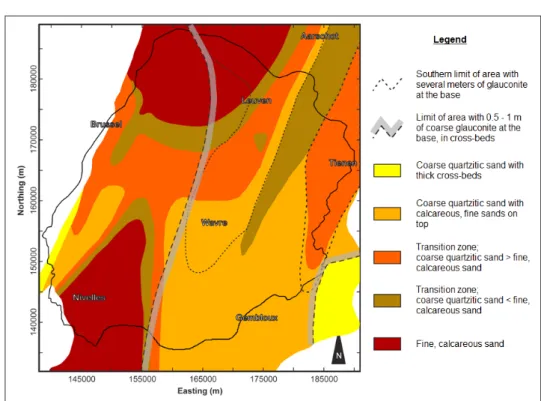
Figure 3. Brussels Sands facies
distribution (modified after Houthuys, 1990).
As permeability and hydraulic conductivity are closely related properties, an overview of both properties of the Brussels Sands is given.
Many papers, technical reports and hydrogeological maps report hydraulic conductivity values for the Brussels Sands, usually obtained from single-well tests and pumping tests (Bronders & De Smedt, 1991; Chabot, 1996; Ruthy & Dassargues, 2001, 2002; Haecon, 2007; VMW internal technical reports). The overall hydraulic conductivity in the Brussels Sands is high, generally above 2 10-5 m/s, and very variable. Values between 2.5 10-5 m/s and 7.3 10-4 m/s are reported. Fig. 2 shows the spatial variability of hydraulic conductivity values in the Brussels Formation (based on values from Bronders & De Smedt, 1991; Ruthy & Dassargues, 2001, 2002; VMW internal technical
reports). The coarse facies, as mapped by Houthuys (1990), in the Brussels Sands is expected to have a higher conductivity. This is observed locally using pumping tests (VMW, internal technical reports) but a correlation between the spatial variability of hydraulic conductivity and the facies map of Houthuys (1990) is not prominent (Figs 3 and 4). Lateral facies changes are so numerous and unexpected that a facies map is difficult to establish and can only bring a preliminary grouping in facies associations (Houthuys, 1990, 2011). This inaccuracy of the facies map, differences in layer thickness and presence of alluvial gravels as well as the reliability of the pumping and single-well tests can hamper a clear relation. It indicates that the relation between hydraulic conductivity and sedimentary facies is a complex relation and that the relation between hydraulic conductivity and grain size is not straightforward.
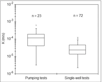
Bronders (1989) observes systematically lower K-values obtained from single-well tests compared to data from pumping tests. Boxplots from the K-values for the Brussels Formation confirm this observation (Fig. 5). The mean of K-values of single-well tests (Bronders & De Smedt, 1991) and pumping tests (Bronders & De Smedt, 1991; Ruthy & Dassargues, 2001, 2002; VMW, internal technical reports) are 3.08 10-5 m/s and 1.45 10-4 m/s respectively, the standard deviations are 2.34 10-5 m/s and 1.44 10-4 m/s respectively. The observed difference between K-values from pumping tests and single-well tests can be partly attributed to the quality of data and the installation of the piezometers wherein the single-well tests were performed. Clogging of piezometers can for instance result in lower K-values from a well test. Additionally, a single-well test only provides information on the hydraulic conductivity in the immediate vicinity of the well. In the single-well tests the piezometer is pumped at a constant pumping rate until groundwater head stabilizes. From the difference between initial head and stabilized head during pumping, hydraulic conductivity of an unconfined aquifer can be calculated (Bronders, 1989). Pumping tests on the other hand represent larger volumes of the aquifer, because here the aquifer response is observed in observation wells on a certain distance of the pumping well. K-values from single-well tests can therefore be more variable due to local heterogeneity. Another reason is that pumping wells generally are developed to increase the productivity of the wells. It has to be noted however that the difference between single-well and pumping tests in the Brussels Formation at least partly can be attributed to the location of the pumping wells. Pumping wells for drinking water production are mainly located in alluvial valleys where the Brussels Aquifer is directly in contact with the Pleistocene gravels and coarse sands (e.g. Heverlee Cadol, Egenhoven, Abdij van ‘t Park) or in the coarse facies of the Brussels Sands (e.g. Winksele Kastanjebos, Herent Bijlok).
Figure 4. Boxplots of hydraulic conductivity (K); A) Per sedimentary
facies: 1) coarse quartzitic sand with calcareous, fine sands on top, 2) transition zone: coarse quartzitic sand > fine calcareous sand, 3) transition zone: coarse quartzitic sand < fine calcareous sand, 4) fine calcareous sand; B) Per glauconite facies: 1) no or limited glauconite at base, 2) 0.5 to 1 m coarse glauconite at base, in cross-beds, 3) several meters coarse glauconite at base, in cross-beds. The ends of the whiskers are set at 1.5 IQR above the third quartile (Q3) and 1.5 IQR below the first quartile (Q1).
Figure 5. Boxplots of K-values from pumping tests and single-well tests.
The ends of the whiskers are set at 1.5 IQR above the third quartile (Q3) and 1.5 IQR below the first quartile (Q1). (Data from Bronders & De Smedt, 1991; Ruthy & Dassargues, 2001, 2002; VMW, internal technical reports).
R b s 159
Pumping tests at these locations, selected for their production capacities, will therefore yield higher hydraulic conductivity values.
On a small scale, sedimentary structures may strongly influence hydraulic conductivity. In Huysmans et al. (2008) the sedimentary heterogeneity and the spatial distribution of permeability in the Brussels Sands on a small scale is mapped for the Bierbeek sand quarry (Lambert-72 coordinates: x: 176250, y: 169900). A large number of cm-scale air permeability measurements was performed. The results indicate that clay-rich sedimentary features such as bottomsets and muddrapes have a distinctly different hydraulic conductivity distribution compared to other lithofacies in the cross-bedded sands. Since all measurements of Huysmans et al. (2008) were performed in only one Brussels Sands quarry, it is unclear whether these results can be extrapolated to other locations or facies types in the Brussels Sands.
The present study aims at validating the conclusions of Huysmans et al. (2008) in other Brussels Sands quarries and at characterizing the spatial variability of permeability at different scales in the Brussels Sands. Therefore additional air permeability measurements were carried out in two other Brussels Sands quarries: Mont-Saint-Guibert (x: 168350, y: 149050) and Chaumont-Gistoux (x: 174500, y: 150800) (Fig. 1). For each of the three quarries the relationship between small-scale sedimentary structures and the permeability was investigated. Permeability differences between the different quarries were also investigated and interpreted.
3. Methodology
3.1. Air permeability measurements
Air permeameters have been used in a wide variety of laboratory and field applications where localized small-scale measurements are needed to characterize the spatial distribution of permeability (e.g., Goggin et al., 1988a; Dreyer et al., 1990; Jacobsen & Rendall, 1991; Hartkamp et al., 1993; Tidwell & Wilson, 1999; Castle et al., 2004). In situ permeameters can reveal several orders of magnitude of permeability contrast missed by conventional core plug measurements (Goggin et al., 1988b; Halvorsen & Hurst, 1990). A device for obtaining small-scale air permeability measurements was first described by Dykstra & Parsons (1950). Later, Eijpe & Weber (1971) constructed a minipermeameter for measuring the permeability of rock and unconsolidated sands. A probe permeameter is basically an annulus through which gas (nitrogen or air) can be released into porous media. Gas flow rate and gas pressure are monitored and can be transformed into gas permeability by empirically derived relationships or by use of an analytical equation, such as the modified form of Darcy’s law including a geometrical factor depending on tip seal size proposed by Goggin et al. (1988a, b):
Formule 1 g k K Formule 3 11 . 14 ) log( 27 . 1 ) log(K ka Formule 4 93 . 13 ) log( 22 . 1 ) log(K ka Formule 5 ) ) (( 2 0 2 2 2 1 1 1 a G P P Q P k (5)
where k is permeability, μ is the gas viscosity at atmospheric pressure, P1 is injection pressure, P2 is outflow pressure, Q1 is the volumetric rate at injection pressure P1, G0 is a dimensionless geometric factor and a is the radius of the seal area. The depth of investigation of a minipermeameter is approximately four times the internal radius of the tip seal according to Goggin et al. (1988b). In an isotropic porous medium, the measurement volume corresponds to a hemispherical shaped volume of rock with a radius of approximately four times the internal radius of the tip seal. Jensen et al. (1994) found that probe permeameter measurements are even more localized with a depth of investigation of the order of only two probe inner radii.
In this research project air permeability was measured using a portable permeameter, the TinyPerm II distributed by New England Research. Permeability measurements were taken by pressing the device against the quarry face and depressing the plunger to withdraw air from the porous medium. Leakage between the annulus and the rock is avoided by a compressible, impermeable rubber tip. The inner tip radius is 4.5 mm and the outer tip radius is 12 mm. According to the equations of Goggin
et al. (1988b) and Jensen et al. (1994), this means that the depth of investigation of the TinyPerm is between 9 and 18 mm. The measurement volume is in this case a hemispherical shaped volume with a radius between 9 and 18 mm. A micro-controller unit computes the response function of the sample-instrument system using the measured air volume and vacuum pulse. This response function is related to the air permeability of the sample by a calibration curve (Huysmans et al., 2008).
A total of 6550 cm-scale air permeability measurements were carried out in-situ on different faces in three Brussels Sands quarries. In Bierbeek, Mont-Saint-Guibert and Chaumont-Gistoux respectively 2750, 3000 and 800 air permeability measurements were carried out divided over several rectangular grids. The measurement spacing was adjusted to the lamina thickness so that the vertical and horizontal spacing is between 2 and 5 cm.
The permeability measurements in the Bierbeek quarry are performed in facies X (Houthuys, 2011). This facies is characterised by thick cross-beds, often thicker than 1 meter. The sand is very coarse and there are few bioturbations. Furthermore, a significant portion of the sand is composed of glauconite (15-20%) and the muddrapes are very continuous. The permeability measurements in the Mont-Saint-Guibert quarry were like the ones in Bierbeek carried out in facies X (Houthuys, 2011). In Mont-Saint-Guibert however no or little glauconite is found and the muddrapes are less continuous. In Chaumont-Gistoux the permeability measurements were performed in facies Xb and Bx (Houthuys, 2011). These two facies merge into one another, the Xb facies consists of cross-beds composed of sand with average grain size in which many bioturbations occur, while facies Bx is very strongly bioturbated, but in which the thin cross-beds are still recognisable.
3.2. Geostatistical analysis
To detect trends and patterns in the permeability distribution, a statistical and geostatistical analysis was carried out. Univariate statistical analysis allowed summarizing permeability measurements and comparing the average permeabilities measured in the different quarries. The geostatistical analysis was developed to describe the spatial relation between the small-scale sedimentary structures and permeability. In the geostatistical analysis, semivariograms and semivariogram maps of measured permeability were constructed. The semivariogram, or simply variogram
g
(h), is defined as half the average squared difference between the values of two random data points vi and vj forming a pair and which are separated by a certain distance, lag vector h (Isaaks & Srivastava, 1989):2 13 2 3 10 87 . 9 / 1 1 / 1 1 ) ( 1 m cm atm cm s cm cP d darcy = = − m r g k K = 11 . 14 ) log( 27 . 1 ) log(K = ka + 93 . 13 ) log( 22 . 1 ) log(K = ka + ) ) (( 2 0 2 2 2 1 1 1 a G P P Q P k − = m 2 ) , ( ( ) ) ( 2 1 ) (h = Nh
∑
ijhij=h vi−vj γ (6)where N(h) is the number of pairs. The variogram describes the variance as a function of spatial variation. Low variogram values indicate a high degree of correlation between the data points separated by a lag vector, while high variogram values indicate a low degree of correlation. Spatial variability is often anisotropic so variograms are different when calculated in different directions (Isaaks & Srivastava, 1989). A variogram map allows quantifying the spatial correlation of permeability in different directions by contouring variogram values. In variogram maps the largest continuity corresponds to the direction where the mean squared difference between the measuring points is smallest. All experimental variograms were modelled using an indicative goodness-of-fit criterion, which is a weighted least squares measure of the agreement between the experimental and model variogram. The shape of the variograms suggested fitting by a spherical model. A spherical variogram is defined by three variogram parameters: nugget, sill and range. The nugget value reflects the very small-scale variability. The sill value reflects the total variability within the data set. The variogram range is a measure for the distance until which sample values are spatially correlated.
3.3. Grain size analysis
In each quarry, two representative sand samples were taken for grain size analysis. Grain size analysis was performed to quantify the grain size differences between the quarries. Grain size was
analysed in the laboratory using two different techniques: Low Angle Laser Light Scattering and dry sieving.
In Low Angle Laser Light Scattering (LALLS), the laser light is scattered by the particles. The size of the particles will determine the scattering angle and intensity. The grain size that can be measured in the used laser diffraction system (Malvern Mastersizer Type S Long Bed Version 2.15) is between 0.5 and 900 µm. This method is especially sensitive to small differences in grain size. It is a very fast method that allows analysing particles smaller than 2 μm and both sand and fine material can be measured using a single method (McCave and Syvitski, 1991; Malvern Instruments Ltd., 2011).
The sieving was conducted in dry conditions in a sieve column with 8 sieves with different mesh sizes. The eight used sieves had mesh sizes of 45, 63, 90, 125, 180, 250, 355 and 500 μm. The sieve column with the sample was shaken on a Retsch AS 200 sieve apparatus during 10 minutes. Finally, the fractions that remained on the different sieves were weighed.
These two methods for measuring grain size distribution were chosen for their different approach. The Low Angle Laser Light Scattering gives the grain size distribution in volume percentage whereas the dry sieving results in a mass percentage. Moreover the samples were measured without pre-treatment: in the laser the grains were disaggregated due to the ultrasonics in the water reservoir of the sample dispenser, whereas in the dry sieving the samples were sieved without any disaggregation (dry conditions). Hence, the results obtained by these two techniques can be different which enhances the interpretation of the grain size distributions.
4. Results and discussion
4.1. Large-scale spatial variation of permeability
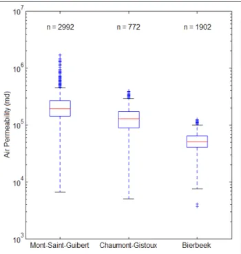
Average air permeabilities are 58,700 md in the Bierbeek quarry, 135,730 md in the Chaumont-Gistoux quarry and 223,871 md in the Mont-Saint-Guibert quarry (Fig. 6). Using the formula of Loll (1999), this corresponds to average hydraulic conductivities of 1.49 10-4 m/s in the Bierbeek quarry, 4.31 10-4 m/s in the Chaumont-Gistoux quarry and 8.14 10-4 m/s in the Mont-Saint-Guibert quarry. These values lie within the hydraulic conductivity range obtained by pumping tests and single-well tests. Considerable differences in permeability are observed between the three different quarries. To explain these differences in permeability, hydraulic conductivity in the three quarries is compared to grain size. The Laser analysis (Fig. 7) shows that the grain size of the samples taken in Mont-Saint-Guibert is larger than in the quarries in Bierbeek and Chaumont-Gistoux. The samples from Chaumont-Gistoux have a slightly smaller grain size than the samples from Bierbeek. Table 1 also shows that the D10 and D50 values of the samples from Chaumont-Gistoux are Figure 6. Boxplots of air permeabilities (md) measured in the
Mont-Saint-Guibert, Chaumont-Gistoux and Bierbeek quarries. The ends of the whiskers are set at 1.5 IQR above the third quartile (Q3) and 1.5 IQR below the first quartile (Q1).
Figure 7. Grain size distributions
for the Mont-Saint-Guibert, Chaumont-Gistoux and Bierbeek quarry using Low Angle Laser Light Scattering (2 samples (A and B) per quarry).
D
10(µm)
D
50(µm)
Mont-Saint-Guibert A
227
421
Mont-Saint-Guibert B
106
405
Chaumont-Gistoux A
21
274
Chaumont-Gistoux B
39
301
Bierbeek A
149
331
Bierbeek B
152
332
Table 1: D10 and D50 values determined using Low Angle Laser Light
R b s 161
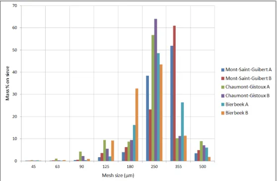
smaller than those from Bierbeek. Striking is the large amount of very small particles in Chaumont-Gistoux (see D10 value), where these aren’t present in the dry sieving (Fig. 8). This can be explained by the large amount of iron oxides in the Chaumont-Gistoux samples. In the laser analysis they came loose from the larger particles by disaggregation in the water reservoir, where they stayed attached to the larger particles in the dry sieving. The sieve analysis (Fig. 8) shows that for the samples from Mont-Saint-Guibert the largest fraction (mass percent) is found on the 355 µm sieve, while the largest fraction for Bierbeek and Chaumont-Gistoux is found on the 250 µm sieve. For the samples taken in Bierbeek (especially Bierbeek B) also a large mass fraction is found on the 180 µm sieve.
The higher average permeability in Mont-Saint-Guibert can be explained by the larger average grain size. For the other two quarries the grain size results from LALLS and dry sieving contradict each other. Grain size certainly plays an important role in the permeability of the investigated sands, but also other properties of the sands are affecting permeability such as grain shape and sorting. Furthermore, the continuity of the mud drapes may play a role. The lower permeability in the Bierbeek quarry can possibly be explained partially by this factor (Houthuys, pers. comm.).
4.2. Small-scale spatial variation of permeability
In Fig. 9 there is made a split of the air permeabilities in function of sedimentary structure (foresets, bottomsets and muddrapes)
for each quarry separately. When the Mont-Saint-Guibert quarry is considered there is a clear difference between the air permeabilities of the foresets, bottomsets and muddrapes. Foresets have higher air permeabilities than bottomsets and bottomsets have higher air permeabilities than muddrapes. But when the same visualization is made for Chaumont-Gistoux and Bierbeek there is not such a relation. The reason for this anomaly is a less clear boundary between the bottomsets, foresets and muddrapes in the Chaumont-Gistoux and Bierbeek quarries (Fig. 10) in comparison with the Mont-Saint-Guibert quarry (Fig. 11).
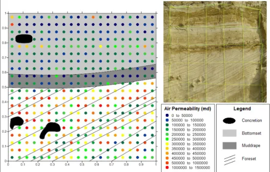
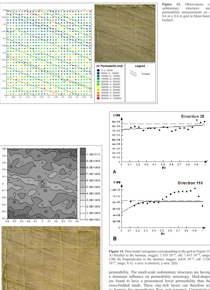
In some measured grids there is clearly a direct visual link between sedimentary structure and permeability. Fig. 11 shows the results of observations of sedimentary structures and the permeability measurements on a 1 m x 1 m grid in Mont-Saint-Guibert. On this grid 400 air permeability measurements were performed with a vertical and horizontal spacing of 5 cm. Different sedimentary structures are present such as a foreset, bottomset and mud-drapes. The highest permeabilities occur in the foreset while the lowest permeabilities occur in the muddrapes. When there is not a distinct lithology contrast, the visual link between sedimentary structure and permeability is not that clear, this is shown in a 0.6 m x 0.6 m grid in Mont-Saint-Guibert (Fig. 12). On this grid 900 air permeability measurements were made at a 2 cm spacing. This grid is entirely located in the foreset.
All the 6550 permeability measurements made in Bierbeek (Huysmans et al., 2008), Mont-Saint-Guibert and Figure 8. Grain size fractions
on sieves for the Mont-Saint-Guibert, Chaumont-Gistoux and Bierbeek quarry (2 samples (A and B) per quarry).
Figure 9. Boxplots of
the air permeability per sedimentary structure and per quarry. The ends of the whiskers are set at 1.5 IQR above the third quartile (Q3) and 1.5 IQR below the first quartile (Q1).
Chaumont-Gistoux were analysed geostatistically. Variograms and variogram maps were calculated for each measured grid. Fig. 13 shows a variogram map with its corresponding grid. The direction where the mean squared difference between the measuring points is smallest, or the direction of largest continuity, is very clear in this variogram map. Although the direction of the maximum continuity in permeability and the slope of the laminae may vary slightly, we can conclude from the calculated variogram maps that the largest continuity is in the direction of the foreset laminae. Therefore, the directional variograms are calculated both in the direction parallel to the laminae and in the direction perpendicular to the laminae. The calculated directional variograms in this study all show a clear anisotropy, the directional variograms parallel to the laminae all show a larger range than the directional variograms perpendicular to the laminae. This means that the permeability has a larger continuity in the direction parallel to the laminae than in the direction perpendicular to the laminae. The directional variograms corresponding to the variogram map in Fig. 13 are shown in Fig. 14.
5. Conclusion
In this study, the spatial variability of permeability was reviewed and characterized at different scales in the Brussels Sands. At the large scale there is a large heterogeneity in hydraulic conductivity which is reflected in the literature values from pumping tests and single-well tests. At this large scale there is no apparent correlation between the spatial variability of hydraulic conductivity and the facies distribution of Houthuys (1990). The link between conductivity data and the facies map is difficult to establish since the lateral facies changes are so numerous and unexpected that the facies map can only bring a preliminary grouping in facies associations. Moreover, the relation between hydraulic conductivity and sedimentary facies is very complex. The results also show that there are large differences in permeability between the different quarries. These differences in permeability between the different quarries can only be partly explained by differences in grain size. Other controlling factors can be grain shape, sorting and arrangement of grains.
When the Mont-Saint-Guibert quarry is considered there is a clear difference between the air permeabilities of the foresets, bottomsets and muddrapes. But when the same visualization is made for Chaumont-Gistoux and Bierbeek there is not such a relation. The reason is that there is a less clear boundary between the bottomsets, foresets and muddrapes in these two quarries.
In all three investigated quarries, a clear relation is found between the small-scale sedimentary structures and Figure 10. A) Typical Chaumont-Gistoux Grid; B) Typical Bierbeek Grid.
Figure 11. Observations of sedimentary
structures and permeability measurements on a 1 m x 1 m grid in Mont-Saint-Guibert.
R b s 163
permeability. The small-scale sedimentary structures are having a dominant influence on permeability anisotropy. Mud-drapes are found to have a pronounced lower permeability than the cross-bedded sands. These clay-rich layers can therefore act as barriers for groundwater flow and transport. Geostatistical analysis has shown the permeability anisotropy in the cross-beds being controlled by the orientation of the foreset laminae. This anisotropy will result in deviation of flow paths compared to expected flow paths for a homogeneous aquifer.
Further research could be focused on upscaling the small scale permeability observations to the large scale in order to better understand the importance of small scale permeability variation as well as the spatial variability of the large scale hydraulic conductivity. Measurements throughout the different Figure 12. Observations of
sedimentary structures and permeability measurements on a 0.6 m x 0.6 m grid in Mont-Saint-Guibert.
Figure 13. Variogram map with corresponding grid. Scale representing
the variogram values
g
(h).Figure 14. Directional variograms corresponding to the grid in Figure 13.
A) Parallel to the laminae, nugget: 7.310 10+09, sill: 1.415 10+09, range:
2.00; B) Perpendicular to the laminae, nugget: 4.816 10+09, sill: 3.526
available outcrops could be made in function of the relation between grain size and sedimentary structure to better explore the permeability variations between the sedimentary structures.
6. Acknowledgements
The authors wish to acknowledge the Fund for Scientific Research – Flanders for providing a Postdoctoral Fellowship to the second author. We also want to thank Dirk Mallants, Rik Houthuys and Kristine Walraevens for their helpful reviews of earlier versions of this paper.
7. References
Anderson, M.P., 1989. Hydrogeological facies models to delineate large-scale spatial trends in glacial and glaciofluvial sediments. Geological Society of America Bulletin, 101, 501-511.
Bronders, J., 1989. Bijdrage tot de geohydrologie van Midden België door middel van geostatistische analyse en een numeriek model. PhD thesis, Vrije Universiteit Brussel.
Bronders, J. & De Smedt, F., 1991. Geostatistische analyse van de hydraulische geleidbaarheid van watervoerende lagen in Midden-België. Water, 59(4), 127-132.
Castle, J.W., Molz, F.J., Lu, S. & Dinwiddie, C.L., 2004. Sedimentological and fractal-based analysis of permeability data, John Henry Member, Straight Cliffs Formation (Upper Cretaceous). Utah, U.S.A. Journal of Sedimentary Research, 74(2), 270-284.
Chabot, A., 1996. Synthèse des données géologiques, hydrogéologiques et hydrogéochimiques acquises sur le site de Chaumont-Gistoux. Technical report, GéoBel Conseil.
Davis, J.M., Lohman, R.C., Phillips, F.M., Wilson, J.L. & Love, D.W., 1993. Architecture of the Sierra Ladrones Formation, central New Mexico: depositional controls on the permeability correlation structure. Geological Society of America Bulletin, 105, 998-1007. Dreyer, T., Scheie, A. & Walderhaug, O., 1990. Minipermeameter based
study of permeability trends in channel sand bodies. AAPG Bulletin, 74, 359-374.
Dykstra, H. & Parsons, R.L., 1950. The prediction of oil recovery by waterflood. In Secondary Recovery of Oil in the United States, 2nd edition, American Petroleum Institute, Washington, 160p.
Eijpe, R. & Weber, K.J., 1971. Mini-permeameters for consolidated rock and unconsolidated sand. AAPG Bulletin, 55, 307-309.
Fetter, C.W., 2001. Applied Hydrogeology, 4th edition. Prentice-Hall inc.,
Upper Saddle River, New Jersey, 598p.
Fogg, G.E., Noyes, C.D. & Carle, S.F., 1998. Geologically based model of heterogeneous hydraulic conductivity in an alluvial setting. Hydrogeology Journal, 6(1), 131-143.
Goggin, D.J., Chandles, M.A., Kocurec, G. & Lake, L.W., 1988a. Patterns of permeability in eolian deposits: Page Sandstone (Jurassic), NE Arizona. SPE Formation Evaluation, 3, 297-306.
Goggin, D.J., Thrasher, R.L. & Lake, L.W., 1988b. A theoretical and experimental analysis of minipermeameter response including gas slippage and high velocity flow effects. In Situ, 12, 79-116. Gulinck, M. & Hacquaert, A., 1954. L’Eocène. In Prodrôme d’une
description géologique de la Belgique, 451-493.
Haecon, 2007. Ontwikkelen van regionale modellen ten behoeve van het Vlaamse Grondwater Model (VGM) in GMS/MODFLOW: Perceel nr. 3, Brulandkrijtmodel. Technical report, Ministerie van de Vlaamse Gemeenschap, Departement Leefmilieu en Infrastructuur, Administratie Milieu-, Natuur-, Land en Waterbeheer, Afdeling Water.
Halvorsen, C. & Hurst, A., 1990. Principles, practice and applications of laboratory minipermeametry. In Worthington, P. F. (ed.), Advances in Core Evaluation, Accuracy and Precision in Reserves Estimation, Gordon & Breach, Amsterdam, 521-549.
Hartkamp, C.A., Arribas, J. & Tortosa, A., 1993. Grain-Size, Composition, Porosity and Permeability Contrasts within Cross-Bedded Sandstones in Tertiary Fluvial Deposits, Central Spain. Sedimentology, 40(4), 787-799.
Heinz, J., Kleineidam, S., Teutsch, G. & Aigner, T., 2003. Heterogeneity patterns of Quaternary glaciofluvial gravel bodies (SW Germany): application to hydrogeology. Sedimentary Geology, 158, 1-23. Houthuys, R., 1990. Vergelijkende studie van de afzettingsstruktuur van
getijdenzanden uit het Eoceen en van de huidige Vlaamse banken. Aardkundige Mededelingen 5, Leuven University Press, 137p. Houthuys, R., 2011. A sedimentary model of the Brussels Sands, Eocene,
Belgium. Geologica Belgica, 14(1-2), 55-74.
Huysmans, M & Dassargues, A., 2009. Application of multiple-point geostatistics on modeling groundwater flow and transport in a cross-bedded aquifer. Hydrogeology Journal, 17(8), 1901-1911.
Huysmans, M., Peeters, L., Moermans, G. & Dassargues, A., 2008. Relating small-scale sedimentary structures and permeability in a cross-bedded aquifer. Journal of Hydrology, 361, 41-51.
Isaaks, E.H. & Srivastava, R.M., 1989. An introduction to applied geostatistics. Oxford University Press, 561p.
Iversen, B.V., Moldrup, P., Schjonning, P. & Jacobsen, O.H., 2003. Field application of a portable air permeameter to characterize spatial variability in air and water permeability. Vadose Zone Journal, 2, 618-626.
Jacobsen, T. & Rendall, H., 1991. Permeability patterns in some fluvial sandstones. An outcrop study from Yorkshire, northeast England. In Lake L.W., Carroll H.B.Jr. & Wesson T.C. (eds.), Reservoir characterization II, San Diego, Academic Press, 315-338.
Jalbert, M. & Dane, J.H., 2003. A handheld device for intrusive and nonintrusive field measurements of air permeability. Vadose Zone Journal, 2, 611-617.
Jensen, J.L., Glasbey, C.A. & Corbett, P.W.M., 1994. On the interaction of geology, measurement, and statistical-analysis of small-scale permeability measurements. Terra Nova, 6(4), 397-403.
Klingbeil, R., Kleineidam, S., Asprion, U., Aigner, T. & Teutsch, G., 1999. Relating lithofacies to hydrofacies: outcrop-based hydrogeological characterization of quaternary gravel deposits. Sedimentary Geology, 129(3-4), 299-310.
Koltermann, C.E. & Gorelick, S., 1996. Heterogeneity in sedimentary deposits: a review of structure imitating, process-imitation, and descriptive approaches. Water Resources Research, 32(9), 2617-2658.
Loll, P., Moldrup, P., Schjonning, P. & Riley, H., 1999. Predicting saturated hydraulic conductivity from air permeability: Application in stochastic water infiltration modeling. Water Resources Research, 35(8), 2387-2400.
Malvern Instruments Ltd., 2011. Laser Diffraction Particle Sizing. http:// www.malvern.com/LabEng/technology/laser_diffraction/particle_ sizing.htm
McCave, I.N. & Syvitski, J.P.M., 1991. Principles and methods of geological particle size analysis. In Syvitski, J.P.M. (ed.), Principles, Methods and Application of Particle Size Analysis. Cambridge University Press, Cambridge, UK, 3-21.
Mikes, D., 2006. Sampling procedure for small-scale heterogeneities (cross-bedding) for reservoir modeling. Marine and Petroleum Geology, 23(9-10), 961-977.
Morton, K., Thomas, S., Corbett, P. & Davies, D., 2002. Detailed analysis of probe permeameter and vertical interference test permeability measurements in a heterogeneous reservoir. Petroleum Geoscience, 8, 209-216.
Ruthy, I. & Dassargues, A., 2001. Carte hydrogéologique de Wallonie: 40/5-6 Chastre – Gembloux. Notice explicative. Technical report, Ministère de la Région Wallonne, Direction Générale des Ressources Naturelles et de l’Environnement.
Ruthy, I. & Dassargues, A., 2002, Carte hydrogéologique de Wallonie: 40/1-2 Wavre – Chaumont-Gixtoux. Notice explicative. Technical report, Ministère de la Région Wallone, Direction Générale des Ressources Naturelles et de l’Environnement.
Tidwell, V.C. & Wilson, J.L., 1999. Upscaling experiments conducted on a block of volcanic tuff: Results for a bimodal permeability distribution. Water Resources Research, 35(11), 3375-3387. Tipping, R.G., Runkel, A.C., Alexander, J.E.C., Alexander, S.C. & Green,
J.A., 2006. Evidence for hydraulic heterogeneity and anisotropy in the mostly carbonate Prairie du Chien Group, southeastern Minnesota, USA. Sedimentary Geology, 184(3-4), 305-330. Van de Graaff, W.J.E. & Ealey, P.J., 1989. Geological modeling for
simulation studies, AAPG Bulletin, 73(11), 1436-1444.
Van den Berg, E.H. & de Vries, J.J., 2003. Influence of grain fabric and lamination on the anisotropy of hydraulic conductivity in unconsolidated dune sands. Journal of Hydrology, 283, 244-266. Zheng, C.M. & Gorelick, S.M., 2003. Analysis of solute transport in flow
fields influenced by preferential flowpaths at the decimeter scale. Ground Water, 41(2), 142-155.
Manuscript received 17.11.2011, accepted in revised form 08.03.2012, available on line 15.04.2012