Critical Time Windows for Renewable Resource
Complementarity Assessment
Mathias Bergera,1,∗, David Radua,1, Rapha¨el Fonteneaua, Robin Henrya, Mevludin Glavica, Xavier Fettweisb, Marc Le Duc, Patrick Panciaticic,
Lucian Baleac, Damien Ernsta
aDepartment of Electrical Engineering and Computer Science, University of Li`ege, All´ee de
la D´ecouverte 10, 4000 Li`ege, Belgium
bLaboratory of Climatology, Department of Geography, University of Li`ege, Belgium cR&D Department, R´eseau de Transport d’Electricit´e (RTE), France
Abstract
This paper proposes a framework to assess the complementarity between geo-graphically dispersed variable renewable energy resources over arbitrary time scales. More precisely, the framework relies on the concept of critical time windows, which offers an accurate, time-domain description of low-probability power production events impacting power system operation and planning. A scalar criticality indicator is also derived to quantify the spatiotemporal com-plementarity that renewable generation sites may exhibit, and it is leveraged to propose optimisation models seeking to identify deployment patterns with maximum complementarity. The usefulness of the framework is shown in a case study investigating the complementarity between wind regimes in continental western Europe and southern Greenland, using roughly 300 candidate locations and 10 years of reanalysis and simulated data with hourly resolution. Besides showing that the occurrence of low wind power production events can be re-duced on a regional scale by exploiting diversity in local wind patterns, results highlight the fact that aggregating wind power production sites located on differ-ent contindiffer-ents may result in a lower occurrence of system-wide low wind power production events and point to potential benefits of intercontinental electrical interconnections.
Keywords: variable renewable energy, smoothing effect, resource
complementarity, critical time windows, criticality indicator, power system planning.
∗Corresponding author.
Email address: [email protected] (Mathias Berger)
1. Introduction
The large-scale deployment of technologies harnessing variable renewable energy sources (VRES) for power generation has lead to novel challenges for power system operators and planners, mostly as a result of the intermittency of such resources. Several solutions have been envisaged to improve power system flexibility, including the deployment of additional storage capacity or the intro-duction of demand response programmes. An alternative solution, which seeks to smooth the variability of aggregate VRES, consists in developing new elec-tricity interconnections on a continental or global scale [1] to take advantage of the diversity of resource types and profiles across vast geographical areas, while exploiting time differences in production and consumption patterns in different regions.
The topic of VRES complementarity has received increased attention in re-cent years [2]. More precisely, both the complementarity that may exist between different VRES types and the spatiotemporal complementarity dispersed power plants harnessing the same VRES may exhibit have been studied. In each of these contexts, a variety of definitions of complementarity have been proposed and different metrics have been developed to quantify it [2]. From a power sys-tems perspective, however, an appropriate definition of complementarity should account for at least one key aspect of power systems operation and planning. Indeed, it should reflect the fact that simultaneous low power generation events are particularly detrimental to the power system, as back-up dispatchable ca-pacity must be kept in the system to satisfy given adequacy criteria, possibly at a high cost. Interestingly, a vast proportion of complementarity studies rely on correlation analyses which fail to accurately capture such events, as they usually correspond to tail behaviour of the probability distribution of aggregate production signals. Comparatively few metrics embody such considerations. In addition, to the best of the authors’ knowledge, very few of the underlying methods can be readily applied in a VRES siting context and have been applied to cases comprising hundreds or thousands of locations and several years of data with high temporal resolution.
To address these issues, this paper introduces the critical windows frame-work, which allows for the evaluation of the spatiotemporal complementarity between a set of dispersed power plants harnessing various types of VRES. In this framework, locations are considered complementary if they experience si-multaneous low-production events very rarely. The spirit of the method can be described as follows. First, resource signal time series are divided into a set of time windows of fixed length, and, for each location considered, signal quality is evaluated over each time window via a given metric, e.g. the average signal value. A location is considered critical over a given window if the value produced by the metric is lower than a pre-specified threshold. Then, the system-wide criticality is evaluated based on the number of critical locations over each time window, thereby producing a binary classification of time windows accurately capturing system-wide critical events. The approach is designed to exploit vast amounts of climatological data, e.g. retrieved from reanalysis databases [3], and
can be readily leveraged to derive optimisation models addressing the VRES siting problem while accounting for VRES complementarity.
The usefulness of the methodology is illustrated in a case study focussing on western Europe and Greenland. More precisely, the framework is applied to evaluate the complementarity between the wind regimes in France and south-ern Greenland, in the context of the development of an interconnection between continental western Europe and Greenland. Then, optimisation problems are formulated to identify locations with the best complementarity within and across these regions. Finally, the framework is exploited to highlight the differences between wind power plants deployment schemes seeking to maximise comple-mentarity and annual electricity output, respectively.
This paper is structured as follows. Section 2 reviews related works and em-phasises how this paper contributes to the literature. Section 3 then introduces the framework of critical time windows and discusses how it may be leveraged in a VRES siting context. Section 4 describes the case study illustrating the usefulness of the framework, and results are presented in section 5. Finally, sec-tion 6 concludes the paper and formulates research quessec-tions to be addressed in future work.
2. Related Works
The complementarity that may exist between renewable energy resources has been extensively studied in the literature, as a recent review paper by Engeland et al. [4] attests. Although a variety of definitions of complementarity appear to be in use, most studies fall into two broad categories. More specifically, some authors consider the spatiotemporal complementarity that geographically dis-persed VRES generation sites may exhibit, while others focus specifically on the complementarity that may exist between renewable resources of different types, e.g., wind and solar. In fact, despite these apparent differences, complemen-tarity appears to be almost universally understood as the reduction in output variability that may result from the aggregation of renewable energy resources, either spatially or by combining different resource types, or both. This section begins with a brief review of the key physical implications of VRES complemen-tarity, before a detailed account of various methods employed to evaluate it is given. The section concludes with a discussion of the relevance of the aforemen-tioned definition of complementarity and associated methods in a power systems planning context, and emphasises how key shortcomings can be addressed.
An early investigation of the complementarity dispersed wind farms may ex-hibit can be found in the work of Giebel [5], who computes the cross-correlation coefficient between wind signals recorded at pairs of generation sites in Europe as a function of the distance separating these locations. Results reveal decreas-ing correlation levels as the distance between sites increases. The statistical properties of spatially aggregated resource signals also point to the existence of a smoothing effect, whereby aggregating RES production sites over geographical areas of progressively increasing scope appears to decrease the variability of the
aggregate wind power output. Olauson et al. [6], who investigate the correla-tion between pairs of wind signals aggregated at country level on various time scales in Europe, appear to reach similar conclusions. In [7], the authors study the output variability of utility-scale solar PV plants located in Gujarat (India) on multiple time scales and results indicate diminishing marginal gains in vari-ability reduction as more plants are aggregated within the state. In addition, Sterl et al. [8] assess the synergy between wind and solar resources in West Africa and conclude that wind power has great potential for complementing so-lar resources over daily time frames. Likewise, Slusarewicz et al. [9] investigate the wind-solar synergies over pairs of generation sites in Texas (USA), revealing different degrees of complementarity depending on site locations and time scales considered.
Several classes of methods have been employed in renewable resource comple-mentarity assessments. In particular, statistical tools and analyses have most often been resorted to. Among those, correlation analyses have proved very popular in the literature and have been applied to evaluate VRES complemen-tarity in a variety of spatial settings. For instance, Jurasz et al. [10] use the Pearson correlation coefficient to investigate resource complementarity within small-scale hybrid systems comprising wind and solar PV units and evaluate their load-matching capabilities. At country level, Widen [11] makes use of the Pearson correlation coefficient on hourly-sampled wind and solar data in Swe-den. Bett et al. [12] use the same statistical measure to investigate the so-called climatological relationships between wind and solar resources in Britain. The Pearson correlation coefficient is again used to assess the complementarity of wind and solar resources at European level in a paper authored by Miglietta et al. [13]. Then, Dos Anjos et al. [14] employ a cross-correlation coefficient to perform an analysis of wind-solar complementarity levels on daily time scales in Brazil. The Kendall correlation coefficient is used by Ren et al. [15] to inves-tigate wind-solar complementarity in China on hourly to monthly time scales. Different types of correlation analyses are performed by Louie et al. [16] in order to assess the statistical properties of aggregate wind power output in transcon-tinental systems. Correlation analysis is also used by St. Martin et al. [17] for evaluating wind complementarity among locations on different continents (Canada, Australia and the USA). Somewhat differently, in [18], the authors evaluate wind-solar complementarity in Canada using descriptive statistics (per-centile ranking). Montforti et al. [19] propose a Monte Carlo-based analysis of the complementarity between solar and wind resources across locations in Italy. Multiple randomly generated deployment patterns are investigated to retrieve the set of locations for which the value of the Pearson coefficient of aggregate solar and wind power production time series is the lowest. Still in the realm of statistical tools, principal component analysis (PCA) has been used to study wind-solar complementarity in [20]. Moreover, Li et al. [21] resort to PCA to identify the geographic factors (incl. terrain, precipitation, temperature or pres-sure levels) influencing the complementarity between wind and solar resources across Oklahoma (USA). By contrast, Apt [22] introduces frequency-domain analysis methods relying on the power spectral density of wind turbine
out-put to evaluate the variability of the underlying resource. These methods are then leveraged in [23] to assess the smoothing effect and highlight the reduction in short-term variability stemming from the aggregation of wind power plants within the state of Texas (USA). Lastly, methods relying on custom scalar indi-cators have also been proposed in the literature. For instance, Prasad et al. [24] investigate potential synergies between wind and solar resources at hourly time scales in Australia. To this end, the authors define wind-solar complementarity as the proportion of hours during which at least one of the two aforementioned resources is available above pre-defined power density thresholds. In [8], the authors assess the complementarity between the same two renewable resources via a stability coefficient representing the variance reduction of capacity factors associated with a hybrid solar-wind system, relative to a solar-only set-up. In [25], Ren et al. evaluate complementarity of wind resources across neighbour-ing sites in China through a score computed from wind power densities across adjacent locations. Beluco et al. [26] tackle the assessment of complementarity between pairs of resources at one given location through a complementarity in-dex incorporating correlation, resource quality and variation amplitude of any two resource signals.
Although the aforementioned studies have provided a better understanding of VRES complementarity in various settings, the underlying methods appear to have been overwhelmingly geared towards the evaluation of complementar-ity in terms of the reduction in output variabilcomplementar-ity that may be achieved by aggregating VRES power plants. From a power systems operation and plan-ning perspective, this approach makes sense but still fails to account for other key considerations. More precisely, solely focussing on output variability over-looks the fact that simultaneous low VRES production events are particularly detrimental to power systems with high VRES penetration levels, as additional dispatchable backup capacity must be kept in the system or other flexibility options must be deployed to satisfy given adequacy criteria. Such simultaneous low production events typically correspond to tail behaviour of the underlying probability distributions and most methods invoked above are ill-suited to cap-ture such phenomena. In addition, very few of the methods reviewed allow for the straightforward comparison and ranking of arbitrary deployment patterns, e.g. via a meaningful score quantifying the level of complementarity displayed by the underlying locations and resources. Hence, applying such methods in a VRES siting context seems particularly cumbersome. Finally, the extent to which the aforementioned methods can scale up to tackle problems featuring hundreds or thousands of locations and years of climatological data with high temporal resolution is unclear. The methodology proposed in this paper ad-dresses these shortcomings, as discussed in the forthcoming sections.
3. Methodological Framework
This section introduces the critical windows framework and discusses how it may be applied in a VRES siting context.
3.1. Preliminaries
In this paper, it is assumed that geographical areas are represented by a finite set of locations, and that simultaneously and uniformly sampled time series describing VRES signals, e.g. wind speeds, are available at each location. Let L denote the set of all locations, while L ⊂ L and l ∈ L will be used to denote a subset of locations and an individual location, respectively. Then, let T be the discretised time horizon over which data is available, and let t ∈ T denote a time period.
For the sake of clarity, it is assumed in the following that a single VRES type, e.g. wind or solar irradiance, can be harvested at a given location l, although this does not constitute a limitation of the method itself. The associated resource signal will be denoted as sl ∈ R|T |+ , with |T | the cardinality of T . In a power systems context, working with capacity factors is more appropriate, as they directly express the amount of energy that may be recovered using a given technology. Hence, the raw signal time series sl is converted into a capacity factor time series by means of an appropriate transfer function. Let ul∈ [0, 1]|T | denote this capacity factor time series, while fl
: R|T |+ 7→ [0, 1]|T | is the transfer function of the candidate technology at location l, such that ul= fl(sl). 3.2. Time Windows
The present framework relies on the partitioning of the discretised time horizon and associated time series into a set of time windows of fixed length. Let δ ∈ N be the time window duration. For time periods t ∈ T and (t + δ − 1) ∈ T , the time window wδ
t spanning the time interval between these periods writes as wδ
t = [t, t + δ − 1] ∩ N. Then, let W be the set of time windows of length δ that may be extracted from the discretised time horizon, which is constructed as
W = {wδ
t|t ∈ T , (t + δ − 1) ∈ T }. (1)
It is worth noting that given this definition, successive time windows overlap and have δ −1 periods in common. Finally, let ulw∈ [0, 1]δ denote the truncation of capacity factor time series ul over time window w ∈ W.
3.3. Critical Locations
Once time series have been divided into time windows, the quality of renew-able resource signals is measured over the duration of each time window and at each location. If the resulting score is smaller than a pre-specified quality threshold, a location is labelled as critical. Thus, for each window, this proce-dure allows to identify a set of critical locations, and repeating it for all time windows yields a complete picture of the local criticality properties of the area under consideration.
More formally, let q : [0, 1]δ 7→ [0, 1] be the metric used to evaluate local resource quality. This mapping essentially produces a score ql
w= q(ulw) captur-ing how well location l performs over window w. In particular, q may compute an average value but other measures, e.g., the median, can be readily employed
in this framework. Then, let α ∈ [0, 1] be the local criticality threshold, which defines whether individual locations are critical. For any window w ∈ W and subregion L ⊆ L, the subset of critical locations JwL⊆ L can be constructed as
JwL = {l ∈ L|q l
w≤ α}. (2)
Note that, for any window w ∈ W, the number of critical locations NL
wis given by the cardinality of JL
w, i.e., NLw= |JwL| ≤ |L|. 3.4. Critical Windows
Recall that, in this paper, the spatiotemporal complementarity assessment relies on a binary classification of time windows capturing the occurrence of system-wide critical events (i.e., simultaneous low-production events recorded across most of the locations considered) from which a criticality indicator is derived. Such a score can be computed for any subset L ⊆ L, which there-fore makes it possible to evaluate the respective merits of different deployment patterns.
The classification of time windows is enabled by the introduction of the global criticality threshold parameter, which specifies the proportion of locations that should be critical for a time window to be counted as system-wide critical. Let β ∈ [0, 1] denote this parameter. Then, for a given deployment pattern L ⊆ L, the set of critical time windows CL is constructed as
CL= {w ∈ W| NL
w≥ dβ|L|e}, (3)
where dβ|L|e represents the number of locations that should be critical for a time window to be considered system-wide critical, with d e the ceiling function. The criticality indicator cL ∈ [0, 1] of a deployment pattern L is then simply computed as
cL= |C L|
|W|, (4)
i.e., it gives the proportion of critical time windows observed throughout the en-tire horizon T . Hence, a value of cLclose to 1 suggests that most time windows in the horizon considered are critical, which is indicative of poor complemen-tarity between locations in L. By contrast, a low value of cL shows some level of complementarity between locations in L.
Even though the dependence of the criticality indicator upon the time win-dow duration δ, local criticality threshold α and global criticality threshold β has been made implicit in prior developments, it must not be overlooked. In-deed, in reality, cL= cL(δ, α, β). In other words, for a given region L, different values of the criticality indicator can be produced by adjusting the values of the three aforementioned parameters. In particular, updating the value of δ makes it possible to study criticality and complementarity on different time scales. Furthermore, the values of α and β can be modified to update the definition of criticality. For instance, α or β could be expressed as functions of exogenous
quantities such as the electricity demand in order to tailor the definition of crit-icality, thereby providing a complementarity assessment accounting for the load as well.
Finally, a probabilistic interpretation of the criticality indicator is provided. Indeed, since cL represents a proportion, it can also be interpreted as the like-lihood of obtaining a critical time window when drawing uniformly at random from the set of time windows W. With this in mind, sets of locations cor-responding to higher values of the criticality indicator can be understood as having a higher empirical probability of experiencing critical events.
3.5. Extensions
Besides providing a way of evaluating the spatiotemporal complementarity between dispersed power plants harnessing VRES, the machinery of the crit-ical windows framework can be leveraged to formulate optimisation problems seeking to deploy VRES so as to maximise their complementarity. Indeed, such deployment patterns can be identified via optimisation models minimising the value of the criticality indicator.
More formally, let P(L) be the power set of L, that is, the set of all subsets of L. Then, let c : P(L) 7→ [0, 1] be a function associating its criticality indicator value to any set of locations L ⊂ L, i.e., cL
= c(L). Moreover, let n ∈ N be the number of locations which should be deployed. An optimisation problem seeking to deploy n power plants whilst maximising their complementarity then writes as
min
L⊂L c(L) (5)
s.t. |L| = n,
where the constraint |L| = n enforces that exactly n sites are selected. This formulation can be readily extended to include geographical deployment con-straints, e.g., deploying a pre-defined number of sites in pre-specified subregions. In such a context with K subregions, L would be replaced by a collection of (disjoint) sets of locations {Lk}k≤K such that L = ∪Kk=1Lk and |Lk| = nk, with nk the number of sites to deploy in subregion k. In the following, a heuristic, which is detailed in the supplementary material, is used to solve problem (5).
4. Test Case
In this section, a particular application is proposed in order to illustrate the usefulness of the framework introduced in Section 3. More specifically, a wind regime analysis is conducted in southern Greenland and France in the context of an electrical interconnection between Greenland and mainland Europe. First, a general assessment of the spatiotemporal criticality observed between wind signals in (i) Greenland, (ii) France and (iii) the region resulting from the union of southern Greenland and continental France is carried out via the proposed
criticality indicator. The value of the local criticality threshold (α) is fixed, and the impact of different window lengths (δ) and global criticality threshold (β) values is assessed. Then, the optimal distribution of wind generation sites within those geographical areas is analysed under various deployment constraints. 4.1. Data Acquisition
This subsection introduces the wind signal datasets used in the present pa-per and briefly discusses the selection of geographical regions employed in the analyses carried out in Section 5.
Two distinct data sources are used in the wind signal acquisition process for the geographical regions under consideration. Resource data within the boundaries of mainland France is acquired via the ERA5 climate reanalysis model. Set on a regular geodesic grid, hourly-sampled wind data at 100 me-ters above ground level is provided at a spatial resolution of 0.28◦× 0.28◦ [3]. Besides multiple features that have contributed to the success of such meth-ods in energy-related applications [27], the shortcomings of these datasets in the context of wind power generation studies stem mainly from the relatively coarse spatial resolution of their underlying grids. More specifically, in complex terrain conditions, this latter aspect limits the accurate replication of local, topography-induced winds patterns [28].
A second source of data, the MAR regional atmospheric model, is leveraged to alleviate some of the previously mentioned limitations of reanalysis frame-works for wind data acquisition in Greenland. Repeatedly validated over the aforementioned island, MAR has been specifically developed for simulating at-mospheric conditions over polar regions [29]. The main advantage of this tool lies in its ability to accurately reproduce, at refined spatial resolution (down to 5 km×5 km), particular features of the atmospheric circulation over this region, including the local, semi-permanent katabatic flows that may enable high levels of wind power generation. For this study, ERA5 fields (e.g., wind speeds, air temperature, humidity or pressure) are used as forcing at the spatial boundaries above Greenland to retrieve MAR-based hourly wind time series at 100 meters above ground level.
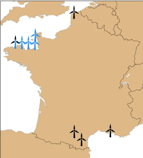
The selection of southern Greenland as the focus of this analysis is done via a MAR-based visual inspection of the entire Greenlandic land mass that reveals vast wind resource, relatively high temperatures and favourable topography for the subregion considered [30]. The locations sets used in the following analyses comprise geographical points which exist in both the ERA5 and MAR grids, respectively. In the following, the set of all locations in France is denoted by LF, while sites in South Greenland are grouped in LG. A third set, denoted by LF G, is defined as the union of the two aforementioned sets LF G = LF∪ LG . All aforementioned sets of locations are depicted in Figure 1.
4.2. Defining the Conversion Technology
The mapping of wind speeds to hourly average capacity factors is performed via a transfer function mimicking the normalised power output of a wind farm
comprising identical units which are geographically distributed in the direct vicinity of the site of interest. This approach is consistent with power system planning processes, where one is usually interested in developing wind farms rather than constructing a single turbine. As proposed in [32], such a trans-fer function is derived from the power curve of a representative wind turbine (the aerodyn SCD 8.0/168, in this particular case) by means of a Gaussian fit, where 100% availability of individual units is assumed (i.e., no down times due to maintenance, icing etc.). In addition, this specific wind energy converter is selected for illustration purposes only, regardless of its appropriateness for de-ployment at the locations considered. The result of this approach is depicted in Figure 2.
5. Results
This section presents a detailed discussion of results generated with the crit-icality indicator introduced in Section 3. Firstly, the values of the critcrit-icality indicator are examined for various instances of the (δ, α, β) triplet within the selected geographical areas. Then, the optimal deployment of generation sites in different geographical set-ups is discussed. Lastly, the current framework is leveraged to highlight potentially undesirable consequences of current power
Figure 1: Locations considered for the wind resource assessment in France and southern Greenland. The upper-left corner of the map displays the geographical points included in LG,
Figure 2: Single turbine and wind farm transfer functions associated with aerodyn SCD 8.0/168 units [31].
systems planning practices, which primarily favour electricity generation poten-tial and disregard the complementarity in electricity production regimes when selecting wind farm deployment sites.
5.1. Spatio-temporal Criticality Assessment
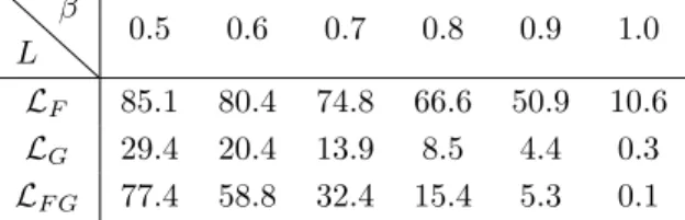
A comprehensive evaluation of wind resource complementarity in the avail-able locations sets over a time period spanning ten years (2008-2017) is first conducted using the criticality indicator. In the following example, as well as in all subsequent analyses, the local criticality threshold (α) is set to 35%, which is between the average capacity factors of the two regions computed from available data (i.e., 22% for all French sites and 48% for the locations in Greenland). The process of mapping wind signals to normalised power output values is done using the methodology introduced in Section 4.2. In other words, c(L) is computed for regions L ∈ {LF, LG, LF G}, local criticality threshold α = 0.35, window lengths δ ∈ {1, 24, 72, 168} and global criticality thresholds β ∈ {0.5, 0.6, . . . , 1.0}. The results of this analysis are shown in Figure 3.
First, as can be observed in all subplots of Figure 3, the value of the criticality indicator decreases as the global criticality threshold β increases, regardless of the time window length δ considered. This observation can be explained by observing that if the value of the global criticality threshold β is high, most locations must be critical for a time window to be counted as system-wide critical. Put differently, only a handful of non-critical locations are required for a time window not to be critical. In particular, for β = 1, all locations must be critical for the duration of a time window for the latter to be critical.
For all locations sets considered, taking β = 1.0 leads to values of the criticality indicator close to zero, which points to the existence of diversity in wind regimes even on a regional scale.
The change in criticality indicator values associated with the locations in France (LF) for different (δ, α, β) values is depicted in Figure 3a. For a time window length of 24 hours, as the global criticality threshold increases from 0.5 to 1.0, the proportion of critical windows drops from 85.1% (β = 0.5) to 66.6% (β = 0.8) and, finally, to 10.6% (β = 1.0). The same decreasing trend can be observed for all other δ values, with the score computed with the c index increasing as the window length is extended. Results corresponding to the
Figure 3: Criticality indicator c values for a local criticality threshold (i.e., α) of 35% for all locations in (a) France (LF), (b) Greenland (LG) and (c) the union of the two (LF G).
Table 1: Percent values of the criticality indicator c for various global criticality threshold values (β) and for all considered locations sets, considering a local criticality threshold (α) of 35% and a window length (δ) of 24 hours.
L β 0.5 0.6 0.7 0.8 0.9 1.0 LF 85.1 80.4 74.8 66.6 50.9 10.6 LG 29.4 20.4 13.9 8.5 4.4 0.3 LF G 77.4 58.8 32.4 15.4 5.3 0.1
available locations in Greenland are presented in Figure 3b. Superior resource quality in this region is evidenced by the range of criticality indicator values. For instance, in the case of a δ value of 24 hours, a drop in the proportion of critical time windows from 29.4% (for β = 0.5) to 8.5% (β = 0.8) and 0.3%, when β = 1.0, is observed. Contrary to the change in criticality indicator values for the locations in France, it can be seen that, for each global criticality threshold value, the criticality indicator values in Greenland decrease as the length of the time window increases. This phenomenon can be explained as follows. Recall that in this example, the mapping used to evaluate local resource quality computes an average value over the duration of each time window, which is then compared with the local criticality threshold. Since time windows overlap, for a given location, this procedure is essentially equivalent to the application of a moving average-based linear smoother to the original signal. More precisely, the longer the duration of the averaging window, the lower the frequency of the components left in the smoothed signal. Indeed, if a single time window spanning the full time horizon is considered, the smoothed signal reduces to a constant one whose value is the average capacity factor value at this location. Bearing in mind that the local criticality threshold value α was higher than the average capacity factor value in France and lower than the one computed in Greenland, it becomes clear that this shrinkage towards the mean as the time window duration increases leads to more instances of critical time windows in France and fewer instances of critical windows in Greenland.
Lastly, the outcome of coupling the two regions (LF and LG) is displayed in Figure 3c. Similarly to the case of Greenland, the criticality indicator de-creases as the time window length (δ) inde-creases. It should also be noted that, except for the β = 1.0 case, the criticality indices in Figure 3c are, for all (δ, β) configurations, smaller than the ones associated with the locations in France (LF) and greater than the ones corresponding to the sites in Greenland (LG). This can be explained by the fact that the influence of the inferior wind re-source in France is more pronounced for lower values of β. Nevertheless, the impact of the high-quality wind resource of Greenland is observed in the shape of the plotted curves which, compared with the ones computed for France (Fig-ure 3a), change curvat(Fig-ure, leading to a steeper drop of the c values as the β factor increases. Given a window length of 24 hours, the criticality indicator decreases from 77.4% (β = 0.5) to 15.4% (β = 0.8) and, to 0.1%, for a β value
of 1.0. These observations give a clear indication of the benefits of harvesting wind energy in Greenland in order to complement the existing wind regimes in France. For the sake of clarity, the output values of the criticality indicator for different locations sets, global criticality threshold values and considering a 24-hour time-window length are summarised in Table 1.
5.2. Optimal Deployment of Generation Sites
This subsection illustrates the optimisation model (5) introduced in Section 3.5. More specifically, the optimal deployment of n generation sites across k ar-eas is assessed for different regions (e.g., LF, LG, LF G), a given triplet (δ, α, β) and taking account of pre-defined constraints on the desired geographical repar-tition of wind farms throughout the k sub-regions. A time window length δ of 168 hours (one week), a local criticality threshold α of 35% and a global criti-cality threshold β of 1.0 are considered for illustrative purposes in the following example. A heuristic, which is described in detail in the supplementary mate-rial, is proposed to provide a suboptimal solution to the optimisation problem at hand, and results are shown in Figure 4.
The optimal deployment of five generation sites within the available locations in southern Greenland and continental France is shown in Figure 4a and Figure 4b, respectively. At first glance, it can be observed that the identified generation sites are evenly distributed over the regions of interest, again revealing (this time visually) the complementarity of wind regimes across dispersed locations, also on a regional scale. In addition, the actual wind farm locations in both cases can be explained by well-documented, prevailing local or regional wind regimes. In Greenland, the deployment of all but one wind farm is in line with the spatial occurrence of local katabatic flows [30]. In France, two wind farms are deployed in the resource-rich North, while the remaining ones are built in southern areas often swept by strong, local winds (the Mistral and Tramontane) [33]. The five locations in France display a 15% probability of critical window occurrence, while the superior quality of the wind resource in Greenland translates into an almost zero (0.4%) criticality indicator value.
The results of two variations on the same minimisation problem applied to the aggregated locations set (LF G) are discussed next. Figure 4c displays the optimal distribution of generation sites in France and Greenland without any deployment constraints. This variant corresponds to the case of a single, aggregated input region (i.e., k = 1). The proportion of one-week-long time windows with averaged capacity factor values across all five sites under 35% is only 0.005% over the full time horizon. Nevertheless, constraints on the geographical repartition of the generation sites can play a non-negligible role, as can be observed in Figure 4d. This plot shows the optimal deployment of the five sites considering the number of wind farms to be developed in Greenland is limited to two, in which case the criticality indicator score increases to 0.06%. 5.3. Comparison with Average Capacity Factors as Deployment Criterion
It is particularly insightful to compare deployment patterns resulting from the use of different siting criteria. In particular, the usual criterion used for wind
Figure 4: Visualisation of the optimal deployment of five wind farms in (a) Greenland, (b) France, (c) the aggregation of the two without and (d) with constraints on the geographical15
farm deployment is the generation potential (or the average capacity factor) of the site. A comparison between this indicator and the complementarity criterion proposed in this paper is presented in Figure 5 for the case of France. In this plot, the black markers are associated with the solution of the minimisation problem (5). The blue ones correspond to the five best locations in LF (see Figure 1), strictly from a generation potential perspective (i.e., locations are ranked based on integrated capacity factor values over the entire time horizon considered). The point displayed in both colours represents a generation site common to both solutions.
The minimisation problem returns a deployment pattern whose criticality indicator value stands at roughly 0.15, which corresponds to a 15% probability of observing simultaneous low-production events. The criticality indicator value associated with the five most productive sites is much higher (23.6%). In other words, for a capacity factor threshold of 35% and compared with the locations set identified through the minimisation problem, the likelihood of recording a 168-hour long critical window across the five most productive sites is 60% higher. This increase stems from the geographical proximity of the locations, which makes them subject to very similar wind regimes. However, the improvement in criticality indicator value for the locations with highest complementarity comes at the expense of total annual output. While the five most productive wind farms boast an aggregated capacity factor value of 46% over the entire time horizon considered, the locations with highest complementarity only have an aggregated capacity factor value of 34%.
Overall, these results suggest that a trade-off exists between high production levels and a reduced occurrence of simultaneous low-production events, and such considerations should be accounted for in planning decisions and incentive schemes.
5.4. Results Discussion
A key factor impacting the accuracy of results presented in Section 5 is the accuracy of the raw data used throughout the analysis. In this respect, it has been previously shown that significant spatial bias is sometimes introduced by reanalysis models, which limits their ability to recreate VRES patterns in certain topographies [32]. This undesirable feature is also observed in the current study that uses the ERA5 reanalysis database. Comparing modelled average capacity factors (as computed from ERA5 resource data) with field data gathered in the regions where the generation sites in Figure 5 are located, non-negligible differences can be observed. On the one hand, for the locations in southern France, the computed average capacity factor is close to 25%, a value which is close to the official statistics (27.4% in 2016) [34]. On the other hand, a clear positive bias of the reanalysis model can be observed for the six locations in northern France. For these locations, a modelled average capacity factor of 45% is significantly higher than the reported 19 to 22% values associated with the corresponding French regions in 2016 [34], but it seems unlikely that the aforementioned bias alone leads to such a substantial difference. At any rate, the sole purpose of the wind database used in this work is to illustrate the
Figure 5: Comparison of criticality indicator-based (black) and electricity yield-based (blue) deployment of wind farms within a given subset of locations, based on the criticality indicator values. Example depicting the results for the subset of potential generation sites in France, LF.
Table 2: Influence of the local criticality threshold (α) on the trade-off between criticality in-dicator gain and average capacity factor loss in the context of deployment strategy comparison between (i) criticality indicator minimisation and (ii) average capacity factor as deployment criterion. Numerical results displayed for one-week-long time windows (δ = 168) and a global criticality threshold (β) of 1.0.
α - 0.15 0.35 0.40 0.45 0.65
∆c % -99.6 -36.4 -27.6 -20.4 -1.9
∆u % -28.2 -26.0 -26.0 -26.0 -16.6
mathematical framework proposed in Section 3 and the continuous improvement of reanalysis models over the years suggests that these tools could be used more reliably in such applications in the near future. Nevertheless, final decisions on wind farm site selection should be confirmed by extensive in-situ measurements. One interesting implication of the proposed methodology stems from the re-sults presented in Section 5.3, which suggest the existence of a trade-off between maximising energy volumes and minimising the occurrence of system-wide low production events when deploying VRES generation. Since such events directly impact the planning and operation of power systems, developing regulatory frameworks incentivising producers to provide system-level services (e.g. taking advantage of VRES regime diversity to contribute to a base load provision of electricity) may prove beneficial in power systems relying heavily on renewable power generation.
Table 2 provides additional insight into how the local criticality threshold value influences the properties of the deployment patterns obtained via (5), and how these properties compare with those of the deployment pattern maximis-ing annual electricity output. More precisely, each entry in the second row shows the relative difference in criticality indicator values between the deploy-ment pattern maximising compledeploy-mentarity and the one maximising electricity output, respectively. Thus, each entry expresses the change in the number of critical time windows between deployment patterns, and a negative sign in-dicates that the pattern maximising complementarity has fewer critical time windows. Then, the third row gives the relative difference in average capacity factor values. A negative sign indicates that the power generation potential of the deployment pattern maximising complementarity is lower than that of the pattern maximising electricity output. Now, inspecting the second row reveals that the change in criticality indicator values becomes smaller as the value of the local criticality threshold increases. In other words, a deployment pattern produced by (5) for a high value of the local criticality threshold has a num-ber of critical time windows roughly equal to that observed for the deployment pattern maximising electricity output. A similar trend is observed in the third row. It therefore appears that the deployment patterns produced by (5) con-verge towards the deployment pattern maximising electricity output as the local criticality threshold value increases. It is also worth noting that, in contrast to the differences in criticality indicator values, the differences in average capacity
factor values remain constant over a range of α values. This observation sug-gests that deployment patterns displaying the same level of annual electricity output can exhibit different levels of complementarity. Hence, the method de-veloped in this paper also allows for the identification of deployment patterns maximising complementarity within a subset of locations with a pre-specified level of electricity output, which can be simply achieved by tuning the local criticality threshold parameter.
6. Conclusion and Future Work
A framework to systematically assess the complementarity of dispersed vari-able renewvari-able energy resources over arbitrary time scales has been presented. The framework relies on the concept of critical time windows, which provide an accurate, time-domain description of low-probability VRES power genera-tion events impacting power system operagenera-tion and planning. A scalar indicator quantifying the complementarity dispersed VRES generation sites may exhibit is derived, providing a practical tool to evaluate the respective merits of differ-ent VRES deploymdiffer-ent patterns. This indicator is also leveraged to formulate optimisation problems seeking to identify deployment patterns with the smallest occurrence of low production events within a region of interest.
The usefulness of the proposed framework is illustrated in a case study inves-tigating the complementarity between wind regimes within and across continen-tal France and southern Greenland. The analysis reveals that a reduction in the occurrence of system-wide low VRES generation events can be achieved when the two areas are spatially aggregated, pointing to potential benefits of an in-tercontinental electrical interconnection linking the two regions. Moreover, the solutions to optimisation problems derived from the criticality indicator show that the occurrence of low power production events can also be reduced on a re-gional scale by exploiting the diversity in local wind regimes. In essence, results confirm the intuition that deploying generation sites across continents makes it possible to simultaneously take advantage of high-quality resources and exploit the greater diversity in wind regimes in order to reduce the occurrence of simul-taneous low power generation events. The relevance of the proposed methodol-ogy in a power systems planning context is further supported by a comparison of two wind farm deployment strategies favouring complementarity and seeking to maximise annual electricity output, respectively. These two approaches, which were tested in continental France, yield starkly different deployment patterns, with implications for planning strategies in future power systems dominated by vast shares of renewable-based generation, where maintaining adequate lev-els of security of electricity supply may require a comprehensive assessment of renewable resource complementarity.
Several research avenues can be pursued in future work. For instance, a straightforward extension of the present analysis would consist in applying the framework to investigate the complementarity between different renewable re-source types across much greater geographical areas, possibly spanning several
continents simultaneously. From a computational standpoint, recasting the pro-posed optimisation problems in a more structured form would be beneficial, as it would allow for the use of efficient off-the-shelf solvers, e.g. branch-and-bound, which would provide certificates of optimality. If such efforts prove fruitless, a comprehensive analysis and extension of the proposed heuristic to cases in which β 6= 1 would be needed. Finally, further exploring the trade-off between maximising complementarity and annual electricity output would be particu-larly useful for planning purposes. More precisely, quantifying the value of complementarity in economic terms would make it possible to identify whether transmission, dispatchable generation or storage capacity expansion strategies should be pursued to ensure adequacy in a power system with very high shares of variable renewable resources. In the same vein, updating the optimisation problems to include other constraints and costs, for instance reflecting a desired level of installed renewable generation capacity or the difficulty to connect to existing infrastructure, would allow for a more complete assessment of renewable generation deployment options.
Nomenclature
α local criticality threshold β global criticality threshold δ time window duration
c mapping associating its criticality indicator to any set of locations CL set of critical time windows for locations set L
cL criticality indicator of locations set L
fl transfer function of candidate technology at location l JL
w subset of locations in L that are critical over time window w k subregion index
K number of subregions L set of all locations
L subset of locations, i.e., L ⊆ L l individual location, i.e., l ∈ L n number of desired deployments
nk number of desired deployments in subregion k NL
w number of locations in L that are critical over time window w q resource quality mapping
qlw local resource quality score at location l, over window w T set of time periods in discretised time horizon
t time period index
sl resource signal time series at location l ul capacity factor time series at location l ul
w truncation of capacity factor time series ulover time window w W set of time windows
wδ
t time window of duration δ starting at time period t
References
[1] S. Chatzivasileiadis, D. Ernst, G. Andersson, The global grid, Renewable Energy 57 (2013) 372–383.
[2] J. Jurasz, F. Canales, A. Kies, M. Guezgouz, A. Beluco, A review on the complementarity of renewable energy sources: Concept, metrics, applica-tion and future research direcapplica-tions, Solar Energy 195 (2020) 703 – 724. doi:https://doi.org/10.1016/j.solener.2019.11.087.
[3] ECMWF, Copernicus knowledge base - ERA5 data documentation, https://confluence.ecmwf.int//display/CKB/ (2018).
[4] K. Engeland, M. Borga, J.-D. Creutin, B. Fran¸cois, M.-H. Ramos, J.-P. Vi-dal, Space-time variability of climate variables and intermittent renewable electricity production – a review, Renewable and Sustainable Energy Re-views 79 (2017) 600 – 617. doi:https://doi.org/10.1016/j.rser.2017.05.046. [5] G. Giebel, On the benefits of distributed generation of wind energy in
Europe, PhD thesis, University of Oldenburg, Germany (Jul 2001). [6] J. Olauson, M. Bergkvist, Correlation between wind power
gener-ation in the european countries, Energy 114 (2016) 663 – 670. doi:https://doi.org/10.1016/j.energy.2016.08.036.
[7] K. Klima, J. Apt, Geographic smoothing of solar PV: results from Gujarat, Environmental Research Letters 10 (10) (2015) 104001.
[8] S. Sterl, S. Liersch, H. Koch, N. P. M. van Lipzig, W. Thiery, A new approach for assessing synergies of solar and wind power: implications for west africa, Environmental Research Letters 13 (9). doi:10.1088/1748-9326/aad8f6.
[9] J. H. Slusarewicz, D. S. Cohan, Assessing solar and wind complemen-tarity in texas, Renewables: Wind, Water, and Solar 5 (1) (2018) 7. doi:10.1186/s40807-018-0054-3.
[10] J. Jurasz, A. Beluco, F. A. Canales, The impact of complementarity on power supply reliability of small scale hybrid energy systems, Energy 161 (2018) 737 – 743. doi:https://doi.org/10.1016/j.energy.2018.07.182. [11] J. Widen, Correlations between large-scale solar and wind power in a future
scenario for Sweden, IEEE Transactions on Sustainable Energy 2 (2) (2011) 177–184. doi:10.1109/TSTE.2010.2101620.
[12] P. E. Bett, H. E. Thornton, The climatological relationships between wind and solar energy supply in Britain, Renewable Energy 87 (2016) 96 – 110. doi:https://doi.org/10.1016/j.renene.2015.10.006.
[13] M. M. Miglietta, T. Huld, F. Monforti-Ferrario, Local complementarity of wind and solar energy resources over europe: An assessment study from a meteorological perspective, Journal of Applied Meteorology and Climatol-ogy 56 (1) (2017) 217–234. doi:10.1175/JAMC-D-16-0031.1.
[14] P. S. dos Anjos, A. S. A. da Silva, B. Stosic, T. Stosic, Long-term correlations and cross-correlations in wind speed and solar radi-ation temporal series from Fernando de Noronha Island, Brazil, Phys-ica A: StatistPhys-ical Mechanics and its ApplPhys-ications 424 (2015) 90 – 96. doi:https://doi.org/10.1016/j.physa.2015.01.003.
[15] G. Ren, J. Wan, J. Liu, D. Yu, Spatial and temporal assessments of com-plementarity for renewable energy resources in china, Energy 177 (2019) 262 – 275. doi:https://doi.org/10.1016/j.energy.2019.04.023.
[16] H. Louie, Correlation and statistical characteristics of aggregate wind power in large transcontinental systems, Wind Energy 17 (6) (2013) 793–810. doi:10.1002/we.1597.
[17] C. M. S. Martin, J. K. Lundquist, M. A. Handschy, Variability of intercon-nected wind plants: correlation length and its dependence on variability time scale, Environmental Research Letters 10 (4).
[18] C. E. Hoicka, I. H. Rowlands, Solar and wind resource complementarity: Advancing options for renewable electricity integration in Ontario, Canada, Renewable Energy 36 (1) (2011) 97 – 107.
[19] F. Monforti, T. Huld, K. B´odis, L. Vitali, M. D’Isidoro, R. Lacal-Ar´antegui, Assessing complementarity of wind and solar resources for energy produc-tion in Italy. a Monte Carlo approach, Renewable Energy 63 (2014) 576 – 586. doi:https://doi.org/10.1016/j.renene.2013.10.028.
[20] H. Zhang, Y. Cao, Y. Zhang, V. Terzija, Quantitative synergy assessment of regional wind-solar energy resources based on MERRA reanalysis data, Applied Energy 216 (2018) 172 – 182. doi:10.1016/j.apenergy.2018.02.094. [21] W. Li, S. Stadler, R. Ramakumar, Modeling and assessment of wind and insolation resources with a focus on their complementary nature: A case study of Oklahoma, Annals of the Association of American Geographers 101 (4) (2011) 717–729. doi:10.1080/00045608.2011.567926.
[22] J. Apt, The spectrum of power from wind turbines,
Journal of Power Sources 169 (2) (2007) 369 – 374.
doi:https://doi.org/10.1016/j.jpowsour.2007.02.077.
[23] W. Katzenstein, E. Fertig, J. Apt, The variability of interconnected wind plants, Energy Policy 38 (8) (2010) 4400–4410.
[24] A. A. Prasad, R. A. Taylor, M. Kay, Assessment of solar and wind resource synergy in australia, Applied Energy 190 (2017) 354 – 367. doi:https://doi.org/10.1016/j.apenergy.2016.12.135.
[25] G. Ren, J. Wan, J. Liu, D. Yu, Characterization of wind resource in china from a new perspective, Energy 167 (2019) 994 – 1010. doi:https://doi.org/10.1016/j.energy.2018.11.032.
[26] A. Beluco, P. K. de Souza, A. Krenzinger, A dimensionless in-dex evaluating the time complementarity between solar and hy-draulic energies, Renewable Energy 33 (10) (2008) 2157 – 2165. doi:https://doi.org/10.1016/j.renene.2008.01.019.
[27] S. Rose, J. Apt, What can reanalysis data tell us about wind power?, Renewable Energy 83 (2015) 963–969.
[28] J. Olauson, ERA5: The new champion of wind power modelling?, Renew-able Energy 126 (2018) 322–331.
[29] X. Fettweis, J. E. Box, C. Agosta, C. Amory, C. Kittel, C. Lang, D. van As, H. Machguth, H. Gall´ee, Reconstructions of the 1900–2015 Greenland ice sheet surface mass balance using the regional climate MAR model, The Cryosphere 11 (2) (2017) 1015.
[30] D. Radu, M. Berger, R. Fonteneau, S. Hardy, X. Fettweis, M. L. Du, P. Pan-ciatici, L. Balea, D. Ernst, Complementarity assessment of south greenland katabatic flows and west europe wind regimes, Energy 175 (2019) 393 – 401. doi:https://doi.org/10.1016/j.energy.2019.03.048.
[31] Aerodyn Engineering GMBH, SCD 8.0 MW – Technical Data, Tech. rep., Aerodyn Engineering GMBH (2018).
[32] I. Staffell, S. Pfenninger, Using bias-corrected reanalysis to simulate current and future wind power output, Energy 114 (2016) 1224–1239.
[33] A. Obermann, S. Bastin, S. Belamari, D. Conte, M. A. Gaertner, L. Li, B. Ahrens, Mistral and Tramontane wind speed and wind direction patterns in regional climate simulations, Climate Dynamics 51 (2016) 1059–1076. [34] RTE, Bilan ´electrique et perspectives - Bretagne/Hauts de

![Figure 2: Single turbine and wind farm transfer functions associated with aerodyn SCD 8.0/168 units [31].](https://thumb-eu.123doks.com/thumbv2/123doknet/6530558.175561/11.918.208.711.191.493/figure-single-turbine-transfer-functions-associated-aerodyn-units.webp)