HAL Id: in2p3-00022236
http://hal.in2p3.fr/in2p3-00022236
Submitted on 15 Jan 2007
HAL is a multi-disciplinary open access
archive for the deposit and dissemination of
sci-entific research documents, whether they are
pub-lished or not. The documents may come from
teaching and research institutions in France or
abroad, or from public or private research centers.
L’archive ouverte pluridisciplinaire HAL, est
destinée au dépôt et à la diffusion de documents
scientifiques de niveau recherche, publiés ou non,
émanant des établissements d’enseignement et de
recherche français ou étrangers, des laboratoires
publics ou privés.
First identification and modelling of SPI background
lines
G. Weidenspointner, J. Kiener, M. Gros, P. Jean, Bj. Teegarden, C.
Wunderer, R.C. Reedy, D. Attie, R. Diehl, C. Ferguson, et al.
To cite this version:
G. Weidenspointner, J. Kiener, M. Gros, P. Jean, Bj. Teegarden, et al.. First identification and
modelling of SPI background lines. Astronomy and Astrophysics - A&A, EDP Sciences, 2003, 411,
pp.L113-L116. �10.1051/0004-6361:20031209�. �in2p3-00022236�
A&A 411, L113–L116 (2003) DOI: 10.1051/0004-6361:20031209 c ESO 2003
Astronomy
&
Astrophysics
First identification and modelling of SPI background lines
?,??
G. Weidenspointner
1,2,3, ???, J. Kiener
4, M. Gros
5, P. Jean
3, B. J. Teegarden
1, C. Wunderer
6, R. C. Reedy
3,7,
D. Atti´e
5, R. Diehl
6, C. Ferguson
8, M. J. Harris
1,2, J. Kn¨odlseder
3, P. Leleux
9, V. Lonjou
3, J.-P. Roques
3,
V. Sch¨onfelder
6, C. Shrader
1,2, S. Sturner
1,2, V. Tatische
ff
4, and G. Vedrenne
31 NASA Goddard Space Flight Center, LHEA, Code 661, Greenbelt, MD 20771, USA
2 Universities Space Research Association, 7501 Forbes Blvd. #206, Seabrook, MD 20706, USA 3 Centre d’ ´Etude Spatiale des Rayonnements, 9 avenue Colonel Roche, 31028 Toulouse Cedex 4, France 4 CSNSM, IN2P3-CNRS and Universit´e Paris-Sud, 91405 Orsay, France
5 DSM/DAPNIA/SAp, Centre d’ ´Etudes Nucl´eaires de Saclay, 91191 Gif-sur-Yvette Cedex, France 6 Max-Planck-Institut f¨ur extraterrestrische Physik, Giessenbachstrasse, 85740 Garching, Germany 7 University of New Mexico, Albuquerque, NM 87131, USA
8 Department of Physics and Astronomy, University of Southampton, Southampton SO17 1BJ, UK 9 Institut de Physique Nucl´eaire, Universit´e catholique de Louvain, 1348 Louvain-la-Neuve, Belgium
Received 16 July 2003/ Accepted 4 August 2003
Abstract.On Oct. 17, 2002, the ESA INTEGRAL observatory was launched into a highly elliptical orbit. SPI, a high resolution Ge spectrometer covering an energy range of 20–8000 keV, is one of its two main instruments. We use data recorded early in the mission (i.e. in March 2003) to characterize the instrumental background, in particular the many gamma-ray lines produced by cosmic-ray interactions in the instrument and spacecraft materials. More than 300 lines and spectral features are observed, for about 220 of which we provide identifications. An electronic version of this list, which will be updated continuously, is available for download at CESR. We also report first results from our efforts to model these lines by ab initio Monte Carlo simulation.
Key words.line: identification – instrumentation: miscellaneous – methods: data analysis – methods: numerical
1. Introduction
The Spectrometer for INTEGRAL (SPI) is one of the two main instruments on board ESA’s INTEGRAL observatory launched from Baikonour, Kazakhstan, on Oct. 17, 2002. The INTEGRAL mission was placed into a highly elliptical orbit with a perigee of 9000 km. Consequently, INTEGRAL does not benefit from geomagnetic shielding and is fully exposed to all cosmic rays. Interactions of these cosmic rays within the instrument and spacecraft materials are the dominant source of instrumental background for SPI. In particular, delayed de-cays of radio-isotopes and prompt de-excitations of excited nu-clei produced in nuclear interactions give rise to a plethora of
Send offprint requests to: G. Weidenspointner,
e-mail: [email protected]
? Based on observations with INTEGRAL, an ESA project with instruments and science data centre funded by ESA member states (especially the PI countries: Denmark, France, Germany, Italy, Switzerland, Spain), Czech Republic and Poland, and with the par-ticipation of Russia and the USA.
?? Table 1 is only available in electronic form at
http://www.edpsciences.org
??? Present address: Centre d’ ´Etude Spatiale des Rayonnements, 9 avenue Colonel Roche, BP 4346, 31028 Toulouse Cedex 4, France.
instrumental lines which are the focus of this work. The general characteristics of the SPI instrumental background and its tem-poral and orbital variation are described by Jean et al. (2003).
A detailed understanding of the instrumental lines is valu-able for both the operation of the instrument as well as for scientific analyses. Accurate line identifications are a prere-quisite for the absolute energy calibration of the detectors and the monitoring of their radiation damage. Many scientific analyses, in particular studies of diffuse gamma-ray emission from the Galaxy, necessitate modelling both the amplitude and shape of the instrumental background in specific energy re-gions. Typically, this involves modelling of instrumental lines.
2. Instrument description and data analysis
The SPI spectrometer consists of an array of 19 actively cooled high resolution Ge detectors with a total volume of 3396 cm3.
The detectors cover an energy range of 20–8000 keV at an en-ergy resolution of about 2.5 keV full width at half maximum (FHWM) at 1.1 MeV. SPI employs an active anti-coincidence shield made of bismuth germanate (BGO), which also acts as a collimator. Detailed descriptions of the instrument, its ground
Letter
to
the
L114 G. Weidenspointner et al.: First identification and modelling of SPI background lines calibration, and in-flight performance are given by Vedrenne
et al. (2003); Atti´e et al. (2003); Roques et al. (2003).
The data used in this investigation were recorded in March 2003 (i.e. during revolutions 49, 50, 51, and 53). During this time the variation of the temperature of the Ge detectors and their electronics, and consequently the gain drift, was su ff-ciently small to allow us to use a single energy calibration for the combined data. Also, these revolutions followed shortly af-ter the first detector annealing, hence the energy resolution of the detectors was close to optimal (see Roques et al. 2003). An absolute energy calibration was obtained by first summing all data for each detector and by assuming a quadratic relation be-tween channel number and energy for both the low (up to about 2 MeV) and high gain range (above about 2 MeV). We found this calibration to be accurate to within about 0.2 keV for most energies, and slightly less accurate at the lowest (below about 200 keV) and the highest (above a few MeV) energies. All fits were performed using the GASPAN1gamma spectrum analysis
program. We found that a Gaussian, with its width constrained at the instrumental resolution, provided an adequate description of the line shape at all energies.
The event types used in this study consist of single detector events (events that deposited energy in only one detector), dou-ble and triple events (events that involve coincident interactions in two or three detectors), and so-called broken double events (the energy deposits in individual detectors for double events). A detailed description of the various SPI event types is given in Roques et al. (2003), Vedrenne et al. (2003).
3. Line identifications and characteristics
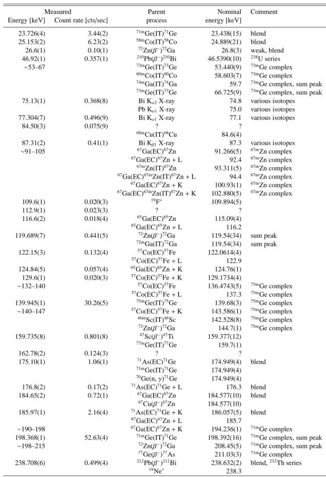
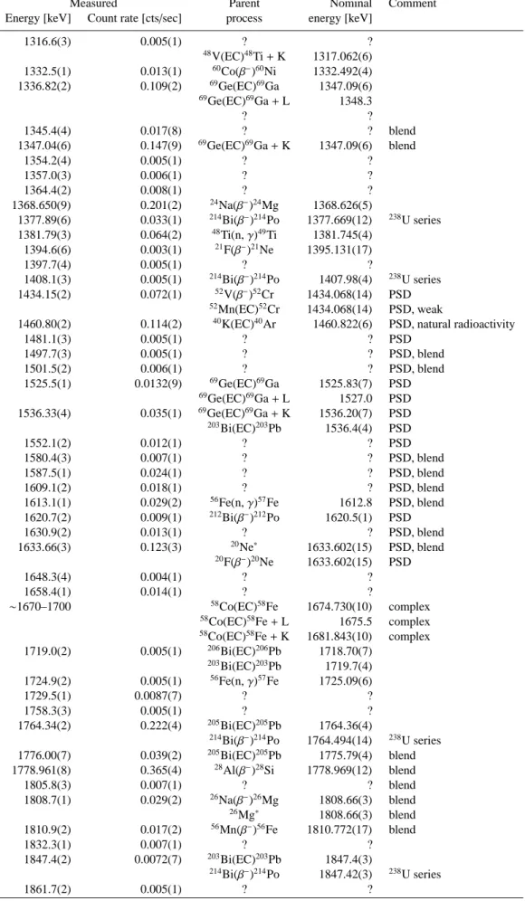
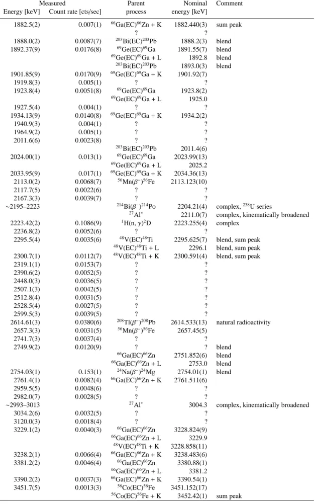
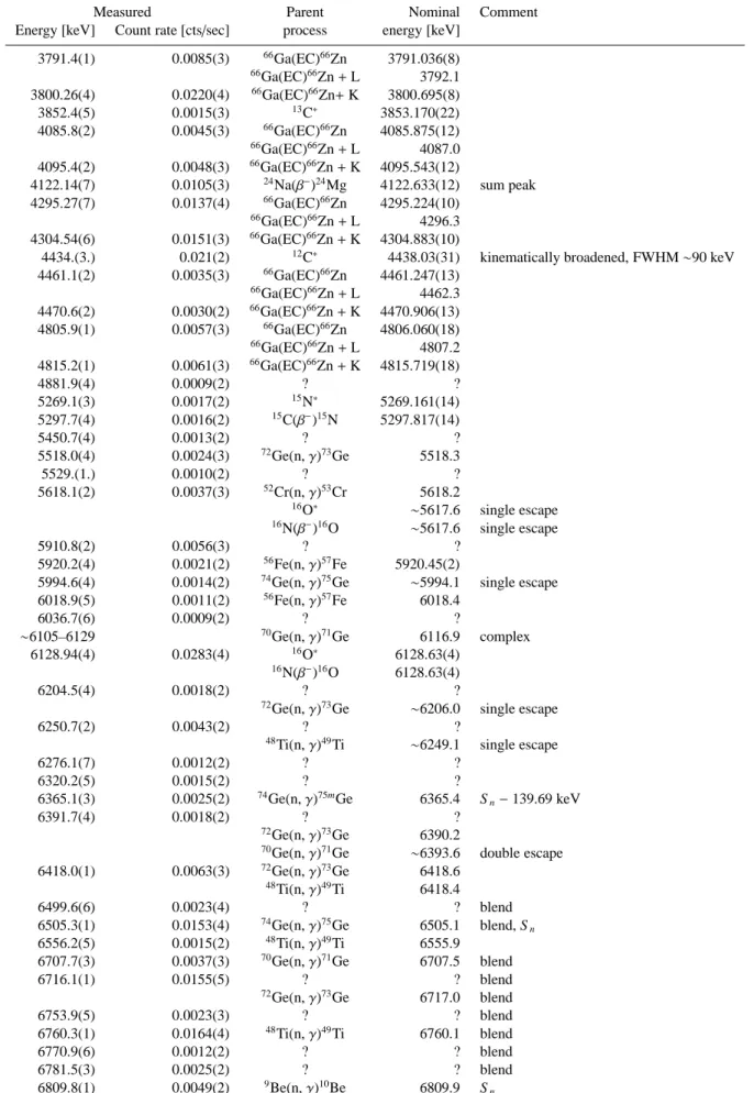
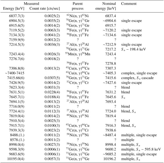
The analysis and identification of the more than 300 instrumen-tal lines and spectral features is an on-going process; Table 1 summarizes our current knowledge. An electronic version of the table, which will continuously be updated as our under-standing advances, is available at CESR2. Up to 8 MeV the table entries refer to single detector events3. Combining coinci-dent energy deposits in multiple detectors allows us to observe lines above 8 MeV. The quoted line count rates represent the sum over the full detector array.
Table 1 is organized in five columns. The first two columns provide energy and count rate of the observed line or spec-tral feature; the quoted errors are statistical only. Columns three and four provide, if possible, the identified parent pro-cess and the nominal energy of the line or feature based on evaluated nuclear data available at the Brookhaven National Laboratory4 and, in addition for lines from (n, γ) reactions,
1 The software, developed by F. Riess, and
documenta-tion are available under http://ftp.leo.org/download/ pub/science/physics/software/gaspan/
2 http://sigma-2.cesr.fr/spi/download/
spi intrumental lines/
3 In 1.4–1.6 MeV only single detector events that also triggered the
PSD electronics have been used to avoid electronic noise; the count rates were corrected for the efficiency of the PSD electronics which at these energies is about 85% (see Roques et al. 2003).
4 http://www.nndc.bnl.gov/
on Frankle et al. (2001); Reedy & Frankle (2002). The com-ments in column five are intended to provide supplementary information.
We have not applied a strict and uniform criterion on the statistical significance of lines for inclusion in the table. For unidentified features, indicated by question marks in columns three and four, the significance is about 5σ. However, if we have reason to believe in the reality of a weak line or feature based on identified stronger lines and known branching ratios, then these are listed as well. If we have reason to believe that multiple processes contribute to a single line or feature, then these are listed in the order of their (suspected) contribution. In some cases we suspect a yet unidentified partial contribu-tion to a line, which we again indicate with quescontribu-tion marks. The measured line energy and rate are listed only for the first contributor.
Despite the excellent energy resolution of SPI there are many regions in the spectrum where a few or even several closely spaced lines blend to form a broad line or feature, or where lines and instrinsically broad features merge. These re-gions are indicated in the table. In particular for complex fea-tures it can be very difficult to determine reliable values for contributing lines. At this early stage of the analysis we then limit ourselves to merely listing identified contributors, without quoting values in the first two columns. Especially for com-plex regions the list of contributors can not assumed to be exhaustive.
We followed a variety of approaches to arrive at the line identifications in Table 1. All identifications required close agreement between the measured energy and the nominal en-ergy of the parent process. Processes involving proton and neutron interactions had to be plausible considering the ma-terial composition of instrument and spacecraft and the parti-cle fluxes and cross-sections. The Monte Carlo simulations de-scribed in Sect. 4 were particularly helpful in this respect. For decays that result in the emission of multiple photons consis-tency was required between observed and expected line ratios. Again, Monte Carlo simulations were very helpful, especially for decays within or close to the veto shield or the Ge detectors. We also consulted compilations of instrumental lines seen in other high resolution Ge spectrometers flown in space, such as on HEAO-3 (Wheaton et al. 1989), the TGRS on board WIND (Weidenspointner et al. 2003), and on Mars Odyssey (Evans et al. 2002), as well as on balloons such as GRIS (Bartlett 1994) and HIREGS (Feffer 1996).
The strength of some of the listed lines varies with time; the quoted values represent an average for March 2003. For lines from prompt de-excitations or the decay of short-lived isotopes the main cause for time variability is the variation of the am-bient cosmic radiation. For lines from the decay of long-lived isotopes the variability of the line strength is mainly due to the interplay of activation and radioactive decay. This should be taken into consideration when trying to predict line strengths in the future. Also, there can be significant differences in the line strength between individual detectors (see Jean et al. 2003, for more details on background variations).
A particularly abrupt change in the ambient radiation en-vironment occurs during times when INTEGRAL is exposed
Letter
to
the
G. Weidenspointner et al.: First identification and modelling of SPI background lines L115
Fig. 1. A comparison of simulated
SPI single detector events with ac-tual flight data. Details are given in the text. The broad spikes in the data in 1.4–1.6 MeV are electronic noise.
to solar energetic particles. Regarding the SPI background lines, the most important effect of solar energetic particles is to greatly increase the strengths of lines due to inelastic proton scattering (e.g. on Al and C). In some cases lines which are too weak in the “quiescent” background become detectable during a solar event. The time variation of these lines follows closely the intensity of the solar proton flux. A more detailed discus-sion of the effect of solar energetic particles on the background of SPI is beyond the scope of this paper and will be presented elsewhere (see also Jean et al. 2003).
An important part of the background lines arises from de-cays of isomers or from EC dede-cays of radio-isotopes produced by spallation and neutron capture reactions inside the Ge crys-tals. In general, an isomer decays by internal transition to its ground state and produces a single background line. However, if the half-life of an isomeric level is similar to the peaking timeτ of the electronic, which for SPI is about 8 µs, and if the isomeric level is part of a cascade, then this cascade gives rise to a double-horn structure in the spectrum. For SPI this is the case for67mZn and73mGe inside the Ge detectors. The in-terpeak region is due to an electronic effect which results in a partial summation of two energy deposits that are aboutτ apart in time. The detailed dependence of the double-horn shape on the electronic time constants and the de-excitation cascade is complicated. Gamma-ray transitions in the daughter nucleus following EC decay inside the Ge crystals appear at two dis-tinct energies, depending on the shell from which the electron was captured and on whether the gamma ray and electron bind-ing energies are summed. The first EC feature is a blend of two components: gamma rays at the nominal transition energy5, and
gamma rays summed with the electron binding energy for cap-tures from above the K shell (labelledAAZZ(EC) + L in the
table). The proportion of the different contributions is difficult to estimate. The second EC feature (labelledAAZZ(EC) + K) is from K-shell capture in the crystal detecting the gamma ray,
5 ECs outside the detectors contribute as well.
the energy of the gamma ray line being shifted by the K-shell electron binding energy.
Above 5 MeV, with the exception of the16N(β−)16O decay
and16O∗line, all lines are due to capture reactions of low en-ergy neutrons in the Ge crystals or surrounding material. The positions and widths of these lines suggest that they were pro-duced by capture of thermal neutrons.
4. Background modelling
We employed the MGGPOD suite in an attempt to model the SPI instrumental background, in particular the many gamma ray lines, by Monte Carlo simulation. In a nutshell, the MGGPOD suite was developed to simulate ab initio the physi-cal processes relevant for the production of instrumental back-grounds. These include the build-up and delayed decay of ra-dioactive isotopes as well as the prompt de-excitation of excited nuclei, both of which give rise to a plethora of instrumental gamma-ray background lines in addition to continuum back-grounds. A detailed description of the MGGPOD suite can be found in Weidenspointner et al. (2003).
A Monte Carlo simulation of instrumental backgrounds re-quires a mathematical representation of the instrumental set-up (the so-called mass model) and a model of the radiation en-vironment. In our simulation we combined the very detailed mass model of the SPI instrument developed at NASA/GSFC (see Sturner et al. 2003) with “The INTEGRAL Mass Model” (TIMM) developed at the University of Southampton (Ferguson et al. 2003) which describes the spacecraft and the other instruments on board. The radiation environment con-sisted of two components: the cosmic X and gamma radiation was modelled according to Gruber et al. (1999); the Galactic cosmic-ray proton spectrum, corrected for solar modulation, was based on the models of Moskalenko et al. (2002).
A comparison of a MGGPOD simulation of SPI single detector events with actual flight data (an empty field ob-servation during Rev. 13) is depicted in Fig. 1. It has to be
Letter
to
the
L116 G. Weidenspointner et al.: First identification and modelling of SPI background lines emphasized that in this simulation the PROMPT package,
which in the framework of MGGPOD is used for modelling prompt gamma-ray line emission after spallation, neutron cap-ture, and inelastic neutron scattering (see Weidenspointner et al. 2003), has not been included. The simulation comprises three background components: background events due to extra-galactic X and gamma rays (blue), prompt background events resulting from nuclear interactions of cosmic-ray protons in spacecraft and instrument (green), and background events that arise from the delayed radioactive decay of radio-isotopes pro-duced in nuclear interactions of cosmic-ray protons and their hadronic secondaries (purple). The sum of these three compo-nents is depicted in red; the actual flight data are represented by the black spectrum. A similar comparison between a simulated background spectrum, obtained with the GGOD Monte Carlo suite, and SPI data is shown in Ferguson et al. (2003).
As can be seen in Fig. 1, the MGGPOD simulation repro-duces well the overall shape and magnitude of the continuum background, and also reproduces well many lines from radioac-tive decays. Special attention has been given to the numerous lines that result from decays involving isomeric levels, partic-ularly in the Ge detectors. The simulation accounts for 71% of the observed total 20–8000 keV count rate. Below 4 MeV the simulation never falls short of the data by more than a fac-tor of 2. At higher energies, where gamma rays from (thermal) neutron capture are important, but not yet included in the sim-ulation, the difference can be larger. The lines from radioactive decays which are produced in the simulation provided very use-ful information for our line identification efforts (see Sect. 3). Modelling the SPI instrumental background by Monte Carlo simulation is an ongoing effort. A more detailed description and comparison will be presented in a forthcoming publication.
5. Discussion
SPI employs a large Ge detector array with a massive BGO anti-coincidence shield on board a heavy spacecraft. The confluence of these factors results in an instrumental back-ground that is very rich in lines and spectral features for which we provide first identifications. The main contributor to this background, both line and continuum, are radioactive decays, particularly within the Ge crystals, nearby materials, and the
BGO shield. Spallation and neutron activation are the dominant source of activation, as has been found for previous Ge spec-trometers (see e.g. Wheaton et al. 1989; Evans et al. 2002). These decays are well reproduced by ab initio Monte Carlo simulation using the MGGPOD suite. Thermal neutron capture is responsible for numerous and strong lines at several MeV; their unexpected presence poses a difficult challenge for our physical understanding of instrumental backgrounds and for Monte Carlo codes such as MGGPOD. Both the analysis and identification as well as the modelling of the line background are work in progress. We expect to present more detailed results in the future.
Acknowledgements. The SPI project has been completed under the
responsibility and leadership of CNES. We are grateful to ASI, CEA, CNES, DLR, ESA, INTA, NASA and UCL for their support.
References
Atti´e, D., Cordier, B., Gros, M., et al. 2003, 411, L71
Bartlett, L. M. 1994, Ph.D. Thesis, University of Maryland, USA Diehl, R., Baby, N., Beckmann, V., et al. 2003, 411, L117
Evans, L. G., Boynton, W. V., Reedy, R. C., et al. 2002, Proc. of SPIE 4784, X-Ray and Gamma-Ray Detectors and Applications IV, 31 Feffer, P. T. 1996, Ph.D. Thesis, University of California Berkeley,
CA 94720, USA
Ferguson, C., Barlow, E. J., Bird, A. J., et al. 2003, 411, L19 Frankle, S. C., Reedy, R. C., & Young, P. G. 2001, LANL Report
LA-13812
Gruber, D. E., Matteson, J. L., Peterson, L. E., & Jung, G. V. 1999, ApJ, 520, 124
Jean, P., Vedrenne, G., Roques, J.-P., et al. 2003, 411, L107
Moskalenko, I. V., Strong, A. W., Ormes, J. F., & Potgieter, M. S. 2002, ApJ, 565, 280
Reedy, R. C., & Frankle, S. C. 2002, Atomic Data and Nuclear Tables, 80, 1
Roques, J.-P., Schanne, S., von Kienlin, A., et al. 2003,411, L91 Sturner, S. J., Shrader, C. R., Weidenspointner, G., et al. 2003, 411,
L81
Vedrenne, G., Roques, J.-P., Sch¨onfelder, V., et al. 2003, 411, L63 Weidenspointner, G., et al. 2003, in preparation
Wheaton, W. A., Jacobson, A. S., Ling, J. C., Mahoney, W. A., & Varnell, L. S. 1989, in High-Energy Radiation Background in Space (AIP 186), 304
Letter
to
the
G. Weidenspointner et al.: First identification and modelling of SPI background lines, Online Material p 1
G. Weidenspointner et al.: First identification and modelling of SPI background lines, Online Material p 2
Table 1. SPI instrumental lines.
Measured Parent Nominal Comment
Energy [keV] Count rate [cts/sec] process energy [keV]
23.726(4) 3.44(2) 71mGe(IT)71Ge 23.438(15) blend 25.153(2) 6.23(2) 58mCo(IT)58Co 24.889(21) blend 26.6(1) 0.10(1) 72Zn(β−)72Ga 26.8(3) weak, blend 46.92(1) 0.357(1) 210Pb(β−)210Bi 46.5390(10) 238U series ∼53–67 73mGe(IT)73Ge 53.440(9) 73mGe complex 60mCo(IT)60Co 58.603(7) 73mGe complex
74mGa(IT)74Ga 59.7 73mGe complex, sum peak 73mGe(IT)73Ge 66.725(9) 73mGe complex, sum peak
75.13(1) 0.368(8) Bi Kα2X-ray 74.8 various isotopes
Pb Kα1X-ray 75.0 various isotopes
77.304(7) 0.496(9) Bi Kα1X-ray 77.1 various isotopes
84.50(3) 0.075(9) ? ?
68mCu(IT)68Cu 84.6(4)
87.31(2) 0.41(1) Bi Kβ1X-ray 87.3 various isotopes
∼91–105 67Ga(EC)67Zn 91.266(5) 67mZn complex
67Ga(EC)67Zn+ L 92.4 67mZn complex 67mZn(IT)67Zn 93.311(5) 67mZn complex 67Ga(EC)67mZn(IT)67Zn+ L 94.4 67mZn complex 67Ga(EC)67Zn+ K 100.93(1) 67mZn complex 67Ga(EC)67mZn(IT)67Zn+ K 102.880(5) 67mZn complex
109.6(1) 0.020(3) 19F∗ 109.894(5)
112.9(1) 0.023(3) ? ?
116.6(2) 0.018(4) 65Ga(EC)65Zn 115.09(4)
65Ga(EC)65Zn+ L 116.2
119.689(7) 0.441(5) 72Zn(β−)72Ga 119.54(34) sum peak 72mGa(IT)72Ga 119.54(34) sum peak
122.15(3) 0.132(4) 57Co(EC)57Fe 122.0614(4) 57Co(EC)57Fe+ L 122.9 124.84(5) 0.057(4) 65Ga(EC)65Zn+ K 124.76(1) 129.6(1) 0.020(3) 57Co(EC)57Fe+ K 129.1734(4) ∼132–140 57Co(EC)57Fe 136.4743(5) 75mGe complex 57Co(EC)57Fe+ L 137.3 75mGe complex 139.945(1) 30.26(5) 75mGe(IT)75Ge 139.68(3) 75mGe complex ∼140–147 57Co(EC)57Fe+ K 143.586(1) 75mGe complex 46mSc(IT)46Sc 142.528(8) 75mGe complex 72Zn(β−)72Ga 144.7(1) 75mGe complex 159.735(8) 0.801(8) 47Sc(β−)47Ti 159.377(12) 77mGe(IT)77Ge 159.7(1) 162.78(2) 0.124(3) ? ? 175.10(1) 1.06(1) 71As(EC)71Ge 174.949(4) blend 71mGe(IT)71Ge 174.949(4) 70Ge(n,γ)71Ge 174.949(4) 176.8(2) 0.17(2) 71As(EC)71Ge+ L 176.3 blend 184.65(2) 0.72(1) 67Ga(EC)67Zn 184.577(10) blend 67Cu(β−)67Zn 184.577(10) 185.97(1) 2.16(4) 71As(EC)71Ge+ K 186.057(5) blend 67Ga(EC)67Zn+ L 185.7 ∼190–198 67Ga(EC)67Zn+ K 194.236(1) 71mGe complex
198.368(1) 52.63(4) 71mGe(IT)71Ge 198.392(16) 71mGe complex, sum peak
∼198–215 72Zn(β−)72Ga 208.45(5) 71mGe complex, sum peak 77Ge(β−)77As 211.03(3) 71mGe complex
238.708(6) 0.499(4) 212Pb(β−)212Bi 238.632(2) blend,232Th series
G. Weidenspointner et al.: First identification and modelling of SPI background lines, Online Material p 3
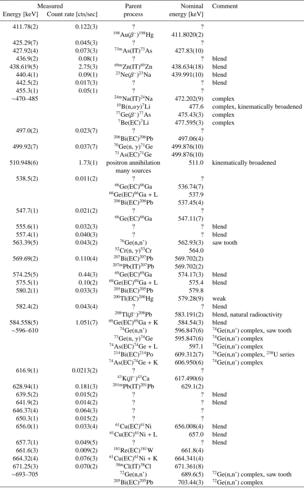
Table 1. continued.
Measured Parent Nominal Comment
Energy [keV] Count rate [cts/sec] process energy [keV]
241.53(3) 0.084(3) 214Pb(β−)214Bi 241.997(3) blend,238U series 55Cr∗ 241.94(5) 253.05(4) 0.063(3) ? ? 257.5(1) 0.021(3) ? ? 234mPa(β−)234U 258.26(10) 238U series 264.64(3) 0.094(3) 77Ge(β−)77As 264.44(3) 77As∗ 264.44(3) 271.257(5) 0.558(5) 44mSc(IT)44Sc 270.9(2) 279.21(1) 0.171(5) 203Pb(EC)203Tl 279.1967(12) 283.2(1) 0.1714(4) ? ? 61Cu(EC)61Ni 282.956(2) 61Cu(EC)61Ni+ L 283.9 291.23(3) 0.070(3) 61Cu(EC)61Ni+ K 291.289(2) complex 295.30(3) 0.112(4) 214Pb(β−)214Bi 295.224(2) complex,238U series 297.40(2) 0.156(4) 73Ga(β−)73Ge 297.32(5) complex 300.24(2) 0.59(1) 67Ga(EC)67mZn 300.219(10) complex
212Pb(β−)212Bi complex,232Th series, weak
301.55(6) 0.144(9) 67Ga(EC)67mZn+ L 301.3 complex 212Pb(β−)212Bi 300.087(10) complex,232Th series 303.87(2) 0.154(5) 75mAs(IT)75As 303.9236(10) complex 309.873(5) 1.207(9) 67Ga(EC)67mZn+ K 309.878(10) blend 311.9(1) 0.060(4) ? ? blend 320.09(2) 0.119(3) 51Cr(EC)51V 320.0824(4) 51Cr(EC)51V+ L 320.7 51Ti(β−)51V 320.0824(4) weak 325.66(1) 0.195(3) 51Cr(EC)51V+ K 325.5475(4) blend 73Ga(β−)73Ge 325.70(7) blend 328.4(1) 0.019(2) ? ? blend 331.14(3) 0.085(3) 201Pb(EC)201Tl 331.19(3) blend 338.22(2) 0.101(3) 228Ac(β−)228Th 338.320(3) 232Th series 343.5(1) 0.019(2) 175Hf(EC)175Lu 343.40(8) 206Bi(EC)206Pb 343.51(3) weak 351.0(1) 0.07(2) 21F(β−)21Ne 350.72(6) blend 352.0(1) 0.17(2) 214Pb(β−)214Bi 351.932(2) blend,238U series 360.6(2) 0.014(2) 181Re(EC)181W 360.7(3) 365.62(3) 0.102(3) 181Re(EC)181W 365.5(3) blend 367.80(5) 0.061(3) 200Tl(EC)200Hg 367.942(10) blend 372.6(3) 0.012(3) 43K(β−)43Ca 372.760(7) blend 43Sc(EC)43Ca 372.760(7) blend 43Sc(EC)43Ca+ L 373.2 blend 374.78(3) 0.095(4) 204Bi(EC)204Pb 374.76(7) blend 204mPb(IT)204Pb 374.76(7) blend 43Sc(EC)43Ca+ L 376.8 blend, weak
381.4(2) 0.012(2) ? ? blend 66Ge(EC)66Ga 381.85(5) blend 383.6(2) 0.016(3) 195Pb(EC)195Tl 383.64(12) blend 195mTl(IT)195Tl 383.64(12) blend 66Ge(EC)66Ga+ L 383.1 blend 390.1(2) 0.017(3) 25Na(β−)25Mg 389.7 complex 392.3(2) 0.07(1) 66Ge(EC)66Ga+ K 392.22(5) complex 393.75(9) 0.210(8) 67Ga(EC)67Zn 393.5(1) complex 67Ga(EC)67Zn+ L 394.6 complex 395.3(1) 0.071(8) ? ? complex 397.98(2) 0.251(3) ? ? complex
206Bi(EC)206Pb 398.00(3) weak, complex
400.47(5) 0.082(3) ? ? complex
G. Weidenspointner et al.: First identification and modelling of SPI background lines, Online Material p 4
Table 1. continued.
Measured Parent Nominal Comment
Energy [keV] Count rate [cts/sec] process energy [keV]
411.78(2) 0.122(3) ? ? 198Au(β−)198Hg 411.8020(2) 425.29(7) 0.045(3) ? ? 427.92(4) 0.073(3) 73mAs(IT)73As 427.83(10) 436.9(2) 0.08(1) ? ? blend 438.619(5) 2.75(3) 69mZn(IT)69Zn 438.634(18) blend 440.4(1) 0.09(1) 23Ne(β−)23Na 439.991(10) blend 442.5(2) 0.017(3) ? ? blend 455.3(1) 0.05(1) ? ? ∼470–485 24mNa(IT)24Na 472.202(9) complex
10B(n,αγ)7Li 477.6 complex, kinematically broadened 77Ge(β−)77As 475.43(3) complex 7Be(EC)7Li 477.595(3) complex 497.0(2) 0.023(7) ? ? 206Bi(EC)206Pb 497.06(4) 499.92(7) 0.037(7) 70Ge(n,γ)71Ge 499.876(10) 71As(EC)71Ge 499.876(10)
510.948(6) 1.73(1) positron annihilation 511.0 kinematically broadened many sources 538.5(2) 0.011(2) ? ? 66Ge(EC)66Ga 536.74(7) 66Ge(EC)66Ga+ L 537.9 206Bi(EC)206Pb 537.45(4) 547.7(1) 0.021(2) ? ? 66Ge(EC)66Ga 547.11(7) 555.6(1) 0.032(3) ? ? blend 557.4(1) 0.040(3) ? ? blend
563.39(5) 0.043(2) 76Ge(n,n’) 562.93(3) saw tooth
52Cr(n,γ)53Cr 564.0 569.69(2) 0.110(4) 207Bi(EC)207Pb 569.702(2) 207mPb(IT)207Pb 569.702(2) 574.25(5) 0.44(3) 69Ge(EC)69Ga 574.17(3) blend 575.5(1) 0.10(2) 69Ge(EC)69Ga+ L 575.4 blend 580.2(1) 0.033(3) 205Bi(EC)205Pb 579.8 200Tl(EC)200Hg 579.28(9) weak 582.4(2) 0.043(4) ? ? blend
208Tl(β−)208Pb 583.191(2) blend, natural radioactivity
584.558(5) 1.051(7) 69Ge(EC)69Ga+ K 584.54(3) blend
∼596–610 74Ge(n,n’) 596.847(6) 74Ge(n,n’) complex, saw tooth 73Ge(n,γ)74Ge 595.847(6) 74Ge(n,n’) complex
74As(EC)74Ge+ L 597.1 74Ge(n,n’) complex
214Bi(EC)214Po 609.312(7) 74Ge(n,n’) complex,238U series 74As(EC)74Ge+ K 606.950(6) 74Ge(n,n’) complex
616.9(1) 0.0213(2) ? ? 43K(β−)43Ca 617.490(6) 628.94(1) 0.181(3) 201mPb(IT)201Pb 629.1(2) 639.5(2) 0.015(2) ? ? blend 641.9(2) 0.014(2) ? ? blend 646.37(4) 0.064(3) ? ? 650.3(1) 0.015(2) ? ? 656.0(1) 0.033(4) 61Cu(EC)61Ni 656.008(4) blend 61Cu(EC)61Ni+ L 657.0 blend 657.7(1) 0.049(5) ? ? blend 661.6(3) 0.009(2) 181Re(EC)181W 661.8(4) 664.32(4) 0.076(3) 61Cu(EC)61Ni+ K 664.341(4) 671.25(3) 0.070(2) 38mCl(IT)38Cl 671.361(8)
∼693–705 72Ge(n,n’) 689.6(5) 72Ge(n,n’) complex, saw tooth 205Bi(EC)205Pb 703.44(3) 72Ge(n,n’) complex
G. Weidenspointner et al.: First identification and modelling of SPI background lines, Online Material p 5
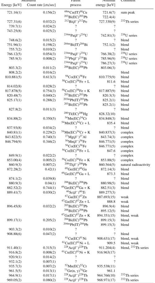
Table 1. continued.
Measured Parent Nominal Comment Energy [keV] Count rate [cts/sec] process energy [keV]
721.16(1) 0.156(2) 68mCu(IT)68Cu 721.6(7) sum peak 203Bi(EC)203Pb 722.4(4) 727.31(6) 0.032(2) 212Bi(β−)212Po 727.330(9) 232Th series 739.7(1) 0.024(2) ? ? 743.25(8) 0.025(2) ? ? 234mPa(β−)234U 742.81(3) 238U series 748.6(2) 0.015(2) ? ? blend 751.96(1) 0.198(2) 204mBi(IT)204Bi 752.1(2) blend 755.7(2) 0.010(2) ? ? blend 766.12(5) 0.054(3) 234mPa(β−)234U 766.38(2) 238U series 785.9(3) 0.008(2) 214Pb(β−)214Bi 785.96(9) 238U series 234mPa(β−)234U 786.27(3) 238U series 803.3(2) 0.011(2) 206Bi(EC)206Pb 803.06(3) 808.2(2) 0.016(2) blend 810.881(5) 0.613(3) 58Co(EC)58Fe 810.775(9) blend 58Co(EC)58Fe+ L 811.6 blend 814.02(8) 0.028(2) ? ? blend 817.878(5) 0.754(3) 58Co(EC)58Fe+ K 817.887(9) blend 820.48(7) 0.040(2) 203Bi(EC)203Pb 820.3(3) blend 825.17(1) 0.288(2) 203mPb(IT)203Pb 825.2(1) blend 203Bi(EC)203Pb 825.2(1) blend 827.8(2) 0.011(3) ? ? blend 200Tl(EC)200Hg 828.32(10) 834.88(2) 0.350(5) 54Mn(EC)54Cr 834.848(3) blend 54Mn(EC)54Cr+ L 835.4 blend 837.93(8) 0.034(2) ? ? blend 840.81(1) 0.229(2) 54Mn(EC)54Cr+ K 840.837(3) complex 843.822(5) 0.740(3) 27Mg(β−)27Al 843.74(3) complex 846.794(9) 0.346(2) 56Mn(β−)56Fe 846.771(5) complex 56Co(EC)56Fe 846.771(5) complex 56Co(EC)56Fe+ L 847.6 complex 849.9(1) 0.022(2) ? ? complex 853.00(4) 0.005(2) 56Co(EC)56Fe+ K 853.88(5) complex 860.9(3) 0.007(2) 208Tl(β−)208Pb 860.564(5) natural radioactivity 872.28(2) 0.42(1) 69Ge(EC)69Ga 872.14(3) blend 69Ge(EC)69Ga+ L 873.3 blend 874.1(2) 0.039(8) ? ? blend 880.9(3) 0.04(1) 206Bi(EC)206Pb 880.98(5) blend 882.52(2) 0.744(1) 69Ge(EC)69Ga+ K 882.51(3) blend 889.41(7) 0.030(2) 46Sc(β−)46Ti 889.277(3) 67Ga(EC)67Zn 887.693(15) weak 67Ga(EC)67Zn+ L 888.8 weak 896.45(8) 0.032(2) 203Bi(EC)203Pb 896.9(4) blend 206Bi(EC)206Pb 895.12(5) blend 67Ga(EC)67Zn+ K 894.351(15) blend, weak
899.17(1) 0.205(2) 204Bi(EC)204Pb 899.15(3) blend 204mPb(IT)204Pb 899.15(3) blend
903.3(2) 0.010(2) ? ? 908.88(6) 0.047(2) ? ? blend
61Cu(EC)61Ni 908.631(17) blend, weak 61Cu(EC)61Ni+ L 909.5 blend, weak
911.40(1) 0.315(3) 228Ac(β−)228Th 911.204(4) blend,232Th series 916.8(2) 0.008(2) 61Cu(EC)61Ni+ K 916.963(17) 920.9(1) 0.014(2) ? ? 932.1(2) 0.007(1) ? ? 935.7(3) 0.007(2) 52Mn(EC)52Cr 935.538(11) 961.5(5) 0.013(1) 73Ge(n,γ)74Ge 961.1 964.9(1) 0.017(1) 228Ac(β−)228Th 964.766(10) 232Th series 969.05(2) 0.080(2) 228Ac(β−)228Th 968.971(17) 232Th series
G. Weidenspointner et al.: First identification and modelling of SPI background lines, Online Material p 6
Table 1. continued.
Measured Parent Nominal Comment Energy [keV] Count rate [cts/sec] process energy [keV]
974.85(7) 0.0243(1) 25Na(β−)25Mg 974.72 983.80(3) 0.064(2) 48V(EC)48Ti 983.517(5) blend 48Sc(β−)48Ti 983.517(5) blend 48V(EC)48Ti+ L 984.2 blend 204Bi(EC)204Pb 983.98(3) blend 987.595(6) 0.384(2) 205mPb(IT)205Pb 987.62(3) blend 48V(EC)48Ti+ K 988.702(5) blend 991.96(6) 0.029(2) ? ? 1001.14(2) 0.068(2) 234mPa(β−)234U 1001.03(3) 238U series 1014.485(7) 0.283(2) 27Mg(β−)27Al 1014.42(3) 205mPb(IT)205Pb 1013.84(3) 1021.96(3) 0.067(2) positron annihilation 1022.0 many sources 1026.3(1) 0.013(1) ? ? 1037.9(4) 0.010(4) 48Sc(β−)48Ti 1037.599(26) blend 1039.49(7) 0.057(4) 66Ga(EC)66Zn 1039.237(3) blend
70Ge(n,n’) 1039.20(8) blend, saw tooth 66Ga(EC)66Zn+ L 1040.3 blend 1044.4(2) 0.009(2) ? ? 1048.94(5) 0.040(2) 66Ga(EC)66Zn+ K 1048.896(3) 1063.75(3) 0.067(2) 207mPb(IT)207Pb 1063.662(4) 1077.59(3) 0.062(2) 68Ga(EC)68Zn 1077.34(5) 68Ga(EC)68Zn+ L 1078.4 1087.09(2) 0.097(2) 68Ga(EC)68Zn+ K 1087.00(5) 1095.7(3) 0.006(1) ? ? 1106.98(3) 0.92(4) 69Ge(EC)69Ga 1107.01(6) blend 1108.36(7) 0.17(3) 69Ge(EC)69Ga+ L 1108.2 blend 1115.46(2) 0.353(8) 65Zn(EC)65Cu 1115.546(4) blend 65Zn(EC)65Cu+ L 1116.5 blend 1117.257(6) 1.79(1) 69Ge(EC)69Ga+ K 1117.38(6) blend
1120.87(2) 0.112(3) 214Bi(EC)214Po 1120.287(10) blend,238U series
46Sc(β−)46Ti 1120.545(4) blend 182Ta(β−)182W 1121.3008(17) blend 1124.513(4) 0.545(3) 65Zn(EC)65Cu+ K 1124.525(4) 1139.3(2) 0.011(1) ? ? 1157.08(7) 0.024(1) 44Sc(EC)44Ca 1157.020(15) 1161.2(2) 0.009(1) ? ? 1172.9(2) 0.009(1) 60Co(β−)60Ni 1173.228(3) 1185.6(2) 0.009(1) 61Cu(EC)61Ni 1185.234(15) 61Cu(EC)61Ni+ L 1186.2 1189.40(6) 0.031(1) 182Ta(β−)182W 1189.0503(17) 205Bi(EC)205Pb 1190.03(4) 1193.6(1) 0.018(1) 61Cu(EC)61Ni+ K 1193.57(2) 1204.7(1) 0.014(1) 73Ge(n,γ)74Ge 1204.2 200Tl(EC)200Hg 1205.70(9) 1221.45(4) 0.039(1) 182Ta(β−)182W 1221.4066(17) 1231.0(2) 0.011(1) 182Ta(β−)182W 1231.0156(17) 1238.4(1) 0.015(1) 214Bi(β−)214Po 1238.11(1) 238U series 56Co(EC)56Fe 1238.282(7) weak 201Pb(EC)201Tl 1238.76(7) weak 1274.05(9) 0.027(1) ? ? blend 22Na(EC)22Ne 1274.53(2) blend 1276.8(5) 0.004(1) 201Pb(EC)201Tl 1277.13(7) blend 1290.8(3) 0.008(1) ? ? blend 1293.4(1) 0.024(2) 41Ar(β−)41K 1293.64(4) blend 1298.63(8) 0.019(1) ? ? 1312.10(7) 0.022(1) 48V(EC)48Ti 1312.096(6) 48Sc(β−)48Ti 1312.096(6) 48V(EC)48Ti+ L 1312.6
G. Weidenspointner et al.: First identification and modelling of SPI background lines, Online Material p 7
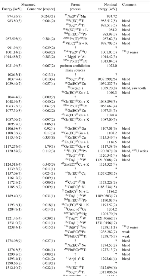
Table 1. continued.
Measured Parent Nominal Comment
Energy [keV] Count rate [cts/sec] process energy [keV]
1316.6(3) 0.005(1) ? ? 48V(EC)48Ti+ K 1317.062(6) 1332.5(1) 0.013(1) 60Co(β−)60Ni 1332.492(4) 1336.82(2) 0.109(2) 69Ge(EC)69Ga 1347.09(6) 69Ge(EC)69Ga+ L 1348.3 ? ? 1345.4(4) 0.017(8) ? ? blend 1347.04(6) 0.147(9) 69Ge(EC)69Ga+ K 1347.09(6) blend 1354.2(4) 0.005(1) ? ? 1357.0(3) 0.006(1) ? ? 1364.4(2) 0.008(1) ? ? 1368.650(9) 0.201(2) 24Na(β−)24Mg 1368.626(5) 1377.89(6) 0.033(1) 214Bi(β−)214Po 1377.669(12) 238U series 1381.79(3) 0.064(2) 48Ti(n,γ)49Ti 1381.745(4) 1394.6(6) 0.003(1) 21F(β−)21Ne 1395.131(17) 1397.7(4) 0.005(1) ? ? 1408.1(3) 0.005(1) 214Bi(β−)214Po 1407.98(4) 238U series 1434.15(2) 0.072(1) 52V(β−)52Cr 1434.068(14) PSD 52Mn(EC)52Cr 1434.068(14) PSD, weak
1460.80(2) 0.114(2) 40K(EC)40Ar 1460.822(6) PSD, natural radioactivity
1481.1(3) 0.005(1) ? ? PSD 1497.7(3) 0.005(1) ? ? PSD, blend 1501.5(2) 0.006(1) ? ? PSD, blend 1525.5(1) 0.0132(9) 69Ge(EC)69Ga 1525.83(7) PSD 69Ge(EC)69Ga+ L 1527.0 PSD 1536.33(4) 0.035(1) 69Ge(EC)69Ga+ K 1536.20(7) PSD 203Bi(EC)203Pb 1536.4(4) PSD 1552.1(2) 0.012(1) ? ? PSD 1580.4(3) 0.007(1) ? ? PSD, blend 1587.5(1) 0.024(1) ? ? PSD, blend 1609.1(2) 0.018(1) ? ? PSD, blend 1613.1(1) 0.029(2) 56Fe(n,γ)57Fe 1612.8 PSD, blend 1620.7(2) 0.009(1) 212Bi(β−)212Po 1620.5(1) PSD 1630.9(2) 0.013(1) ? ? PSD, blend 1633.66(3) 0.123(3) 20Ne∗ 1633.602(15) PSD, blend 20F(β−)20Ne 1633.602(15) PSD 1648.3(4) 0.004(1) ? ? 1658.4(1) 0.014(1) ? ? ∼1670–1700 58Co(EC)58Fe 1674.730(10) complex 58Co(EC)58Fe+ L 1675.5 complex 58Co(EC)58Fe+ K 1681.843(10) complex 1719.0(2) 0.005(1) 206Bi(EC)206Pb 1718.70(7) 203Bi(EC)203Pb 1719.7(4) 1724.9(2) 0.005(1) 56Fe(n,γ)57Fe 1725.09(6) 1729.5(1) 0.0087(7) ? ? 1758.3(3) 0.005(1) ? ? 1764.34(2) 0.222(4) 205Bi(EC)205Pb 1764.36(4) 214Bi(β−)214Po 1764.494(14) 238U series 1776.00(7) 0.039(2) 205Bi(EC)205Pb 1775.79(4) blend 1778.961(8) 0.365(4) 28Al(β−)28Si 1778.969(12) blend 1805.8(3) 0.007(1) ? ? blend 1808.7(1) 0.029(2) 26Na(β−)26Mg 1808.66(3) blend 26Mg∗ 1808.66(3) blend 1810.9(2) 0.017(2) 56Mn(β−)56Fe 1810.772(17) blend 1832.3(1) 0.007(1) ? ? 1847.4(2) 0.0072(7) 203Bi(EC)203Pb 1847.4(3) 214Bi(β−)214Po 1847.42(3) 238U series 1861.7(2) 0.005(1) ? ?
G. Weidenspointner et al.: First identification and modelling of SPI background lines, Online Material p 8
Table 1. continued.
Measured Parent Nominal Comment
Energy [keV] Count rate [cts/sec] process energy [keV]
1882.5(2) 0.007(1) 66Ga(EC)66Zn+ K 1882.440(3) sum peak
? ? 1888.0(2) 0.0087(7) 203Bi(EC)203Pb 1888.2(3) blend 1892.37(9) 0.0176(8) 69Ge(EC)69Ga 1891.55(7) blend 69Ge(EC)69Ga+ L 1892.8 blend 203Bi(EC)203Pb 1893.0(3) blend 1901.85(9) 0.0170(9) 69Ge(EC)69Ga+ K 1901.92(7) 1919.8(3) 0.005(1) ? ? 1923.8(4) 0.0051(8) 69Ge(EC)69Ga 1923.8(2) 69Ge(EC)69Ga+ L 1925.0 1927.5(4) 0.004(1) ? ? 1934.13(9) 0.0140(8) 69Ge(EC)69Ga+ K 1934.2(2) 1940.9(3) 0.004(1) ? ? 1964.9(2) 0.005(1) ? ? 2011.6(6) 0.0023(8) ? ? 203Bi(EC)203Pb 2011.4(6) 2024.00(1) 0.013(1) 69Ge(EC)69Ga 2023.99(13) 69Ge(EC)69Ga+ L 2025.2 2033.95(9) 0.017(1) 69Ge(EC)69Ga+ K 2034.36(13) 2113.0(2) 0.0068(7) 56Mn(β−)56Fe 2113.123(10) 2117.7(5) 0.0022(6) ? ? 2167.3(3) 0.0039(7) ? ?
∼2195–2223 214Bi(β−)214Po 2204.21(4) complex,238U series
27Al∗ 2211.0(7) complex, kinematically broadened
2223.42(2) 0.1086(9) 1H(n,γ)2D 2223.255(4) complex
2236.8(2) 0.0052(6) ? ?
2295.5(4) 0.0035(6) 48V(EC)48Ti 2295.625(7) blend, sum peak 48V(EC)48Ti+ L 2296.1 blend, sum peak
2300.7(1) 0.0112(7) 48V(EC)48Ti+ K 2300.591(4) blend, sum peak
2319.1(1) 0.0153(7) ? ? 2390.6(2) 0.0052(5) ? ? 2448.0(3) 0.0036(5) ? ? 2507.1(3) 0.0042(5) ? ? 2512.8(4) 0.0031(5) ? ? 2528.5(4) 0.0027(5) ? ? 2599.5(3) 0.0039(5) ? ? 2614.61(3) 0.0380(6) 208Tl(β−)208Pb 2614.533(13) natural radioactivity 2657.3(3) 0.0031(5) 56Mn(β−)56Fe 2657.45(5) 2741.7(3) 0.0037(4) ? ? 2749.9(2) 0.0120(9) ? ? blend 66Ga(EC)66Zn 2751.852(6) blend 66Ga(EC)66Zn+ L 2753.0 blend 2754.03(1) 0.153(1) 24Na(β−)24Mg 2754.01(1) blend 2761.4(1) 0.0082(4) 66Ga(EC)66Zn+ K 2761.511(6) 2959.5(5) 0.0048(6) ? ? 2982.0(7) 0.0028(5) ? ?
∼2993–3013 27Al∗ 3004.3 complex, kinematically broadened
3034.2(6) 0.0032(5) ? ? 3120.0(3) 0.0018(4) ? ? 3229.1(2) 0.0040(3) 66Ga(EC)66Zn 3228.824(9) 66Ga(EC)66Zn+ L 3229.9 48V(EC)48Ti+ K 3228.858(11) 3238.2(1) 0.0066(4) 66Ga(EC)66Zn+ K 3238.483(6) 3381.2(2) 0.0046(4) 66Ga(EC)66Zn 3380.88(1) 66Ga(EC)66Zn+ L 3381.2 3390.2(2) 0.0037(3) 66Ga(EC)66Zn+ K 3390.54(1) 3451.7(5) 0.0013(3) 56Co(EC)56Fe 3451.152(17)
G. Weidenspointner et al.: First identification and modelling of SPI background lines, Online Material p 9
Table 1. continued.
Measured Parent Nominal Comment
Energy [keV] Count rate [cts/sec] process energy [keV] 3791.4(1) 0.0085(3) 66Ga(EC)66Zn 3791.036(8) 66Ga(EC)66Zn+ L 3792.1 3800.26(4) 0.0220(4) 66Ga(EC)66Zn+ K 3800.695(8) 3852.4(5) 0.0015(3) 13C∗ 3853.170(22) 4085.8(2) 0.0045(3) 66Ga(EC)66Zn 4085.875(12) 66Ga(EC)66Zn+ L 4087.0 4095.4(2) 0.0048(3) 66Ga(EC)66Zn+ K 4095.543(12)
4122.14(7) 0.0105(3) 24Na(β−)24Mg 4122.633(12) sum peak
4295.27(7) 0.0137(4) 66Ga(EC)66Zn 4295.224(10) 66Ga(EC)66Zn+ L 4296.3
4304.54(6) 0.0151(3) 66Ga(EC)66Zn+ K 4304.883(10)
4434.(3.) 0.021(2) 12C∗ 4438.03(31) kinematically broadened, FWHM∼90 keV
4461.1(2) 0.0035(3) 66Ga(EC)66Zn 4461.247(13) 66Ga(EC)66Zn+ L 4462.3 4470.6(2) 0.0030(2) 66Ga(EC)66Zn+ K 4470.906(13) 4805.9(1) 0.0057(3) 66Ga(EC)66Zn 4806.060(18) 66Ga(EC)66Zn+ L 4807.2 4815.2(1) 0.0061(3) 66Ga(EC)66Zn+ K 4815.719(18) 4881.9(4) 0.0009(2) ? ? 5269.1(3) 0.0017(2) 15N∗ 5269.161(14) 5297.7(4) 0.0016(2) 15C(β−)15N 5297.817(14) 5450.7(4) 0.0013(2) ? ? 5518.0(4) 0.0024(3) 72Ge(n,γ)73Ge 5518.3 5529.(1.) 0.0010(2) ? ? 5618.1(2) 0.0037(3) 52Cr(n,γ)53Cr 5618.2 16O∗ ∼5617.6 single escape 16N(β−)16O ∼5617.6 single escape 5910.8(2) 0.0056(3) ? ? 5920.2(4) 0.0021(2) 56Fe(n,γ)57Fe 5920.45(2)
5994.6(4) 0.0014(2) 74Ge(n,γ)75Ge ∼5994.1 single escape
6018.9(5) 0.0011(2) 56Fe(n,γ)57Fe 6018.4 6036.7(6) 0.0009(2) ? ? ∼6105–6129 70Ge(n,γ)71Ge 6116.9 complex 6128.94(4) 0.0283(4) 16O∗ 6128.63(4) 16N(β−)16O 6128.63(4) 6204.5(4) 0.0018(2) ? ?
72Ge(n,γ)73Ge ∼6206.0 single escape
6250.7(2) 0.0043(2) ? ?
48Ti(n,γ)49Ti ∼6249.1 single escape
6276.1(7) 0.0012(2) ? ? 6320.2(5) 0.0015(2) ? ? 6365.1(3) 0.0025(2) 74Ge(n,γ)75mGe 6365.4 S n− 139.69 keV 6391.7(4) 0.0018(2) ? ? 72Ge(n,γ)73Ge 6390.2
70Ge(n,γ)71Ge ∼6393.6 double escape
6418.0(1) 0.0063(3) 72Ge(n,γ)73Ge 6418.6 48Ti(n,γ)49Ti 6418.4 6499.6(6) 0.0023(4) ? ? blend 6505.3(1) 0.0153(4) 74Ge(n,γ)75Ge 6505.1 blend, S n 6556.2(5) 0.0015(2) 48Ti(n,γ)49Ti 6555.9 6707.7(3) 0.0037(3) 70Ge(n,γ)71Ge 6707.5 blend 6716.1(1) 0.0155(5) ? ? blend 72Ge(n,γ)73Ge 6717.0 blend 6753.9(5) 0.0023(3) ? ? blend 6760.3(1) 0.0164(4) 48Ti(n,γ)49Ti 6760.1 blend 6770.9(6) 0.0012(2) ? ? blend 6781.5(3) 0.0025(2) ? ? blend 6809.8(1) 0.0049(2) 9Be(n,γ)10Be 6809.9 S n
G. Weidenspointner et al.: First identification and modelling of SPI background lines, Online Material p 10
Table 1. continued.
Measured Parent Nominal Comment
Energy [keV] Count rate [cts/sec] process energy [keV] 6837.7(3) 0.0025(2) 62Ni(n,γ)63Ni 6837.4
6904.5(3) 0.0035(2) 70Ge(n,γ)71Ge ∼6904.6 single escape
6915.6(5) 0.0014(2) 70Ge(n,γ)71Ge 6915.7
7119.5(2) 0.0063(3) 56Fe(n,γ)57Fe ∼7120.2 single escape
7134.3(3) 0.0041(2) 56Fe(n,γ)57Fe ∼7134.6 single escape
7159.9(9) 0.0012(2) ? ?
7214.5(3) 0.0036(3) 27Al(n,γ)28Al ∼7212.9 single escape 70Ge(n,γ)71Ge 7217.2 S n− 198.4 keV 7243.4(4) 0.0026(3) 55Mn(n,γ)56Mn 7243.4 7276.7(6) 0.0018(2) ? ? 56Fe(n,γ)57Fe 7278.8 7306.8(8) 0.0013(2) 63Cu(n,γ)64Cu 7307.3
∼7400-7415 63Cu(n,γ)64Cu ∼7405.3 complex, single escape
7415.66(6) 0.0307(5) 70Ge(n,γ)71Ge 7415.6 complex, S ncascade 7426.9(5) 0.0014(2) 52Cr(n,γ)53Cr ∼7427.6 single escape 7623.3(4) 0.0031(3) ? ? blend 7631.5(1) 0.0228(4) 56Fe(n,γ)57Fe 7631.2 blend 7645.7(1) 0.0188(4) 56Fe(n,γ)57Fe 7645.6 S n 7694.1(5) 0.0013(2) 27Al(n,γ)28Al 7693.4 7716.0(9) 0.0011(2) ? ? blend 7724.4(1) 0.0112(3) 27Al(n,γ)28Al 7724.0 blend, S n 7819.0(4) 0.0014(2) 60Ni(n,γ)61Ni 7819.4 7910.5(4) 0.0025(3) ? ? blend 7915.7(1) 0.0100(3) 63Cu(n,γ)64Cu 7916.3 blend, S n 7939.3(3) 0.0023(2) 52Cr(n,γ)53Cr 7938.6
8488.(1.) 0.0011(2) 58Ni(n,γ)59Ni ∼8487.4 multiple, single escape
8578.(1.) 0.0011(2) ? ? multiple
8998.0(4) 0.0027(3) 58Ni(n,γ)59Ni 8998.4 multiple, S
n 9598.3(9) 0.0006(1) 73Ge(n,γ)74Ge 9600.2 multiple, S
n− 595.8 keV 9683.6(9) 0.0006(1) 73Ge(n,γ)74Ge ∼9685.2 multiple, single escape
10195.0(4) 0.0057(3) 73Ge(n,γ)74Ge 10196.2 multiple, S
n
The meaning of standardized comments in Col. 5 is as follows:
– blend: a line-like feature consisting of a few components that blend because they are closely spaced in energy; resolving the components can
be very difficult and systematic uncertainties can be much larger than the quoted statistical errors.
– complex: a complex spectral feature which can result from the blending of many lines, from the presence of a single broad structure, or both;
sometimes the complex is named for its dominant component.
– weak: indicates a contribution to a line that is expected to be significantly weaker than all other contributions. – sum peak: the peak results from the coincident interaction of two gamma rays from the same de-excitation cascade.
– natural radioactivity: the parent isotope is so-called “naturally” radioactive, i.e. it is not radioactive because of activation processes in orbit. – . . . series: similar to above, except that the parent isotope is a member of the quoted so-called natural decay series.
– saw tooth: a saw tooth or triangular shaped spectral feature due to inelastic neutron scattering in the Ge detector, the saw tooth results from
the summation of the gamma-ray energy and the recoil energy of the excited Ge nucleus.
– PSD: the line rate has been corrected for the efficiency of the PSD electronics. – single/double escape: single/double escape peak.
– multiple: the line occurs only in multiple event data, the quoted rate is for the sum of double and triple events.
– Sn: when a thermal neutron is captured, the excitation energy of the product nucleus is equal to its neutron separation energy Sn; in the table