Development of a Hybrid Deterministic-Stochastic Method for Full Core Neutronics

(1)

DEVELOPMENT OF A HYBRID DETERMINISTIC - STOCHASTIC METHOD FOR FULL CORE NEUTRONICS

SEYED RIDA HOUSSEINY MILANY DÉPARTEMENT DE GÉNIE PHYSIQUE ÉCOLE POLYTECHNIQUE DE MONTRÉAL

THÈSE PRÉSENTÉE EN VUE DE L’OBTENTION DU DIPLÔME DE PHILOSOPHIÆ DOCTOR

(GÉNIE NUCLÉAIRE) FÉVRIER 2017

c

(2)

ÉCOLE POLYTECHNIQUE DE MONTRÉAL

Cette thèse intitulée:

DEVELOPMENT OF A HYBRID DETERMINISTIC - STOCHASTIC METHOD FOR FULL CORE NEUTRONICS

présentée par: HOUSSEINY MILANY Seyed Rida

en vue de l’obtention du diplôme de: Philosophiæ Doctor a été dûment acceptée par le jury d’examen constitué de:

M. TEYSSEDOU Alberto, Ph. D., président

M. MARLEAU Guy, Ph. D., membre et directeur de recherche M. KOCLAS Jean, Ph. D., membre

(3)

DEDICATION

To the one who leads me through the routes of life and to my father ...

(4)

ACKNOWLEDGEMENTS

The work presented in this thesis has been partly funded through a research grant from the Natural Sciences and Engineering Research Council of Canada. The financial support I received through the duration of the project is acknowledged.

This research project has been carried under close supervision by professor Guy Marleau. His feedback, comments and input has helped greatly shape the work since the initiation point up to accomplishment. Professor Marleau is acknowledged for granting me the opportunity to complete my PhD research under his supervision and for his close mentorship and support. As this thesis marks the end of my academic journey, I would like to express my gratitude and thankfulness to every tutor and teacher that taught me a single word throughout my education. Professor Malcolm Joyce from Lancaster University is especially acknowledged for encouraging me to pursue a research path towards a PhD and for securing me a research grant to complete my Master degree that was a key point in my education.

Professor Seyed Fadhel Milany is always acknowledged for his continuous support and en-couragement during my higher education.

Finally, my family are always thanked and acknowledged for their limitless care and love. Achieving this work would’nt have been possible without their encouragement and love.

(5)

RÉSUMÉ

La conception, l’analyse et le fonctionnement des réacteurs de fission nucléaire dépendent de la compréhension des vitesses des différentes réactions neutroniques dans le cœur du réacteur. C’est pour cela que la distribution du flux neutronique dans le cœur doit être estimée avec une bonne précision. Depuis la découverte de la fission nucléaire et l’introduction des réacteurs nucléaires, différentes approches déterministes et stochastiques ont été développées ayant pour but la modélisation des cœurs du réacteur ainsi que l’étude de la distribution du flux des neutrons. Les méthodes neutroniques actuelles utilisées pour simuler des réacteurs complets souffrent d’une précision relativement faible ou nécessitent des ressources en mémoire et en temps de calcul extrêmes. La conception de nouvaux réacteurs nucléaires demande de nouvelles méthodes qui soient à la fois précises et pratiques dans les applications de production pour la simulation et l’étude de la neutronique.

Dans ce travail, une revue de la méthode Monte Carlo (MC) et de ses défis est incluse. La méthode MC est basée sur le suivi statistique des neutrons basés sur des distributions de probabilité physique qui le rend très proche d’un réacteur virtuel. La solution qu’elle fournit est largement acceptée comme une estimation précise de la distribution du flux neutronique bien que les coûts de calculs soient importants. Dans les études MC de cœur complet, un grand nombre de paramètres physiques sont enregistrés et la taille de l’échantillon statistique doit être très grande pour obtenir une solution avec une confiance élevée. L’extrême charge de calcul des simulations de cœur complet basées sur MC son utilisation pour des calculs de production peu pratiques et la méthode a été limitée pour l’étalonnage et la validation. La convergence lente de la source de fission, la difficulté de la coupler aux solveurs de rétroaction multiphysique et l’estimation de la variance vraie sont d’autres défis pour les études MC de cœur.

L’utilisation des méthodes déterministes s’avère donc inévitables. Ces dernières sont basées sur la discrétisation de l’équation du transport dans l’espace de phase. Ces méthodes sont également fondées sur l’obtention d’une solution approximative à l’aide des méthodes numériques. Ici, un résumé de l’étude de l’équation de transport et de l’approximation des probabilités de collision est présenté. En plus de la solution du mode fondamental décrivant la répartition asymptotique du flux neutronique, l’équation de transport suppose un grand nom-bre de solutions qui peuvent être très utiles dans les études de la perturbation, la cartographie et la synthèse des flux neutroniques. Les méthodes de calcul impliquant des solutions bien ordonnées de l’équation de transport telles que la déflation et la décomposition QZ ont été

(6)

ex-aminées. Celles-ci sont appliquées à un certain nombre de problèmes, dans le but d’effectuer une comparaison entre eux. On observe que la déflation souffre d’une convergence médiocre et de long temps de calcul, alors que la méthode QZ assure la convergence des solutions pour les modes d’ordre élevé durant un temps raisonnable. L’application des modes dominants de l’équation de transport à la cartographie du flux a été décrite. Ainsi, la reconstruction d’une solution de transport sur un maillage spatial fin, telle que la solution de la diffusion homogène a été présentée.

Afin de remédier aux dépenses extrêmes des simulations MC, nous proposons ici une approche hybride basée sur la combinaison des solveurs conventionnels MC et de la cartographie du flux déterministe. Premièrement, nous avons réalisé une simulation stochastique pour produire des flux de neutrons dans quelques régions, ou sur un réseau grossier, ainsi qu’en utilisant des sections efficaces neutroniques homogénéisées et condensées. Les sections efficaces sont util-isées pour un calcul de réseau déterministe afin d’obtenir les modes dominants de l’équation de transport. Une fois les modes dominants calculés, et dans le but d’estimer les amplitudes des modes et effectuer la synthèse du flux pour obtenir une distribution de flux complète, ces modes seront combinés aux solution du solveur MC. Deux approches sont envisagées pour réduire la charge de calcul des simulations MC. La première approche consiste à compter quelques régions du réacteur et reconstruire de façon précise une distribution plus détaillée du flux neutronique en utilisant les modes dominants de l’équation de transport et de la car-tographie des flux. Alternativement, les solutions MC sont évaluée sur un maillage grossier et la reconstruction du flux est obtenue en utilisant des modes dominants calculés sur un maillage fin. Ce dernier est plus efficace car une réduction du nombre d’enregistrements et d’histoires de neutrons est réalisable.

Nous avons également évalué la précision de la reconstruction d’une solution MC en utilisant des modes dominants de l’équation de transport et du flux neutronique. La possibilité de reconstruire une distribution du flux neutronique basée sur l’évaluation du flux dans quelques régions a été étudiée et montre la faisabilité de cette méthode. En se basant sur les résultats obtenus, l’étude confirme que l’approche hybride est capable de reconstituer une distribution de flux MC à partir de données de flux dans quelques régions. Par conséquent, une réduction considérable de la dépense de calcul est réalisable.

Pour une meilleure performance, la méthode hybride est développée pour reconstruire une solution à mailles fines à partir d’une solution MC à mailles grossières en utilisant les modes dominants de l’équation de transport. La méthode est appliquée à un certain nombre de problèmes 2D et 3D et la précision et la performance de calcul sont évaluées. Les résultats confirment que dans une simulation de cœur complet, l’approche hybride pourrait être jusqu’à

(7)

90% plus rapide que le methode conventionnelle tout en maintenant une précision comparable. Les solutions produites par la méthode hybride pour les exemples étudiés sont comparées à une référence MC. Dans la plupart des cas, la différence relative entre la solution hybride et la référence est inférieure à 2%, tandis que des erreurs jusqu’à 5% sont observées dans quelques cas. Enfin, les effets du le l’évolution du combustible sont évalués et il est conclu que la méthode peut être utilisée pour des simulations dynamiques à condition que les modes dominants soient recalculés à la fin de chaque étape de combustion.

Le travail présenté dans ce projet de recherche sert de preuve du concept essentiel de la méth-ode hybride. Néanmoins, cette nouvelle méthméth-ode présente quelques limitations et quelques points faibles. Ces limitations devraient être étudiées dans le futur.

Durant ce travail, pour tous les exemples étudiés, la méthode hybride a été appliquée pour l’étude du flux de neutron à deux groupes d’énergie. Le temps de calcul pour obtenir les modes dominants de l’équation de transport dans un maillage spatial fin constitue 16% du temps de calcul de la méthode hybride. Ce temps devrait augmenter significativement avec l’augmentation des nombres des groupes d’énergie. De plus, la demande de mémoire pour le calcul des modes dominants sera relativement importante lorsqu’une structure de groupe plus détaillée ou un maillage spatial plus fin sont utilisés. L’augmentation du temps de calcul et de l’espace mémoire demandé, pourraient contrebalancer les économies réalisées en utilisant cette méthode. Par conséquent, nous pouvons déduire que la méthode hybride est limitée aux problèmes à quelques groupes d’énergie.

Les effets de plusieurs facteurs tels que le nombre de modes dominants utilisés dans l’expansion modale, les effets des conditions aux limites et l’estimation des erreurs sont aussi étudiés. Dans les exemples considérés, différents nombres de modes ont été utilisés pour la cartogra-phie du flux. Une comparaison entre les résultats montre que la précision de la solution reconstruite est légèrement sensible au nombre de modes utilisés dans le modèle d’expansion modale. Il semble que l’augmentation du nombre de modes ne garantit pas une meilleure solution par rapport aux cas où peu de modes sont utilisés. Une stratégie pour sélectionner le nombre de modes dans la synthèse de flux n’est pas décidée dans ce travail et doit être développée. Ces critères pourraient être l’utilisation de modes ayant des valeurs propres non nulles ou de valeurs propres supérieures à un seuil prédéterminé.

L’introduction de conditions aux frontières entraîne des erreurs relativement importantes, près des frontières ou des interfaces. Les résultats confirment que les conditions aux frontières utilisées dans le calcul des modes dominants ont une influence importante sur la précision de la solution. La prise en compte des effets interfaciaux dans le solveur déterministe améliore la précision de la solution. L’utilisation d’une approche par essais et erreurs pour définir

(8)

les conditions aux limites d’albédo confirme que l’inclusion des effets d’interface dans le solveur déterministe améliore la précision de la solution près des interfaces. Cependant, une approche par essais et erreurs n’est pas pratique. Alors, pour déterminer les conditions limites optimales dans le calcul des modes dominants, une autre méthode doit être développée. Une approche possiblement utile est de définir les conditions aux limites d’albedo en utilisant les courants aux les interfaces comptées par le solveur stochastique. Dans les problèmes 3D présentant des conditions aux limites des fuites dans la direction axiale, la précision de la reconstruction de flux avec des modes 2D est moins précise dans les plans proches des frontières. Ceci met en évidence les effets des fuites axiales et la nécessité de les comptabiliser dans le calcul des modes et pour la cartographie des flux.

Une tentative d’estimation de l’erreur de reconstruction des flux est proposée. La méthode semble être utile pour éliminer ou réduire la sensibilité de l’approche hybride au nombre de modes dominants. Néanmoins, la méthode d’estimation d’erreur ne réussit pas à estimer ou à réduire ces erreurs de reconstruction. Par conséquent, une meilleure approche pour l’évaluation des erreurs de cartographie est nécessaire. A partir des problèmes présentés dans le cas des combustibles homogénéisés, on déduit que cette erreur est liée à l’absorption des neutrons. Il serait intéressant de developer une approche similaire pour affronter des problèmes hétérogènes de maille fine.

Enfin, la méthode hybride décrite dans ce travail utilise la méthode de décomposition QZ avec l’approximation de probabilité de collision isotrope pour calculer les modes dominants de l’équation de transport. L’approche QZ peut être très exigeante sur le plan informatique. Toutefois, afin de résoudre des problèmes de valeurs propres, d’autres méthodes numériques doivent être étudiées. Le calcul des modes dominants de l’équation de transport à partir de modèles alternatifs tels que des ordonnées discrètes ou des caractéristiques doit être considéré.

(9)

ABSTRACT

Research efforts in reactor physics focus on the improvement of current analysis methods for neutronics or development of advanced ones. Recently, there is a renewed interest in stochas-tic simulations due to their superior accuracy and the advances in computing platforms. In particular, there is an interest in the development of hybrid stochastic deterministic meth-ods for accelerating the inactive cycles of Monte Carlo. However, such hybrid approaches are not very efficient as the inactive cycle constitute a very small portion of the simulation. In this work, a novel hybrid method is developed and discussed. The approach combines conventional Monte Carlo with deterministic flux mapping to reduce computational costs of full core simulations. The main contributors to the computational expenses of Monte Carlo is the number of tallies scored and the number of neutron histories tracked. In the proposed hybrid method, the Monte Carlo simulation is performed with a small number of neutron histories while maintaining good confidence and scoring flux tallies on a coarse mesh. Then, the dominant modes of the transport equation and flux mapping are employed to reconstruct the neutron flux and reaction rates on a finer mesh. Application to a number of exam-ple problems show that the studied hybrid method can achieve up to 90% reduction in the computational time compared to conventional Monte Carlo while maintaining comparable accuracy.

(10)

TABLE OF CONTENTS DEDICATION . . . iii ACKNOWLEDGEMENTS . . . iv RÉSUMÉ . . . v ABSTRACT . . . ix TABLE OF CONTENTS . . . x

LIST OF TABLES . . . xiii

LISTE OF FIGURES . . . xiv

CHAPTER 1 INTRODUCTION . . . 1

1.1 Problem Formulation . . . 2

1.2 Research Definition and Aims . . . 2

1.3 Thesis Structure . . . 3

CHAPTER 2 LITERATURE REVIEW . . . 4

2.1 The Monte Carlo Method . . . 4

2.2 Challenges for Full Core Monte Carlo . . . 6

2.2.1 Accounting for Multiphysics Feedback . . . 6

2.2.2 Computational Time . . . 7

2.2.3 Memory Demand . . . 7

2.2.4 Convergence of the Fission Source . . . 8

2.2.5 Variance Estimation . . . 12

2.3 Global Acceleration Techniques . . . 12

2.4 Full-Core MC Codes . . . 14

2.4.1 MC21 . . . 15

2.4.2 McCARD . . . 17

2.4.3 Serpent . . . 18

2.4.4 OpenMC . . . 19

CHAPTER 3 THE TRANSPORT EQUATION AND ITS SOLUTIONS . . . 21

(11)

3.2 The Collision Probability Method . . . 22

3.3 High Order Modes of the Transport Equation . . . 24

3.3.1 QZ Decomposition . . . 24

3.3.2 Inverse Power Iteration with Deflation . . . 33

3.4 Flux Mapping using the High Order Modes . . . 35

3.5 Summary . . . 42

CHAPTER 4 FEASIBILITY STUDY . . . 43

4.1 The Hybrid Method . . . 43

4.2 MC Solution Reconstruction Using Dominant Modes . . . 44

4.2.1 MC vs. Fundamental Mode . . . 45

4.2.2 MC Flux Reconstruction Using the Most Dominant Modes . . . 47

4.2.3 Mapping Optimisation and Error Reduction . . . 51

4.3 MC Flux Reconstruction Using Few Tallies . . . 57

4.3.1 Iteratively Re-weighted Least Square . . . 61

4.3.2 Tally Selection Procedure . . . 67

4.4 Summary . . . 72

CHAPTER 5 PRACTICAL IMPLEMENTATION AND APPLICATION . . . 73

5.1 Improved Hybrid Method . . . 73

5.2 Application to Single Fuel Assembly . . . 75

5.2.1 Cross Sections Generation and Modes Calculation . . . 75

5.2.2 Fine Mesh Flux Reconstruction . . . 76

5.2.3 Error Estimation . . . 81

5.3 Application to 2D Supercell . . . 84

5.3.1 Case 1: Reflection Boundary Conditions . . . 85

5.3.2 Case 2: Albedo Boundary Conditions . . . 87

5.4 Application to 3D Supercell & Performance Evaluation . . . 88

5.4.1 3D Flux Reconstruction . . . 91

5.4.2 Computational Costs and Performance . . . 96

5.5 Application with Burnup Studies . . . 96

5.5.1 Case -1 Reconstruction with Modes of 0 Burnup . . . 97

5.5.2 Case -2 Reconstruction with Modes Recalculated at Each Burnup Step 103 5.6 Summary . . . 109

CHAPTER 6 CONCLUSION . . . 110

(12)

6.2 Limitations . . . 111 6.3 Future Development . . . 112 REFERENCES . . . 114

(13)

LIST OF TABLES

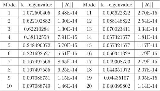
Table 3.1 Verification of the flux harmonics obtained by QZ decomposition for a PWR assembly . . . 27 Table 3.2 Verification of the flux harmonics obtained by QZ decomposition for a

CANDU-6 supercell . . . 33 Table 3.3 Verification of the flux harmonics obtained by deflation for a PWR

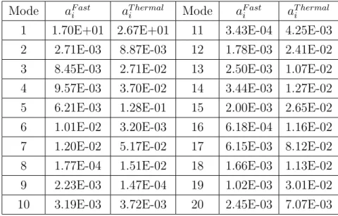
assembly . . . 35 Table 4.1 Fuel composition of a PWR assembly at mid-burnup . . . 45 Table 4.2 Absolute value of the amplitudes of the 20 most dominant modes . . 50

(14)

LISTE OF FIGURES

Figure 3.1 17 × 17 PWR fuel assembly . . . 26

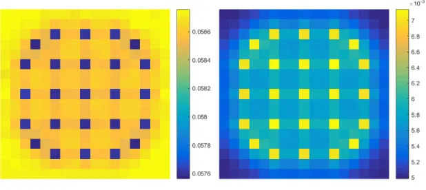
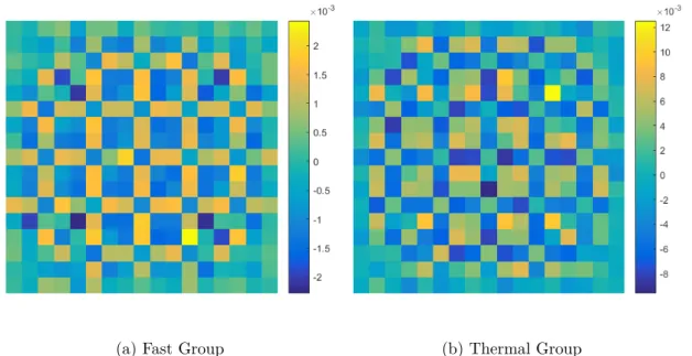
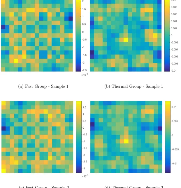
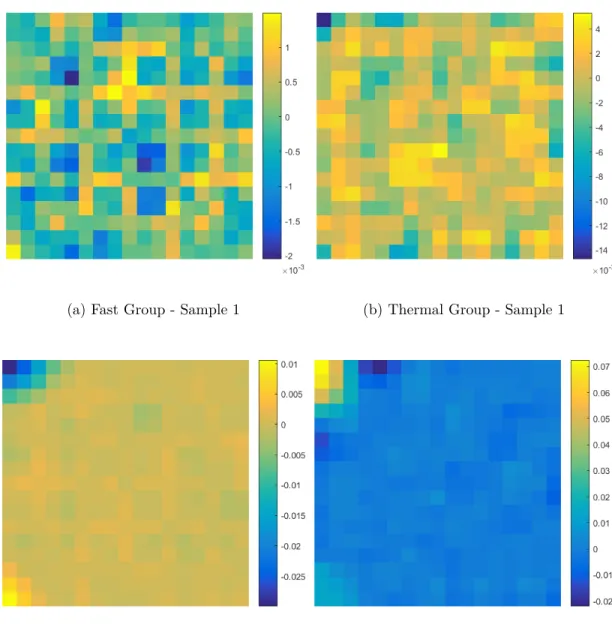
Figure 3.2 QZ modes 1-8 in the fast group for a PWR fuel assembly . . . 28

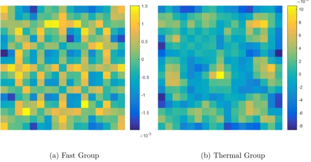
Figure 3.3 QZ modes 1-8 in the thermal group for a PWR fuel assembly . . . 29

Figure 3.4 CANDU-6 supercell of 4 × 4 unit cells . . . 30

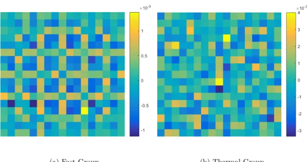
Figure 3.5 QZ modes 1-6 in the fast group for a CANDU-6 supercell . . . 31

Figure 3.6 QZ modes 1-6 in the thermal group for a CANDU-6 supercell . . . . 32

Figure 3.7 PWR 3 × 3 supercell . . . 37

Figure 3.8 Diffusion solution in the thermal and fast groups for a partial PWR core 38 Figure 3.9 Relative error between diffusion solution and MC reference in the ther-mal and fast groups for a partial PWR core . . . 39

Figure 3.10 Relative error between reconstructed homogeneous solution and MC reference in the thermal and fast groups for a partial PWR core . . . 39

Figure 3.11 Constructed neutron flux map on a fine mesh in the thermal and fast groups for a partial PWR core . . . 40

Figure 3.12 Relative error between constructed detailed flux map and MC reference in the thermal and fast groups for a partial PWR core . . . 41

Figure 3.13 Relative error between constructed pin-wise fission rate and MC refer-ence in the thermal and fast groups for a partial PWR core . . . 42

Figure 4.1 MC solution for the neutron flux in a PWR assembly . . . 46

Figure 4.2 Relative differences between MC solution and fundamental mode solu-tion of the flux in a PWR assembly . . . 47

Figure 4.3 Relative difference between MC solution and neutron flux reconstructed using 264 dominant modes . . . 48

Figure 4.7 Relative difference between MC solution and neutron flux reconstructed using 20 dominant modes assuming uniform mapping error . . . 53

Figure 4.8 Relative difference between MC solution and neutron flux reconstructed using 89 dominant modes assuming uniform mapping error . . . 53

(15)

Figure 4.9 Relative difference between MC solution and neutron flux reconstructed using 264 dominant modes assuming uniform mapping error . . . 54 Figure 4.10 Relative difference between MC solution and neutron flux reconstructed

using 20 dominant modes assuming absorption related mapping error 55 Figure 4.11 Relative difference between MC solution and neutron flux reconstructed

using 20 dominant modes and 100 random tallies . . . 58 Figure 4.14 Histogram of the maximum absolute relative error on the reconstructed

MC flux using 20 dominant modes and 100 random tallies . . . 59 Figure 4.15 Relative difference between MC solution and neutron flux reconstructed

using 50 dominant modes and 100 random tallies . . . 60 Figure 4.16 Histogram of the maximum absolute relative error on the reconstructed

MC flux using 50 dominant modes and 100 random tallies . . . 61 Figure 4.17 Relative difference between MC solution and neutron flux reconstructed

using 20 dominant modes and 100 random tallies with IRWLS . . . . 64 Figure 4.18 Histogram of the maximum absolute relative error on the reconstructed

MC flux using 20 dominant modes and 100 random tallies with IRWLS 65 Figure 4.19 Relative difference between MC solution and neutron flux reconstructed

using 50 dominant modes and 100 random tallies with IRWLS . . . . 66 Figure 4.20 Histogram of the maximum absolute relative error on the reconstructed

MC flux using 50 dominant modes and 100 random tallies with IRWLS 67 Figure 4.21 Weights of different cells in the calculation of modal amplitudes as

determined by IRWLS using 20 dominant modes . . . 68 Figure 4.22 Weights of different cells in the calculation of modal amplitudes as

determined by IRWLS using 50 dominant modes . . . 68 Figure 4.23 Weights of different cells in the calculation of modal amplitudes as

determined by IRWLS using 20 dominant modes and a diffusion solution 69 Figure 4.24 Weights of different cells in the calculation of modal amplitudes as

determined by IRWLS using 50 dominant modes and a diffusion solution 70 Figure 4.25 Relative error on the reconstructed neutron flux from tallies in 100 cells

of largest weights and 20 modes . . . 71 Figure 4.26 Relative error on the reconstructed neutron flux from tallies in 100 cells

(16)

Figure 5.1 Flow chart of the hybrid method . . . 74 Figure 5.2 Reference fine mesh MC solution for the neutron flux in a PWR assembly 75 Figure 5.3 Calculation of the macroscopic cross sections in the MC solver . . . . 76 Figure 5.4 Relative errors between reference fine mesh MC solution and the flux

reconstructed from 20 dominant modes . . . 77 Figure 5.5 Relative errors between reference fine mesh MC solution and the flux

reconstructed from 200 dominant modes . . . 79 Figure 5.8 Reference fine mesh MC solution for the fission rate in a PWR assembly 80 Figure 5.9 Relative errors between reference MC solution and the fission rate

dis-tribution reconstructed from 50 dominant modes . . . 80 Figure 5.10 Relative errors between reference fine mesh MC solution and the flux

reconstructed from 20 dominant modes plus estimated error . . . 82 Figure 5.11 Relative errors between reference fine mesh MC solution and the flux

reconstructed from 200 dominant modes plus estimated error . . . 83 Figure 5.14 Reference fine mesh MC solution for the flux distribution a PWR 3 × 3

supercell . . . 84 Figure 5.15 Reference fine mesh MC solution for the fission rate in a PWR 3 × 3

supercell . . . 85 Figure 5.16 Relative errors between reference fine mesh MC solution for a PWR

3 × 3 supercell and reconstructed flux using modal expansion - case 1 86 Figure 5.17 Relative errors between reference fine mesh MC solution for a PWR

3 × 3 supercell and reconstructed fission rate using modal expansion -case 1 . . . 86 Figure 5.18 Relative errorss between reference fine mesh MC solution for a PWR

3 × 3 supercell and reconstructed flux using modal expansion - case 2 87 Figure 5.19 Relative errors between reference fine mesh MC solution for a PWR

3 × 3 supercell and reconstructed fission rate using modal expansion -case 2 . . . 88

(17)

Figure 5.20 Reference fine mesh MC solution for the flux distribution a PWR 3 × 3 supercell in axial plane 1 . . . 89 Figure 5.21 Reference fine mesh MC solution for the flux distribution a PWR 3 × 3

supercell in axial plane 2 . . . 89 Figure 5.22 Reference fine mesh MC solution for the flux distribution a PWR 3 × 3

supercell in axial plane 5 . . . 91 Figure 5.26 Relative errors between MC reference solution and reconstructed flux

map in axial plane 1 . . . 92 Figure 5.27 Relative errors between MC reference solution and reconstructed flux

map in axial plane 5 . . . 94 Figure 5.31 Relative errors between MC reference solution and reconstructed fission

rate map in axial plane 1 . . . 95 Figure 5.32 Relative errors between MC reference solution and reconstructed fission

rate map in axial plane 5 . . . 95 Figure 5.33 Relative errors between reference fine mesh MC solution and the flux

reconstructed at 0MWd/Kg burnup - case 1 . . . 98 Figure 5.34 Relative errors between reference fine mesh MC solution and the flux

(18)

Figure 5.38 Relative errors between reference fine mesh MC solution and the flux reconstructed at 5MWd/Kg burnup - case 1 . . . 100 Figure 5.39 Relative errors between reference fine mesh MC solution and the flux

(19)

CHAPTER 1 INTRODUCTION

The design, analysis and operation of nuclear fission reactors depend on understanding the rates of different neutron reactions within the reactor core. For this purpose, the neutron flux distribution over the core needs to be estimated with good confidence. Since the discovery of nuclear fission and the introduction of nuclear reactors, different deterministic and stochastic approaches have been developed for modelling reactor cores and studying the neutron flux distribution.

Deterministic methods are mathematical approaches developed to find an approximate solu-tion for the Boltzmann neutron transport equasolu-tion which states the law of conservasolu-tion of neutrons. Given the complexity of reactor configurations, it is almost impossible to find an analytical solution of the transport equation and numerical methods based on direct discreti-sation of the independent variables demand extreme computing resources. Hence, several simplifications in the elements defining the problem (geometry, neutron energy, etc.) are ap-plied. Current practice in deterministic methods is based on a two steps process comprising a lattice calculation for a single unit cell followed by a diffusion calculation for a simplified reactor geometry. In the lattice calculation, the reactor is represented by a single unit cell that defines the characteristics of the reactor and extends in an infinite lattice. The transport equation is numerically solved on a detailed spatial mesh and a relatively large number of neutron energy groups. The lattice solution is then condensed, both in space and energy, to compose a reactor database that can be utilised in the next step. The second step is a low order approximation, such as diffusion, where the reactor is represented by a finite domain of homogenised unit cells and an approximate integral solution is calculated. The lattice solution is then imposed on the low order one using form functions and form factors and fuel optimisation and reactor safety analysis are performed. Due to the number of simplifications involved in deterministic methods, the accuracy of the solution is jeopardised and large safety margins are applied in design and optimisation of reactor cores. [1]

On the other hand, stochastic methods are statistical approaches used to simulate the physical behaviour of neutrons within the reactor core. Unlike deterministic methods, stochastic ap-proaches such as Monte Carlo require few simplifications in defining the problem; this method can handle very complex geometries and can treat neutron properties in the continuous do-main. Typically, a Monte Carlo simulation follows the history of a number of neutrons along their path from the point of birth to the point of consumption or removal. Along this path, different reactions or interactions are sampled based on provided probability distributions.

(20)

A statistical estimate of the neutron population is then obtained from the average behaviour of the neutron histories. Due to the stochastic nature of the simulation and the limited number of simplifications applied, the Monte Carlo method presents a superior approach to deterministic methods in terms of accuracy and confidence in the solution. However, despite the advancement of computing platforms, the computational burden encountered in full core Monte Carlo simulations renders it impractical for production calculations and the method has been limited in reactor physics to benchmarking. [2]

1.1 Problem Formulation

With the introduction of new nuclear fuels, advanced fuel cycles and novel reactor designs, there is a growing need for advanced and accurate methods in reactor physics. Current trend within the research community shows a renewed interest in the Monte Carlo method and efforts focus on improving its performance through reducing the computational costs. Recently, it has been recognised that some improvement in the performance of Monte Carlo can be achieved through coupling the stochastic method with deterministic approaches. In particular, such hybrid approaches are utilised for accelerating the inactive portion of the Monte Carlo simulation which is used to converge the fission source of which neutrons are sampled [3]. Nevertheless, the inactive portion of the Monte Carlo simulation comprises less than 2% of the total run; any acceleration of the inactive cycle remains insignificant.

In this work, a new hybrid method based on coupling a stochastic solver to a deterministic flux mapping algorithm for reducing the computing time for full core calculations is developed.

1.2 Research Definition and Aims

Unlike current hybrid methods, the described approach does not aim to accelerate the stochas-tic solver. Rather, the approach combines a continuous energy continuous space domain stochastic solver with a deterministic multi-energy groups flux mapping algorithm to study full core neutronics within reasonable computational time and expense, while maintaining good accuracy compared to the Monte Carlo method.

In the proposed approach, the Monte Carlo solver is used to estimate the neutron flux in a limited number of regions over the reactor core and to produce a set of few energy groups neutron cross sections. A deterministic solver uses the generated data from the Monte Carlo run to solve the transport equation or one of its approximations in a lattice calculation and obtain the high order modes over a single unit cell. Then, flux mapping using the high order dominant modes and the Monte Carlo tallies are utilised to construct the neutron flux

(21)

distribution over the complete spatial domain. By reducing the number of regions tallied by the stochastic solver, reduction in both the computing time and memory demand can be achieved.

Development of the hybrid method is undertaken with the aim of completing a full core neu-tronics simulation with a running time that should be at least 50% faster than conventional Monte Carlo. The target accuracy of the solution is 5% or better on the fission rate when compared to a reference Monte Carlo solution.

In order to achieve the aims stated above, the following methodology is applied: • Investigate the feasibility of the proposed hybrid method.

• Evaluate different mathematical approaches for performing neutron flux mapping. • Implement a dominant modes solver in the lattice code DRAGONv5.

• Implement the hybrid method and perform sample reactor physics studies.

• Identify strengths and weaknesses of the hybrid method and recommend improvements.

1.3 Thesis Structure

This thesis proceeds by a literature review of the Monte Carlo (MC) method, challenges for full core MC and a brief description of few MC codes. Chapter 3 deals with the transport equation and its solutions. A brief literature review on the transport equation is provided. Mathematical methods for obtaining the high order modes are described with some sample calculations. The chapter concludes with an introduction to the concept of flux mapping and its application for finding a solution for the transport equation. In chapter 4, the feasibility of the hybrid method is investigated through reconstructing a MC solution in a single PWR fuel assembly using the dominant modes and flux mapping. Practical implementation and application of the method to 2D and 3D problems are presented in chapter 5. The per-formance of the method is compared against the conventional Monte Carlo method. The work concludes by a summary of the results, identification of the deficiencies of the proposed hybrid method and suggestions for future developments.

(22)

CHAPTER 2 LITERATURE REVIEW

In this chapter, a literature review of the Monte Carlo method is presented. A brief descrip-tion of the theory of MC is included. Then, challenges for full core MC neutronic simuladescrip-tions are described with different approaches for tackling these challenges. Recent hybrid methods used for accelerating the inactive portion of the simulation are reviewed. Finally, a presen-tation of some of the MC codes developed or under development for full core reactor physics is included.

2.1 The Monte Carlo Method

Unlike deterministic methods, the Monte Carlo approach does not solve an integral or dif-ferential equation. Rather, the method attempts to follow the behaviour of neutrons as they transport across the reactor core. In this sense, the method can be viewed as a virtual reactor on a computer.

From the point of their introduction to the point of removal, neutrons can undergo different types of interactions with nuclei in the medium. Such interactions are governed by probability distributions related to the neutron cross sections and properties of the medium, energy of neutrons and their direction of travel. The Monte Carlo method tracks a large number of neutrons, one by one, and determines the most probable interactions they would undergo through their history. The neutron flux distribution is then estimated by observing the average behaviour of tracked neutrons.

Between points of interactions, neutrons travel in straight paths. For a neutron of a given energy E, the probability of it surviving an interaction in the medium after travelling a distance l and then colliding in dl is given by [4]:

P (l)dl = Σt(E)e−Σt(E)ldl (2.1)

where P (l) is the collision probability in dl, Σt is the total macroscopic neutron cross section. The history of a neutron proceeds by sampling from a set of sources distributed across the core. At an initial point of known coordinates, pseudo-random numbers are generated and statistical tests are performed to determine the initial neutron energy and its direction of travel. Another pseudo-random number is generated and compared to the cumulative probability distribution function corresponding to the probability distribution function of equation eq. (2.1) to sample a neutron path length. If the neutron does not cross an interface

(23)

along its path, it is moved to the point of interaction, otherwise the track length is reduced to the distance to the interface. At the point of interaction or interface, a pseudo-random number is generated and statistical tests are performed to determine the type of interaction. If the interaction is a scattering reaction, the energy and direction of travel are updated. If absorption is sampled, a statistical test is performed to determine the type of absorption. When fission or neutron emitting reaction occurs, neutron sources to be used in the next cycle are updated. Tracking of a neutron continues until it leaks outside the reactor domain or until removed by absorption. The process is repeated for a large number of neutron histories and simulation cycles. [2, 5]

The neutron flux distribution is estimated using one of two estimators. The track length estimator calculates the flux distribution in a given volume from the total length travelled by neutrons within the volume:

φ(~Ω, E) = 1 nN V N X j=1 n X i=1 wj_i lj_i(~Ω, E) (2.2)

where φ(~Ω, E) is the flux within a tally cell of volume V , n is the number of neutron histories per cycle, N is the number of cycles, w_ij is the statistical weight of the ith _{particle in the j}th cycle and l_ij(~Ω, E) is the track length of the ith_{particle of the j}th_{cycle along direction Ω with} energy E within the tally cell. Alternatively, the collision estimator calculates the neutron flux distribution by recording the number of collisions scored within a given tally cell:

φ(E) = 1 nN V N X j=1 n X i=1 wj_i Σt(E) (2.3)

Accuracy of the solution is influenced by different factors such as the effort used in defining the problem, accuracy of nuclear data and the number of neutron histories tracked. The confidence in the estimate is typically determined in terms of the standard deviation σ which is calculated according to [2]: σ2 = 1 N − 1 N X i [φi− φ]2 (2.4)

where N is the number of samples, φi is the estimate of the flux by the i − th sample and φ is the mean flux.

(24)

2.2 Challenges for Full Core Monte Carlo

Challenges for full core MC simulations can be described in two general categories, those inherent to the MC method and those arising from the physical nature of the problem. The second category becomes particularly important when multiphysics feedback is studied. In-herent challenges include the long computational time for acceptable results, large demand for computing memory, slow convergence of the source distribution as well as variance esti-mation. The origins of these as well as methods available to address them are reviewed in the subsequent sections.

2.2.1 Accounting for Multiphysics Feedback

Coupling MC simulations to multiphysics feedback such as fuel burnup and thermal-hydraulics poses a challenge for the development of MC as a mainstream reactor analysis tool as opposed to its traditional benchmarking role. The origin of this challenge lays in three issues: the inherent fluctuations of the MC solution, the discontinuous nature of the MC solution and the calculation of temperature dependant neutron cross section data [3]. In addition, taking into account the dynamic evolution of the reactor due to isotopic depletion or accumula-tion has its impact. The MC soluaccumula-tion comprises a number of stochastic simulaaccumula-tions of the physical behaviour of neutrons. The random nature of the simulation introduces significant fluctuations over different cycles. These fluctuations could introduce convergence issues for mutliphysics solvers which represents an outstanding issue that need to be addressed in de-veloping new MC codes [3]. Furthermore, the MC solution is typically given in the form of a discontinuous tally histogram while multiphysics solvers rely on continuous physical models and data. Hence, there is a requirement for developing methods for calculating continuous tally data. Two methods are currently available to produce continuous MC tallies. These are the Functional Expansion Technique [6] and the Kernel Density Estimator [7]. Finally, an efficient approach for calculating the temperature dependent neutron cross section data is required to account for the different temperatures observed across the reactor. Temperature dependent cross section data can be calculated a priory on a fine or a coarse temperature mesh and an interpolation can be done to retrieve the cross section data at the required temperature [3]. A better approach is the on-the-fly Doppler broadening where only data at a reference temperature are stored and these are broadened to produce the data at the required temperatures when needed [8]. When fuel burnup is considered, it is necessary to obtain detailed flux distribution within fuel pins which means tallying on a very fine mesh. Furthermore, accurate flux distribution and reaction rates are required for burnup studies which necessitates increasing the number of histories to improve the simulation statistics.

(25)

The consequences are longer run times as well as an increase in the memory demand. Fur-ther illustrations on the relation between the computation costs and the number of histories or tallies can be found in subsequent sections.

2.2.2 Computational Time

MC estimate of the neutron flux is a statistical average of a number of tracked neutrons across the reactor geometry. The accuracy of the estimate is improved by increasing the number of neutron histories simulated according to the law of large numbers. The total time required by a MC run to obtain the flux distribution is proportional to the number of tracked neutrons and the time required per neutron history [3]. Smith [9] considered a LWR (Light Water Reactor) core with 70000 pins and estimated that 100 billion neutron histories are required to obtain a standard deviation of 1% on the neutron flux. This implies that the computational time would be prohibitively high on simple computer architectures such as PCs. Smith has estimated the time required to perform a full core calculation with fuel burnup to be about 5000 hours on a 2GHz PC [10]. Since the number of neutron histories required is also dictated by the size and configuration of the reactor, efficient reduction of the total time required by MC simulations can be only achieved by reducing the time required per neutron history. This depends on several factors such as the number of spatial points (meshes) where the flux is to be estimated, the number of tallies and availability of computer memory [3].

2.2.3 Memory Demand

The memory requirement of a MC simulation of a reactor core is imposed by three factors [3]: the simulated physical quantities (tallies), the cross section data and the geometry of the reactor. Typically, the neutron flux distribution on a fine mesh of the phase space is the main tally of a MC simulation. In addition, when the dynamic behaviour of the reactor is considered, additional tallies to account for fuel burnup and depletion/accumulation of isotopes are required. The total memory requirement for tallying is proportional to the number of regions tallied, the number of physical quantities recorded per region and the required accuracy of the estimates. Smith [9] evaluated the memory demand for a typical LWR core with 70000 pins. For the required 1% statistics on the neutron flux, he estimated that 10 radial and 100 axial meshes per fuel pin will be required; thus, a total of 70 millions tally regions. He also considered that 300 isotopes are to be tracked (which drives the number of tallies up) and allowed additional memory requirements for variance estimation. Assuming 8 bytes per tally, a rough estimate of the memory demand for a MC simulation of an LWR is

(26)

1 TB. The memory requirements are much larger if other phenomena such as the rim effect [11] and multiphysics feedback or advanced fuel designs are considered [3].

The geometry of the reactor also has an impact on the memory demand. This depends on the size of the reactor and the degree of details required from the simulation. On the other hand, memory demand by cross sections and isotopic data depends on the number of isotopes tracked [3]. When dynamic studies are considered, a large number of isotopes are tracked and the nuclear data for these must be stored. Given the wide temperature range within the reactor core, cross sections data are required at different temperatures to account for the Doppler broadening effect. Thus, significant memory is required for storing the cross sections. However, on flight calculation [8] of the temperature dependent cross sections from the stored 0 K data can be utilised to reduce the memory demand by cross sections.

2.2.4 Convergence of the Fission Source

MC simulations rely on sampling neutrons and their spatial position, energy and direction of travel from a sample that effectively represents the general population of neutrons. In criticality MC studies, neutrons are sampled in consecutive cycles from the set of neutrons born from fission reactions in previous cycles. Thus, MC simulations are performed in two stages, a number of inactive cycles where no tallies are recorded followed by active cycles to estimate the required tallies. The first stage is used to converge the fission source spatial distribution that is to be used in neutron sampling. Conventional MC simulations suffer from very slow convergence of the fission source [3]. Hence, some acceleration schemes are required to increase the efficiency of MC runs. Acceleration methods include the fission matrix approach, importance sampling and hybrid deterministic-stochastic methods.

Fission Matrix Approach

The fission matrix approach [12] was initially applied to accelerate the convergence of fission source spatial distribution in criticality safety calculations and was later extended to full core studies. The method builds on the fact that the fission source distribution is an eigenvector that satisfies the following relation:

HS = 1

kS (2.5)

where S is the energy integrated fission source spatial distribution vector, k is the multipli-cation factor and H is the fission matrix. The elements of the fission matrix Hij represent the number of fission neutrons created in a region i of the reactor domain due to the fission caused by a neutron born in region j of the domain. The elements of the fission matrix can

(27)

be determined by tallying the neutron transfer and fission rates during the MC run. Once the fission matrix is determined, the smallest eigenvalue (i.e. the largest k) and the corre-sponding eigenvector are determined by solving eq. (2.5). Hence, the accuracy of the fission source distribution relies on accurate estimation of the fission matrix. However, only a rough estimate of the matrix H is required to accelerate the convergence of the source distribution. The process is repeated in subsequent cycles until a converged fission source is obtained to start the active cycles. The main advantage of this method is the significant reduction in the number of inactive cycles as compared to the conventional iterative solution applied in conventional MC. [12]

Importance Sampling

Importance sampling is an approach borrowed from variance reduction techniques to accel-erate the convergence of the fission source term [3]. The convergence of the fission source distribution is particularly slow when the simulated core is relatively large, characterised by a high dominance ratio [3]. This occurs when the distribution of fission neutrons converges in some regions while a reliable distribution is not obtained yet in many different regions. Thus, a large number of inactive cycles is required to ensure a reliable distribution is obtained everywhere in the reactor core. In the importance sampling approach, neutron sampling is biased such that regions that would require longer time to converge are sampled more fre-quently and a converged source is obtained in fewer cycles. One approach to importance sampling in criticality problems is the Forward Weighted Consistent Adjoint Importance Sampling (FW-CADIS) developed at ORNL [13]. In this approach, a deterministic adjoint calculation is performed to obtain the biasing weights for the MC run. This method is based on the fact that the physical significance of the adjoint flux is to quantify the contribution or importance of a particle to the overall flux or particular reaction rate. A deterministic calculation, typically SN, is first performed to obtain an approximate solution of the flux Ψ(~r, E, ~Ω). This is then used to calculate an adjoint source [13]:

q+(~r, E) = νΣf(~r, E)

R R

Ψ(~r, E, ~Ω)νΣf(~r, E)dEd2Ω

(2.6)

where q+ _{is the adjoint source and νΣ}

f(~r, E) is the neutron production cross section with ν being the average number of neutrons produced per fission reaction. Next, an adjoint calculation is performed to calculate the adjoint flux distribution Ψ+_(~_{r, E, ~}_{Ω). Finally, the}

(28)

space-energy-angle dependent neutron weights are evaluated:

w(~r, E, ~Ω) =

R R

Ψ(~r, E, ~Ω)νΣf(~r, E)dEd2Ω

Ψ+_(~_{r, E, ~}_Ω) (2.7)

It has been reported that the FW-CADIS method was successfully employed to speed up the convergence of the fission source in a full core MC calculation up to seven times [13].

Hybrid Methods

Hybrid deterministic-stochastic methods are developed based on the fact that the calculation of the fission source distribution is the same in both approaches. Several hybrid methods were developed; of which the most popular is the Coarse Mesh Finite Difference (CMFD) [14]. In the CMFD method, the fission source distribution is obtained by solving a multigroup neutron conservation equation over a coarse discretisation of the reactor domain. The neu-tron conservation equation is obtained by integrating the steady state Boltzmann transport equation over the solid angle:

∇Jg(~r) + Σtg(~r)φg(~r) − G X g0₌₁ Σg0_→gφ0 g(~r) = χg k G X g0₌₁ νΣf g0(~r)φ_g0(~r) (2.8)

where Jg(~r) is the neutron current in energy group g, φg is the group neutron flux, and k is the eigenvalue (multiplication factor). Note that only one fissile isotope is considered for the simplicity of notation. If the spatial domain is discretised, a similar equation can be written to state the conservation of neutrons within the mesh cells. For a cell of index m:

Ns m X s=1 Am s Vm Js_g+ Σm_tgφm_g − G X g0₌₁ Σm_g0_→gφ 0m g = χg k G X g0₌₁ νΣm_{f g}0φ m g0 (2.9) where Ns

m is the number of surfaces bounding the mesh cell, J s

is the average net neutron current passing across surface s of cross section Am

s , φ is the average neutron flux inside the mesh cell and the macroscopic cross sections are taken as the average inside the cell. To solve the above equation, a relation between the neutron current passing the surfaces of the mesh cell and the neutron flux inside it is required. A convenient approach is obtained by defining a current to flux conversion factor ( ˜D) using Fick’s law (J = −D∇φ). Finite discretisation results in [15]:

Jg s

= − ˜Ds_g(φm−1_g − φm

(29)

where ˜Ds g =

2Dm−1g Dmg

hm−1_Dm−1 g +hmDgm

results from the finite discretisation of the diffusion equation and is a function of the diffusion coefficients and the mesh size hm, φm−1 is the average flux in the mesh cell to the left of the surface s and φm is the average flux in the right side cell. The validity of the above relation is challenged unless the mesh size is sufficiently small and the medium is highly scattering with weak neutron absorption. For a coarse mesh, a modified relation replaces the above equation by:

Jgs = − ˜D_gs(φm−1_g − φm_g ) + ˆD_gs(φm−1_g + φm_g ) (2.11) where ˆD_gs is a correction factor obtained from a reference high-order or fine mesh calculation of the current and the flux in the neighbouring cells:

ˆ D_gs = J ∗s g + ˜D∗sg (φ∗m−1g − φ∗mg ) (φ∗m−1 g + φ∗mg ) (2.12)

The asterisk denotes a value obtained from a reference calculation. Once the relation between the current and the flux is known, a system of coupled equations is obtained that can be solved to calculate the flux in each mesh. The resulting flux is employed for calculating the fission source density to be used in the criticality calculation. The coupled CMFD-MC utilised to estimate the fission source density is an iterative method where MC is used to obtain the reference flux (φ∗_{), the reference current (J}∗_{) and cross sections for calculating}

ˆ Ds

g. This approach proceeds by running the MC solution for a number of inactive cycles in order to obtain a semi-converged fission source distribution. The semi-converged solution is employed to calculate the coefficients ˜Ds

g, ˆDsg, Σtg, Σg0_→gand νΣ_{f g} of the coarse mesh system

given by eq. (2.9) and eq. (2.11). Once the deterministic system is solved over all the mesh cells, the fission source distribution is calculated and is used in the next cycle of the MC calculation: Sm = χg k G X g0₌₁ νΣm_{f g}0φ m g0

where Sm_{is the energy group fission neutron source within the cell m. The process is repeated} until a converged fission source distribution is obtained [15]. The CMFD-MC method was successfully employed to reduce the number of the inactive cycles by a factor of 26 in an exemplar 3D problem as reported in [15].

Other hybrid methods were developed such as the Function Monte Carlo Method (FMC) [16]. Currently, the FMC method is limited to 1D geometries and thus is not of great interest in the context of this document. Finally, although hybrid methods described in literature achieve some acceleration, any improvement brought by these methods are marginal. All current

(30)

hybrid methods concentrate on the acceleration of the inactive cycles of the MC simulation; these constitute less than 2% of the complete simulation.

2.2.5 Variance Estimation

The error estimator based on the central limit theorem, eq. (2.4) would be correct if the simulation cycles were independent, one of each other. However, since neutrons in successive cycles are sampled from those estimated in the previous one, a bias is introduced into the final result due to an intercycle correlation [17]. This introduces a discrepancy between the estimated standard deviation obtained by the CLT (denoted “apparent variance”) and the actual value (denoted “true variance”) [18]. It has been reported that the ratio between the true to apparent variances is between 2-5 [19, 14]. Design and safety analysis of the reactor core require high confidence in the estimated flux which means that the discrepancy between the true and apparent variance cannot be ignored. Hence, new approaches are required to reduce the underestimation in the standard deviation of a MC simulation.

Four approaches are proposed for reducing the discrepancy between the apparent and the true variance. The Gelbard’s batch approach [20] estimates the tallies from a batch of cycles rather than separate cycles. The standard deviation is calculated for the batch averages. The advantage of this approach is reducing the inter-cycle correlation by using the averages of a number of cycles rather than single cycles. The Ueki’s [17] approach attempts to estimate the inter-cycle correlation by using the autocovariance of the successive cycles which can be calculated from the cycle averages. By estimating the bias, a correction can be made to the apparent variance and a better estimation of the uncertainty is obtained. Another approach based on the stochastic error propagation model [21] is utilised to estimate the inter-cycle correlation and provide an estimate of the true variance. Finally, the history-based batch method [22] attempts to better estimate the variance by eliminating the inter-generational dependence of the fission source distribution. This is achieved by treating a MC simulation of N cycles and M histories as a number of independent runs NB each with N cycles and

M

NB histories per run. That is, the number of neutron histories simulated are split over the

number of repeated runs, called history batches, which are independent of each other.

2.3 Global Acceleration Techniques

Global acceleration of MC full core simulations can be achieved by reducing the time required per history as well as by reducing the total number of histories required for given statistics. Apart from using faster computers, a reduction in the time required per neutron history became feasible with modified tracking techniques. Reduction in the number of histories

(31)

while maintaining the same confidence in the results can be achieved by employing variance reduction techniques.

In analogue MC simulations, all neutrons are characterised by the same statistical weight. Neutron histories that are unlikely to contribute to the final tally are tracked from origin point until capture or leakage; such an approach is wasteful. Variance reduction techniques act as a filter to distinguish between neutrons contributing to the result and those having low or no contribution. Several approaches are available including splitting and roulette, implicit capture and interaction forcing. The splitting roulette approach is widely used in several MC codes. The basic idea is to split particles with expected high contribution to the result into a number of particles with same characteristics of the original particle. The split particles are tracked independently and share the same statistical weight. On the other hand, particles with unlikely contribution are subject to a statistical test. A random number is sampled and if this number falls below a predetermined threshold, the history is terminated, otherwise, tracking continues and the weight of the particle is increased. In the implicit capture method, no absorption reactions are allowed. When an absorption reaction is sampled from the cross section data, the neutron history is not terminated. Instead, the weight of the neutron is reduced by the probability of absorption. This approach is combined with Russian Roulette to terminate the histories of those neutrons whose weights become less than a user defined threshold. The implicit capture approach ensures that particles with low weight will have some contribution to the tallies. Finally, interaction forcing approach is used to ensure regions of high importance but small dimensions in the order of a mean free path are sampled more frequently. Sampling of the next collision site near such regions is modified to force some interactions within the region while adjusting the weight of the history. [23]

At the heart of the MC simulation is tracking of neutrons while they travel through the geometry from the point of origin to removal is followed. Tracking is a strong function of the geometry and becomes more lengthy as the complexity of the geometry increases. In the conventional form, the straight line distance travelled by a single neutron before undergoing an interaction is decided by sampling a mean free path using the total macroscopic cross section. If the neutron is to cross an interface between different material regions before making a collision, the travel distance need to be adjusted and sampling a new mean free path is required. The distance between the point of origin to the nearest interface is determined recursively from the sampled point of interaction. The process becomes very lengthy when the geometry comprises different heterogeneities. [23]

An alternative approach which reduces the dependence on the geometry is the delta tracking method; full details are given in [24]. In this approach, the concept of a virtual collision during which the neutron neither changes its energy or direction of travel is introduced. The

(32)

purpose of this virtual collision is to modify the total cross sections in all regions such that the whole system is characterised by a uniform interaction probability. Mathematically, the virtual cross section is given by:

Σ0(~r, E) = Σm(E) − Σt(~r, E) (2.13) where Σ0(~r, E) is the local virtual collision macroscopic cross section, Σm(E) is the maximum total cross section (majorant) among all materials in the system and Σt(~r, E) is the local total cross section. Delta tracking is initiated by sampling a mean free path using the majorant cross section. After moving the neutron to the new location, the type of collision is determined whether virtual or physical. The probability of a virtual collision (Pv) is given by:

Pv = 1 −

Σ0(~r, E)

Σm(E)

(2.14)

If a physical interaction is sampled, the neutron characteristics are modified accordingly, otherwise a new mean free path is selected. Since the interaction probability is uniform over the system, tracking becomes independent of the geometry. This method is not error free. When the geometry contains localised strong neutron absorbers, the virtual collision cross section becomes dominated by the absorption cross section of the strong absorbers. Since these absorbers are present in small regions, the probability of neutrons interacting in such regions is relatively small. Hence, the rate of virtual collisions will be large and time is wasted by resampling. An extended version to overcome this limitation was developed by Leppänen [24]. In the modified version, a second majorant cross section is defined as the maximum total cross section of all materials excluding localised absorbers. If the difference between the two majorants is significantly large at a given energy, the mean free path is sampled using the second majorant. The distance to the nearest absorber is determined; if the neutron crosses the surface of an absorber along the sampled travel line, the mean free path is adjusted and a new mean free path is sampled using the first majorant [24]. This process is employed in the Serpent code and is the major contributor to its accelerated performance.

2.4 Full-Core MC Codes

In this section, a brief description of some of the MC codes being developed for full-core reactor physics analysis is presented. For brevity, emphasis is given on the distinctive features of these codes. The review includes the MC21, MCCARD, Serpent and OpenMC.

(33)

2.4.1 MC21

The MC21 code is being developed by Knoll’s Atomic Power Laboratories and Bettis Atomic Power Laboratories as a part of a wider project to develop a MC based nuclear reactor design and analysis tool [25].

The code utilises continuous energy cross section data from common nuclear data libraries. The nuclear data are processed by a system of codes called Nuclear Data Extractor (NDEX) that read the data from ENDF, EPDL or ACE files stored in a Nuclear Data Repository (NDR) and produces data libraries for the specific MC21 run. The NDR contains data files for different elements in the form of several versions corresponding to different data libraries. Data processed by NJOY are stored in the NDR for use in MC21 simulations. When a job is executed, NDEX checks for the availability of required data in the NDR and copies these to a library file. Data not readily available in the NDR are processed by NJOY and stored in the NDR for future use. This reduces the computational expense for nuclear data processing as data at given conditions are processed only once and stored in the repository. [26]

The MC21 [25] code allows for modelling complex 3D geometries via a “flexible 3D combi-national geometry coupled with dedicated geometry kernels for common shapes” [26]. The geometry definition is based on four elements: quadratic surfaces that define the bound-aries/interfaces, components that define volumes bounded by intersection or union of sur-faces, grids that allow the definition of geometrical details in a component and overlays that allows the definition of geometrical details inside a grid cell. In addition, MC21 allows the definition of movable geometries, a feature that is particularly useful for the representation of control rods. [25, 26]

Neutron flux tallying in MC21 is based on the standard track length estimator. Typically, a tally X is calculated by the integral:

X = Z dr Z d2Ω Z dR f (~r, ~Ω, E)φ(~r, ~Ω, E) (2.15) where the user specifies the limits of the integration to define a mesh cell in the phase space as well as the function f (~r, ~Ω, E) to determine the physical property to be tallied. For example, a reaction rate can be tallied by setting f to be the macroscopic cross section of the reaction of interest. The tallies of MC21 are written in the form of a census rather than integral tallies. Census tallies record the history of individual particles simulated including their de-tailed phase space coordinates and their statistical weight. The advantage of this approach is to enable the use of these histories in future simulations. Particle sources can be specified from predefined distributions or can be sampled from stored censuses obtained from previous results. The latter is particularly useful for accelerating the convergence of the fission source

(34)

distribution in criticality simulations. In addition, the efficiency of the tallying process is ensured through storing the tallies in hashed arrays which reduces the computational time for the tallying process.[25, 26]

The code is developed to perform full-core reactor calculations with the capability of coupling to multiphysics effects such as thermal-hydraulics, xenon feedback, heating and control de-vice motion. An internal thermal feedback module calculates the thermal distribution across the geometry based on user defined heat transfer and coolant flow properties. The module tallies the power distribution in cells labelled heat sources and calculates the heat transferred to heat sinks. The steady state temperature distribution is then calculated using simplified energy and mass conservation and conductivity equations. In addition, the density and the temperature dependent nuclear data can be updated. Depletion calculations are performed using a burnup module that solves the system of ordinary differential equations for isotopic depletion. The code allows performing burnup calculation based on either a constant flux or constant power assumption. To account for xenon feedback, xenon equilibrium concen-trations are also calculated in-line. The code also has the capability to perform criticality calculations when movable control rods are employed. The control rods can be manipulated by the code in search for a user specified multiplication factor. [26]

The variance estimation of the simulation in MC21 is based on the batches approach sug-gested by Gelbard [20]. In order to eliminate the inter-cycle correlation between successive generations, sets containing sufficient number of generation histories are arranged into batches and the variance is then calculated for the batches rather than for the generations. Variance reduction in fixed source calculations are based on the CADIS and FW-CADIS methods while for eigenvalue problems the Uniform Fission Site approach [27] is utilised [26]. In ad-dition, the CMFD method has been implemented in MC21 for accelerating the fission source convergence [28].

The performance of the MC21 was measured for the Nuclear Energy Agency (NEA) bench-mark problem [29] and the MIT PWR benchbench-mark [30]. The NEA benchbench-mark was simulated with 7.3 million mesh regions with the flux, absorption rate and power being tallied. The sim-ulation consisted of 253 batches of 200 cycles (3 inactive batches) and took about 3.15 days on 750 parallel processors [31]. For the MIT PWR benchmark, 5.044 million mesh regions were tallied with a total number of 30520 generations (including inactive cycles) containing 4 million neutrons per generation. The simulation was run on 1000 parallel processors and was completed after 2.5 days [28].