Acousto-optic imaging : challenges of in vivo imaging

HAL Id: tel-01493690

https://tel.archives-ouvertes.fr/tel-01493690

Submitted on 21 Mar 2017

HAL is a multi-disciplinary open access archive for the deposit and dissemination of sci-entific research documents, whether they are pub-lished or not. The documents may come from teaching and research institutions in France or abroad, or from public or private research centers.

L’archive ouverte pluridisciplinaire HAL, est destinée au dépôt et à la diffusion de documents scientifiques de niveau recherche, publiés ou non, émanant des établissements d’enseignement et de recherche français ou étrangers, des laboratoires publics ou privés.

Acousto-optic imaging : challenges of in vivo imaging

Jean-Baptiste Laudereau

To cite this version:

Jean-Baptiste Laudereau. Acousto-optic imaging : challenges of in vivo imaging. Acoustics [physics.class-ph]. Université Pierre et Marie Curie - Paris VI, 2016. English. �NNT : 2016PA066414�. �tel-01493690�

THÈSE DE DOCTORAT

DE L’UNIVERSITÉ PIERRE ET MARIE CURIE

Spécialité

Imagerie

(EDPIF- Physique en Île-de-France)

Préparée à l’Institut Langevin - Ondes et Images Présentée par

Jean-Baptiste LAUDEREAU

Pour obtenir le grade de

DOCTEUR de l’UNIVERSITÉ PIERRE ET MARIE CURIE

Sujet de la thèse :

ACOUSTO-OPTIC IMAGING: CHALLENGES OF IN

VIVO

IMAGING

Soutenue le 21 octobre 2016

devant le jury composé de :

M. LEUNG Terence S. Rapporteur M. DUJARDIN Christophe Rapporteur

M. FABRE Claude Examinateur

M. DOLFI Daniel Examinateur

M. BERCOFF Jérémy Examinateur

M. RAMAZ François Directeur de thèse M. GENNISSON Jean-Luc Co-Directeur de thèse

Remerciements

Before I switch to french for less official acknowledgements, I would like to thank my two referees Terence S. Leung and Christophe Dujardin for having accepted to review my PhD thesis and who made very relevant comments after both reading the manuscript and hearing the defence. In particular, I would like to thank again Terence S. Leung who accepted to attend a defence in french. I finally would like to thank all members of the jury for having evaluated my work and their very positive comments.

Je voudrais ensuite remercier toute l’équipe d’imagerie acousto-optique dans son ensemble pour les nombreuses discussions que nous avons eues. Plus particulièrement, un grand merci à mes deux directeurs de thèse, François Ramaz et Jean-Luc Gennisson, pour avoir su me faire confiance pour mener ce projet tout en étant toujours présents pour répondre à mes interrogations. Je souhaiterais ensuite remercier Jean-Pierre Huignard pour son expertise scientifique qui m’a été d’une grande aide tout au long de ces trois années. Car ce sujet ne serait certainement pas ce qu’il est sans les autres thésards de l’équipe, je vais poursuivre en remerciant Émilie Benoit qui a planté des bases solides pour ce sujet sur lesquelles j’ai pu m’appuyer tout au long de cette thèse. Merci ensuite à Clément Dupuy pour ses gels de grande qualité, ses talents de codeur ou les manips en musique, et qui a contribué à la réussite de bon nombre d’entre elles. Merci enfin à Baptiste Jayet avec qui, bien que sur des sujets différents, j’ai beaucoup échangé durant toute la période où nous avons partagé la salle de manip. Après les thésards, je tiens à remercier les membres de passage avec qui j’ai eu l’occasion de travailler, Kevin Contreras pendant son post-doc et Baptiste Blochet pendant son projet de recherche. Je tiens enfin à remercier un ancien membre de l’équipe, Max Lesaffre, qui par ses conseils y est pour beaucoup dans mon choix de me lancer dans cette thèse. Je vais clôturer ce paragraphe sur l’imagerie acousto-optique en adressant tous mes encouragements et vœux de réussite à Caroline Venet et Maïmouna Bocoum, qui prendront la suite de mes travaux: il reste encore tant de chose à faire, je leur fais pleinement confiance pour faire aboutir ce projet.

Toujours dans l’Institut Langevin, je voudrais remercier toute l’équipe Physique des Ondes pour la Médecine dirigée par Mickael Tanter pour son expertise dans le domaine des ultrasons et grâce à qui le couplage imagerie acousto-optique/échographie a pu prendre corps. En particulier, je souhaiterais adresser un grand merci à ce dernier pour ses encouragements tout au long de ces trois dernières années, à Jean Provost pour les nombreuses discussions sur les ondes planes que nous avons eues en début de première année, Marc Gesnik et Mafalda Correia pour les séquences ultrasonores dont je me suis inspiré.

4

la qualité, tant scientifique qu’humaine, de l’environnement dans lequel j’ai pu travailler ces trois dernières années. En particulier, je tiens à remercier le bureau R31 et tous ses membres passés que j’ai pu croiser au cours de ma thèse: Olivier, Vincent, Clément, Marion, Peng, Aurélien; Émilie, Baptiste, Amir, Fabien; Camille, Sylvain et Nicolas que je n’ai croisés que rapidement; le ficus (qui tient bon), sans oublier Yann ! Nos discussions plus ou moins scientifiques, notre arbre à badge de conférence et toutes les autres petites traditions me manqueront. A quick word to Slava and Sander who made this office an English speaking office, I guess Peng is feeling less lonely now.

Je voudrais ensuite remercier tous les autres collaborateurs extérieurs à l’Institut Langevin avec qui j’ai eu la chance de travailler. Je souhaite commencer par un grand merci à Anne Chauvet et Thierry Chanelière qui m’ont accueilli au Laboratoire Aimé Cotton pour toutes les expériences de holeburning spectral appliqué à l’imagerie acousto-optique. Je remercie plus particulièrement Anne qui a passé beaucoup de temps à brainstormer avec moi afin de résoudre les problèmes expérimentaux qui se sont présentés et qui a toujours répondu à toutes mes questions de physique. J’ai beaucoup appris au cours de cette retraite sur le plateau d’Orsay et j’en garderai un très bon souvenir malgré les trois heures de transports quotidiennes. Toujours dans le holeburning spectral, je souhaite remercier Philippe Goldner et Alban Ferrier qui m’ont accueilli à l’Institut de Recherche de Chimie Paris pour une bonne partie des caractérisations préliminaires et grâce à qui j’ai pu faire mes armes en matière de cryogénie. Je vais poursuivre en remerciant tous ceux sans qui les preuves de concept de l’imagerie multi-modale n’auraient certainement pas vu le jour: Vincent Servois et Pascale Mariani de l’Institut Curie pour l’application au mélanome uvéal et Ivan Cohen de l’Institut de Biologie de Paris pour les expériences (très) préliminaires sur le cerveau de rat. Je vais terminer en remerciant aussi Jean-Michel Tualle du Laboratoire de Physique du Laser grâce à qui j’ai pu me familiariser avec la détection par capteurs CMOS intelligents.

Je vais quitter le domaine scientifique en remerciant toute ma famille qui m’a toujours soutenu, et en particulier mes parents qui ont su me guider avec clairvoyance dans mes choix aux moments importants et sans qui je ne serais probablement pas là où j’en suis aujourd’hui. Je remercie aussi toute la famille de Laura au grand complet qui m’a toujours accueilli avec chaleur depuis que nous sommes ensembles. Je vais ensuite remercier tous mes amis que je ne nommerai pas individuellement au risque d’en oublier certains. Un grand merci à tous mes amis PC1 pour tout ce que nous avons vécu d’événements heureux, de soirées mémorables et de repas du mercredi ! Dans la même veine, je voudrais remercier les Bichons (le lecteur non-averti me pardonnera le sobriquet, je ne l’ai pas choisi) dont je fréquente certains depuis beaucoup trop longtemps mais que j’ai pourtant toujours autant de plaisir à revoir.

Comme je garde le meilleur pour la fin, je vais ouvrir une parenthèse ici pour remercier tous ceux que j’ai oubliés dans les paragraphes précédents. Il y a encore beaucoup de gens que je souhaiterais ajouter, mais je ne veux pas risquer d’avoir des remerciements aussi longs que le manuscrit !

Je vais donc conclure en remerciant Laura avec qui je partage le quotidien depuis six ans maintenant et qui a vécu cette expérience de la thèse en même temps que moi. Je te remercie de ne pas (trop) t’être moquée de moi malgré le fait que tu aies été docteure en physique avant moi. Merci pour ton soutien au cours de ces trois dernières années, nous avons vécu beaucoup de belles choses, j’espère en vivre encore beaucoup avec toi.

Résumé

Imagerie acousto-optique : les défis de l’imagerie in vivo

Les tissus biologiques sont des milieux fortement diffusant pour la lumière. En conséquence, les techniques d’imagerie actuelles ne permettent pas d’obtenir un contraste optique en profondeur à moins d’user d’approches invasives. L’imagerie acousto-optique (AO) est une approche couplant lumière et ultrasons (US) qui utilise les US afin de localiser l’information optique en profondeur avec une résolution millimétrique. Couplée à un échographe commercial, cette technique pourrait apporter une information complémentaire permettant d’augmenter la spécificité des US. Grâce à une détection basée sur l’holographie photoréfractive, une plateforme multi-modale AO/US a pu être développée. Dans ce manuscrit, les premiers tests de faisabilité ex vivo sont détaillés en tant que premier jalon de l’imagerie clinique. Des métastases de mélanomes dans le foie ont par exemple été détectées alors que le contraste acoustique n’était pas significatif. En revanche, ces premiers résultats ont souligné deux obstacles majeurs à la mise en place d’applications cliniques. Le premier concerne la cadence d’imagerie de l’imagerie AO très limitée à cause des séquences US prenant jusqu’à plusieurs dizaines de secondes. Le second concerne le speckle qui se décorrèle en milieu vivant sur des temps inférieurs à 1 ms, trop rapide pour les cristaux photorefractif actuelle-ment en palce. Dans ce manuscrit, je propose une nouvelle séquence US permettant d’augactuelle-menter la cadence d’imagerie d’un ordre de grandeur au moins ainsi qu’une détection alternative basée sur le creusement de trous spectraux dans des cristaux dopés avec des terres rares qui permet de s’affranchir de la décorrélation du speckle.

Mots-clés : imagerie acousto-optique; ultrasons; milieux diffusant; holographie photoréfractive;

Abstract

Acousto-optic imaging: challenges of in vivo imaging

Biological tissues are very strong light-scattering media. As a consequence, current medical imag-ing devices do not allow deep optical imagimag-ing unless invasive techniques are used. Acousto-optic (AO) imaging is a light-ultrasound coupling technique that takes advantage of the ballistic prop-agation of ultrasound in biological tissues to access optical contrast with a millimeter resolution. Coupled to commercial ultrasound (US) scanners, it could add useful information to increase US specificity. Thanks to photorefractive crystals, a bimodal AO/US imaging setup based on wave-front adaptive holography was developed and recently showed promising ex vivo results. In this thesis, the very first ones of them are described such as melanoma metastases in liver samples that were detected through AO imaging despite acoustical contrast was not significant. These results highlighted two major difficulties regarding in vivo imaging that have to be addressed before any clinical applications can be thought of.

The first one concerns current AO sequences that take several tens of seconds to form an image, far too slow for clinical imaging. The second issue concerns in vivo speckle decorrelation that occurs over less than 1 ms, too fast for photorefractive crystals. In this thesis, I present a new US sequence that allows increasing the framerate of at least one order of magnitude and an alterna-tive light detection scheme based on spectral holeburning in rare-earth doped crystals that allows overcoming speckle decorrelation as first steps toward in vivo imaging.

Keywords: acousto-optic imaging; ultrasound; scattering media; photorefractive holography;

Contents

Introduction 1

I Optical imaging of thick biological tissues

5

1 Optical properties of biological tissues 7

1.1 Optical contrast in medical imaging . . . 9

1.2 Light-tissues interactions . . . 11

1.2.1 Absorption . . . 12

1.2.2 Scattering . . . 12

1.2.3 The case of biological samples . . . 14

1.3 Light propagation in scattering samples . . . 15

1.3.1 The propagation regimes . . . 16

1.3.2 Of multiply scattered electric field . . . 18

1.4 Optical imaging of scattering samples . . . 20

1.4.1 Ballistic and single-scattered light . . . 20

1.4.2 Working with multiply scattered light . . . 23

1.5 Summary on optical imaging of scattering media . . . 28

2 Acousto-optic imaging 31 2.1 Introduction to acousto-optics . . . 33

2.1.1 From acousto-optic effect to imaging . . . 33

2.1.2 Applications of the technique . . . 36

2.2 Light/ultrasound mixing in multiply scattering media . . . 37

2.2.1 Modulation of the scatterers position . . . 38

2.2.2 Modulation of the refractive index . . . 39

2.2.3 Modulation of the optical path . . . 39

2.3 The modulated light . . . 41

2.3.1 Expression of the modulated electromagnetic field . . . 41

2.3.2 Coherent acousto-optic modulation . . . 42

2.4 Tagged photons filtering . . . 43

2.4.1 Challenges of filtering modulated light . . . 44

2.4.2 Parallel speckle processing . . . 45

2.4.3 Wave-front adaptive holography . . . 47

2.4.4 Spectral filtering . . . 49

2.4.5 Summary on filtering techniques . . . 50

2.5 Of acousto-optic imaging and resolution . . . 51

10 Table of contents

II Acousto-optic imaging with photorefractive holography

55

3 Bimodal acousto-optic/ultrasound imaging 57

3.1 Fusion of conventional ultrasound and acousto-optics . . . 59

3.2 Photorefractive detection of tagged photons . . . 62

3.2.1 The photorefractive effect . . . 62

3.2.2 Two-wave mixing process . . . 65

3.2.3 Detecting tagged photons . . . 66

3.2.4 Application to acousto-optic imaging . . . 67

3.3 Bimodal imaging of ex vivo liver tumours . . . . 68

3.3.1 Uveal melanoma . . . 69

3.3.2 Results on liver biopsies . . . 69

3.3.3 A discussion about acousto-optic imaging and uveal melanoma . . . 76

3.4 What next for bimodal imaging? . . . 77

3.4.1 Quantitative imaging . . . 77

3.4.2 Functional brain imaging . . . 80

3.4.3 Sketches of in vivo imaging . . . . 81

3.5 Bimodal imaging limitations . . . 82

III Acousto-optic imaging thanks to ultrasonic plane waves

85

4 Introduction to acousto-optic imaging with ultrasonic plane waves 87 4.1 Of low imaging rate in acousto-optic imaging . . . 89

4.2 Tomography and multi-waves imaging . . . 90

4.3 Acousto-optic signal with an ultrasonic plane wave . . . 91

4.3.1 From focused acousto-optic imaging to tomography . . . 91

4.3.2 Problem inversion and image reconstruction . . . 93

4.4 Theoretical study of the acousto-optic signal . . . 95

4.4.1 Analytical inversion . . . 95

4.4.2 Point-spread function and limited angular range . . . 96

4.4.3 Approximate expression of the PSF . . . 98

4.5 Influence of angular exploration . . . 99

4.5.1 Behaviour of the inductive terms . . . 99

4.5.2 Study of the 2D PSF . . . 100

4.5.3 Resolution as a function of the angular range . . . 101

4.6 Intermediary conclusion . . . 103

5 Ultrafast acousto-optic imaging with ultrasonic plane waves 105 5.1 Reconstruction method . . . 107

5.2 Study of a single inclusion . . . 108

5.2.1 Experimental setup . . . 108

5.2.2 Focused ultrasound reference image . . . 109

5.2.3 Improvement of imaging speed . . . 110

5.2.4 Further considerations on plane waves images . . . 113

5.3 Influence of absorbers . . . 116

5.3.1 Robustness to ultrasound artefacts . . . 117

Table of contents 11

5.4 Two probes imaging . . . 119

5.5 Prospects for acousto-optic imaging with plane waves . . . 121

IV Acousto-optic imaging with spectral holeburning

123

6 Basic principle of spectral holeburning 125 6.1 Spectral filtering techniques for tagged photons . . . 127

6.2 Choice of Tm3+_{:YAG crystals . . . 128}

6.2.1 Tm3+ _{ions in a YAG matrix . . . 128}

6.2.2 Linewidth broadening . . . 130

6.2.3 Characterization of the linewidths . . . 132

6.3 Principle of spectral holeburning . . . 136

6.3.1 General idea . . . 136

6.3.2 Simple model for spectral holeburning . . . 138

6.3.3 Acousto-optic imaging with spectral holeburning . . . 140

6.4 Characterization of a hole . . . 142

6.4.1 Study of a hole . . . 143

6.4.2 Influence of the burning beam . . . 145

6.5 Laser stabilization . . . 147

6.5.1 Of laser stabilization necessity . . . 147

6.5.2 Shape of a hole . . . 148

6.5.3 Influence of the burning power . . . 149

6.6 Experimental limitations of spectral holeburning . . . 151

7 Acousto-optic imaging using spectral holeburning under a magnetic field 153 7.1 Tm3+_{:YAG under a magnetic field . . . 155}

7.2 Spectral holeburning under a magnetic field . . . 157

7.2.1 General principle . . . 157

7.2.2 Simple model for spectral holeburning under a magnetic field . . . 160

7.2.3 Towards acousto-optic imaging . . . 162

7.3 Quantification of hole properties . . . 163

7.3.1 Hole and anti-holes . . . 163

7.3.2 Influence of the burning power . . . 166

7.4 Transposition to tagged photons . . . 169

7.4.1 Acousto-optic imaging setup . . . 170

7.4.2 Of burning beam shape and absorption . . . 171

7.5 A proof of concept . . . 173

7.5.1 Acousto-optic signal . . . 173

7.5.2 Behaviour of the acousto-optic signal . . . 174

7.5.3 Towards scattering media . . . 177

7.6 Conclusions and prospects . . . 178

Conclusions and prospects 181 A The photorefractive effect 183 A.1 The band transport model . . . 183

12 Table of contents

A.1.2 The space-charge field . . . 184

A.1.3 Photoinduced variation of the refractive index . . . 187

A.2 Two-wave mixing . . . 189

A.2.1 Photorefractive gain . . . 189

A.2.2 Transmission of time-modulated signals . . . 190

A.3 Detection of acousto-optic signals . . . 191

A.3.1 Small diffraction efficiency . . . 191

A.3.2 Accurate solution . . . 194

B The Radon transform 197 B.1 Radon transform and backprojection . . . 197

B.2 Analytical inversion of the Radon transform . . . 198

B.2.1 The projection-slice theorem . . . 198

B.2.2 The filtered backprojection . . . 199

C Of the inductive relationship of chapter 4 203 D Calculation of the delay in plane waves imaging 205 D.1 The emitted delay line . . . 205

D.2 Time-of-flight calculation . . . 206

E Simple model for spectral holeburning 209 E.1 About the different parameters . . . 209

E.2 Population equations and steady state . . . 210

E.2.1 Population equations . . . 210

E.2.2 Derivation of the absorption coefficient . . . 211

E.2.3 Effect of linewidth broadening . . . 212

E.3 Holeburning process in steady state . . . 213

E.3.1 Reminder about holeburning process . . . 213

E.3.2 Absorption of the probing beam . . . 214

E.3.3 Dynamics of hole erasure . . . 217

F Simple model for spectral holeburning under a magnetic field 219 F.1 Model of the atomic levels . . . 219

F.1.1 General model . . . 219

F.1.2 Main assumptions . . . 219

F.2 Population equations and steady state . . . 220

F.2.1 Steady-state solution . . . 221

F.2.2 Population difference . . . 222

F.2.3 The homogeneous linewidth . . . 224

F.2.4 Comparison with the no-magnetic-field case . . . 227

F.2.5 Dynamics of hole erasure . . . 228

G Scientific contributions 231 H Résumé (FR) 233 H.1 À la recherche du contraste optique dans les milieux biologiques . . . 233

H.1.1 Imagerie optique des tissus biologiques . . . 234

Table of contents 13

H.2 Vers l’imagerie acousto-optique clinique ? . . . 237

H.2.1 Détection des photons marqués et résolution . . . 238

H.2.2 Imagerie bi-modale couplant acousto-optique et échographie . . . 239

H.2.3 Preuve de concept . . . 241

H.3 Imagerie ultra-rapide par ondes planes ultrasonores . . . 244

H.3.1 Principe de l’imagerie acousto-optique en ondes planes . . . 244

H.3.2 Simulation de la fonction d’étalement du point (PSF) . . . 245

H.3.3 Preuve de concept expérimentale . . . 246

H.3.4 Perspectives pour les ondes planes . . . 248

H.4 Imagerie acousto-optique par creusement spectral . . . 249

H.4.1 Réalisations de filtres ultrafins par holeburning spectral dans des cristaux de Tm3+ _{:YAG . . . 249}

H.4.2 Holeburning spectral sous champ magnétique . . . 252

H.5 Conclusion et perspectives . . . 256

List of abbreviations

• AM: Amplitude Modulation

• AOCT: Acousto-Optical Coherent To-mography

• AOI: Acousto-Optic Imaging • AOM: Acousto-Optic Modulator • APD: Avalanche Photodiode

• ASE: Amplified Spontaneous Emission • AWG: Arbitrary Waveform Generator • BGO: Bismuth Germanate, Bi12GeO20 • BSO: Bismuth Silicon Oxide, Bi12SiO20 • BTO: Bismuth Titanate, Bi12TiO20 • CL: Cylindrical Lens

• CNR: Contrast-to-Noise Ratio

• CT: Computerized Tomography

(XRays)

• DORT: French acronym for Decompo-sition of the Time-Reversal Operator • DOT: Diffuse Optical Tomography • DPAOM: Double-Pass Acousto-Optic

Modulator

• FDA: US Food and Drug Administra-tion

• FFT: Fast Fourier Transform

• FTAOI: Fourier-Transform Acousto-Optic Imaging

• FWHM: Full Width at Half Maximum • GPU: Graphic Processing Units

• HIFU: High Intensity Focused Ultra-sound

• LCOF: Liquid Core Optical Fibre • LCOS: Liquid Crystals on Silicon • LCLV: Liquid Crystal Light Valve • LD: Laser Diode

• MI: Mechanical Index

• MMOF: Multi-Mode Optical Fibre • MOPA: Master Oscillator Power

Am-plifier

• MRI: Magnetic Resonance Imaging • NA: Numerical Aperture

• NIR: Near-Infrared Light

• OCT: Optical Coherence Tomography • OPT: Optical Projection Tomography • PBS: Polarization Beam Splitter • PD: Photodiode

• PDH: Pound-Drever-Hall locking

16 List of abbreviation

• PET: Positron Emission Tomography • PNP: Peak Negative Pressure

• PRC: Photorefractive Crystal • PSF: Point Spread Function • SHB: Spectral Holeburning • SLM: Spatial Light Modulator • SMOF: Single-Mode Optical Fibre • SNR: Signal-to-Noise Ratio

• SPS: Sn2P2S6, tin thiohypodiphosphate • TA: Tapered Amplifier

• TL: Thick Lens

• TRUE: Time-Reversed Ultrasonically Encoded focusing

• TWM: Two-Wave Mixing • US: Ultrasound

List of symbols

General notations

• E: light electric field (V · m−1₎

• E: light electric field amplitude (V·m−1₎ • ER (ER): reference electric field in

inter-ferometry

• ES (ES): scattered electric field and

sig-nal in interferometry • λ: light wavelength (m) • Λ: ultrasound wavelength (m) • c: speed of light (m · s−1₎ • VUS: speed of ultrasound (m · s−1) • t: time (s)

• τ: alternative time variable (s) • ν: frequency (conjugated to t) (Hz) • ν0: light frequency (Hz)

• νU S: ultrasound frequency (Hz)

• ω: pulsation (rad · s−1₎ • ω0: light pulsation (rad · s−1)

• ωU S: ultrasound pulsation (rad · s−1)

• k0: light wave-vector (rad · m−1)

• k0: modulus of light wave-vector

(rad · m−1₎

• KU S: wave-vector of the acoustic wave

(rad · m−1₎

• KU S: modulus of the acoustic

wave-vector (rad · m−1₎

• kS: signal beam wave-vector in

interfer-ometry (rad · m−1₎

• kR: reference beam wave-vector in

inter-ferometry (rad · m−1₎ • ψ: phase terms (rad)

• ρ: density of a material (kg · m−3₎ • S: area of an object (m2₎

• PU S: acoustic pressure wave (Pa)

• P0: amplitude of acoustic pressure wave (Pa)

• u (u): acoustic displacement vector

(modulus) (m)

• u0 (u₀): amplitude vector (modulus) of displacement field (m)

• Z: acoustic impedance (Pa · s · m−1₎ • T : temperature (K)

18 Symbols • kB: Boltzmann constant (m2_{· kg · s}−2_{· K}−1₎ • e: elementary charge (C) • µ: charge mobility (m2_{· V}−1_{· s}−1₎ • j: current density (A · m−2₎

• n: refractive index of a material • n0: 0th order refractive index • ǫ: permittivity of a material (m−3_{· kg}−1 · s4_{· A}2₎ • ǫ0: permittivity of vacuum (m−3_{· kg}−1 · s4_{· A}2₎

• ε: depth of a modulation process (units depend on the process)

• φ: photons number per unit of time and surface (m−2_{· s}−1₎

• Ψ: light power flux (W) • Φ: light irradiance (W · m−2₎

• sPD: electric signal on a photodiode (V) • G: autocorrelation of the electric field • σ: cross-section of a phenomenon (m2₎ • α: absorption of an object (m−1₎ • T : transmission of an object

• x: ultrasound propagation direction (m) • ux: unit vector along x-axis

• y: ultrasound probe axis (m) • uy: unit vector along y-axis

• z: light propagation direction (m)

• uz: unit vector along z-axis

• r: radial coordinate inside an object (m) • ϕ: angular coordinate inside an object

(rad)

• η: spatial frequency (m−1₎ • s: curved length of a path (m)

• Jn: nth order Bessel function of the first

kind

• δ: Dirac distribution • R (a): real part of a

• ae: 1D Fourier transform of a

• ab: 2D Fourier transform of a

• A: Radon transform of a

• B [a]: backprojection operator of a • grad a: gradient of a

• a: notation for tensor a

Scattering media • la: absorption mean-free-path (m) • µa: absorption coefficient (m−1) • ls: scattering mean-free-path (m) • µs: scattering coefficient (m−1) • g: anisotropy coefficient • l∗_{: transport mean-free-path (m)} • µ′

s: reduced scattering coefficient (m−1) • µext: extinction coefficient (m−1)

• µeff: effective scattering coefficient (m−1₎

• ci: concentration of Intralipid-10%

Symbols 19

• r: radial position vector inside the medium (m)

• r′_{: radial position vector outside the} medium (m)

• lj: length of the jth scattering event (m)

• sp: length of optical path number p (m)

• ap: weight of path p

• S: speckle pattern (no dimension) • ΨS: overall scattered power flux (W)

• ΦS: scattered irradiance (W · m−2)

• Σ: Gaussian fit of scattered light irradi-ance

Acousto-optic imaging

• ξ: piezooptical coefficient (no dimen-sion)

• ΨT: tagged photons power flux (W)

• ΨU T: untagged photons power flux (W)

• I: acousto-optic image to be recovered (W · m−2₎

• ∆ψs: light phase variation due to

scat-terers position modulation • ∆ψj

s: light phase variation due to

scat-terers position modulation over the jth scattering event

• ∆ψn: light phase variation due to

refrac-tive index modulation • ∆ψj

n: light phase variation due to

refrac-tive index modulation over the jth scat-tering event

• ∆ψj0: light phase variation over the static jth _{scattering event}

• ∆ψp: light phase variation over the pth

optical path with both contributions • αj

s, αnj, ψsj, ψnj: random coefficients of

the ultrasound modulation over the jth scattering event

• αp

u, ψup, αp, ψp: resp. coefficients of

the ultrasound modulation of the opti-cal path number p for displacement (sub-script u) and pressure

• δs, δn: overall amplitude of the

ultra-sound modulation on resp. the scatter-ers position and refractive index

• Sj: speckle pattern of the jth harmonic

(no dimension)

• Ω (r, r′_{): probability of tagging a} pho-tons at r and detecting it at r′

Photorefractive effect

• η (ηij): impermeability tensor

(m3_{· kg}1

· s−4_{· A}−2₎

• r (rijk): electrooptic tensor (m · V−1)

• ref f: effective electrooptic coefficient

(m · V−1₎

• ΦD: light irradiance after the

photore-fractive crystal (W · m−2₎

• ∆k (∆k): interference pattern wave-vector (modulus) (rad · m−1₎

• kD: Debye wave-vector (rad · m−1)

• Esc _(Esc_{): space-charge field (modulus)} (V · m−1₎

20 Symbols

• τPR: photorefractive response time (s) • γ: photorefractive gain in amplitude

(m−1₎

• γPR: photorefractive gain in intensity (m−1₎

• N0_{: number of neutral centres per unit} volume (m−3₎

• N+_{: number of ionized centres per unit} volume (m−3₎

• NA: number of acceptor traps per unit

volume (m−3₎

• ND: number of donor traps per unit

vol-ume (m−3₎

• Nef f: effective number of centres per

unit volume (m−3₎

• n: number of electrons per unit volume (m−3₎

• p: number of holes per unit volume (m−3₎

• σn, σp: photoexcitation cross-section of

electrons, holes (m2₎

• βn, βp: thermal excitation rate of

elec-trons, holes (s−1₎

• αn, αp: absorption coefficient of

pho-toexcitation of electrons, holes (m−1₎ • µn, µp: electrons, holes mobility

(m2_{· V}−1_{· s}−1₎

• jn, jp: current density of electrons, holes

(A · m−2₎

• γn, γp: recombination rate for electrons,

holes (s−1₎

• τn, τp: characteristic time before

recom-bination for electrons, holes (s)

• rn, rp: characteristic travelled distance

before recombination (m)

• ξ0: hole/electron competition factor • An, Ap: correcting factor with thermal

energy contribution

• Eloc: photoinduced electric field (V·m−1)

• Eloc,1 (Eloc,1): modulated part of the

photoinduced electric field (V · m−1₎ • n1: modulated part of the refractive

in-dex

• H: transfer function of the photorefrac-tive crystal

• ϕ (t): phase modulation

Plane waves imaging

• θ: angle of propagation of the plane wave • θm: maximum angle of propagation

• Re: temporal response shape of the

opti-cal detection (in Fourier space)

• BW: bandwidth of the optical detection (Hz)

• I: reconstructed acousto-optic imaging with plane waves

• P SF : point-spread function of the plane waves technique

• A : Airy disk

• B: first correcting term of the plane waves image

• C : second correcting term of the plane waves image

Symbols 21

• cp: inductive part of the second

correct-ing term

• f (ν): filter used in the filtered backpro-jection

• rect: rectangle function

Spectral holeburning

• T1: lifetime of a level (s)

• T2: lifetime of the coherences (s)

• T∗_{: correcting lifetime of the lifetime a} state (s)

• T2,max: maximum lifetime a state (s) • TPE: decay time of the photon echo (s) • Γh: homogeneous linewidth (Hz)

• Γinh: inhomogeneous linewidth (Hz)

• ΓHB: linewidth of a hole (Hz) • Γl: laser linewidth (Hz)

• f: oscillator strength of the transition • gi: degeneracy factor of level i

• σh: maximum of the homogeneous

cross-section (m2₎

• νc: center frequency of the

inhomoge-neous spectral line (Hz)

• Ai→j: Einstein coefficient A for the

tran-sition i to j (s−1₎

• Bi→j: Einstein coefficient B for the

tran-sition i to j (J−1_{· m}3_{· s}−2₎

• αm: maximum absorption of the crystal

(m−1₎

• ∆α: absorption variation due to hole-burning process (m−1₎

• φs: saturation number of photons per

unit of time and surface (m−2_{· s}−1₎ • Φs: saturation irradiance (W · s−1)

• L: Lorentzian laser spectral line • νb: burning frequency (Hz)

• Tb: burning duration (s)

• φb: burning photons number per unit of

time and surface (m−2_{· s}−1₎ • Ψb: burning power flux (W)

• Φb: burning irradiance (W · m−2)

• νp: probing frequency (Hz)

• Tp: probing duration (s)

• φp: probing photons number per unit of

time and surface (m−2_{· s}−1₎ • Ψp: probing power flux (W)

• Φp: probing irradiance (W · m−2)

• w: spontaneous emission rate (s−1₎ • β: decay rate from excited state (s−1₎ • γ: decay rate from metastable state

(s−1₎

• κ: transition rate between the two split ground states (s)

• ζ, ζB: effective lifetime in holeburning

without and with magnetic field (s) • B0 (B0): magnetic field (G)

• δg, δe: ground and excited states

split-ting (Hz · G−1₎

• ∆g, ∆e: ground and excited states

Introduction

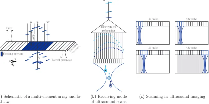
Efficient treatment of diseases needs an accurate diagnosis and understanding of the mechanisms that are involved. In such dynamics, medical imaging is of prime relevance for it is used at several stages in medical processes from detection, to surgery and therapy monitoring. Recent developments in medical imaging reduced treatments invasiveness by allowing physicians to better adapt their procedures. Classical medical imaging techniques such as Magnetic Resonance Imag-ing (MRI), X-rays computerized tomography (CT) or ultrasound scans benefited from a lot of improvements during the end of last century and are now minimally invasive with high sensitiv-ity. Among these techniques, ultrasound is of prime interest for it is cheaper, more compact and wide-spread than the others. Nowadays, several ultrasound scanners can be found in all hospitals and are part of a lot of medical procedures, such as cancer diagnosis and therapy or intraoperative surgical imaging.

It appeared these last few years that, if they now have a good sensitivity (i.e. the ability of detecting a pathology or not), conventional medical imaging techniques often suffer from a lack of specificity (i.e. the ability of distinguishing different pathologies). Current trends in medical imaging are then focused on increasing patient’s specificity. Two approaches are being explored. The first one is molecular imaging and uses biomarkers that specifically interact with a given kind of biological species and increase the associated contrast. The second one is multi-modality that couples different medical imaging techniques in order to overcome detection failures or remove uncertainties. Among these recent developments, multi-waves imaging techniques offer promising outcomes. Such techniques usually couple a specific and poorly resolved modality with a low specificity but highly resolved one in such a way that it is possible to get the best out from the two techniques.

Regarding such challenges, optical contrast has promising potential for it contains both struc-tural (detection of interfaces for instance) and spectral (the chemical nature) information about the biological species it interacts with. The two main current medical optical techniques that can be found in hospitals are microscopy and pulse oximetry. The first one is widely used during surgical procedures for instance by anatomopathologists. In anatomopathology, thin histological sections are used in order to assess the limits of objects to be resected. The second one is used in order to monitor blood oxygenation inside a finger or an ear.

These two biomedical optics techniques give an example of the different kind of information light can bring about tissues: microscopy provides optical-resolution images of cellular structures whereas pulse oximetry provides spectral information about blood in order to measure its

oxy-2 Introduction

genation. On the other hand, these techniques highlight the major issue of optical imaging in biological samples. Microscopy only works on thin and transparent histological sections, pulsed oximetry works on thicker samples but only provides a spatially unresolved measurement of a biological parameter.

These limitations come from multiple light scattering and explain why optical imaging was missing from the list of medical imaging modalities up to now. When propagating inside biolog-ical samples, light is scattered by the structures it encounters so that the information it carries is not interpretable for conventional imaging techniques based on geometrical optics. As a con-sequence, conventional approaches are subject to a compromise between resolution and imaging depth. Optical-resolution techniques must work on ballistic photons that do not experience any scattering events and are limited to shallow depths. On the other hand, techniques working with multiply scattered photons are limited to a resolution equal to one fifth of the sample thickness.

A way of overcoming this difficulty is to couple light and ultrasound. Beside the fact that it is widely used and easy to find, ultrasound is not scattered by biological tissues. The goal of such multi-waves techniques is then to super-resolve optical information coming from deep areas. Acousto-optics is one of these techniques. When propagating through an illuminated area, ultrasound locally modulates light through acousto-optic effect and generates tagged photons. The measurement of those photons power gives information about the light irradiance inside the scattering medium with an ultrasonic resolution.

The detection of tagged photons is very challenging and is studied since mid-90s. Several tech-niques were developed such as camera techtech-niques, self-adaptive interferometry or ultra-narrowband filters. Recent works at the Institut Langevin led to the development of a multi-modal platform coupling conventional ultrasound and acousto-optic imaging that allows adding optical contrast to structural information provided by ultrasound. Such a platform may increase diagnosis accuracy and constitutes the very first step toward clinical imaging. As a consequence, current works are focused on the improvement of the platform in order to address challenges of in vivo imaging.

This manuscript is composed of four distinct parts. The first part aims at introducing the principle of acousto-optic imaging. I will first give the physical properties of light propagation inside biological media and list a few examples of current optical imaging techniques. The idea is to show the main limitations induced by scattering inside biological tissues and how it is usually overcome. I will show that in order to perform proper deep optical imaging, it is necessary to work in the near-infrared (NIR) region and deal with speckle patterns – a random interference pattern. I will then introduce the principle of acousto-optic imaging and the corresponding the-oretical background. The idea is to show that the measurement of tagged photons flux gives a signal proportional to the local light irradiance inside the scattering medium integrated over the ultrasound volume. I will also show that the amount of acousto-optic signal is proportional to the pressure squared. After these quick derivations, I will list several possible ways of filtering tagged photons.

In the second part, I will describe the principle of the multi-modal platform. I will first describe how acousto-optic imaging can be coupled to conventional ultrasound by describing with more details a particular detection scheme based on photorefractive holography. I will show that this kind of detection allows performing interferometry while adapting scattered and reference wave-fronts. I will show that such a method allows overcoming most of the issues induced by speckle patterns. Once this detection scheme is described, I will give more details about our multi-modal platform and first examples of promising proofs of concept. These results will allow to highlight

Introduction 3

the main limitations of the technique that prevent from switching to clinical imaging for now. I will show that current acousto-optic sequences lead to low imaging framerates and that the photorefractive detection is limited by speckle decorrelation in vivo. These two points will be addressed separately in two parts.

In a third part, I will address the problem of low acousto-optic imaging framerate. I will suggest a novel ultrasound sequence based on plane waves and a tomographic reconstruction approach. I will first derive a theoretical framework for the technique in order to assess a few properties and a proper reconstruction method. Among others, I will show that, because of the limited emission angle of linear arrays, the lateral resolution of plane waves images is degraded. On the other hand, I will show that such a sequence leads to increased signal-to-noise ratio (SNR) and allows to decrease the imaging rate up to a factor of about fifty.

In the fourth and last part, I will study the use of spectral holeburning as an ultra-narrowband filter in order to directly measure the flux of tagged photons. Such a technique is not sensitive to speckle decorrelation and makes an interesting candidate for in vivo imaging but was left aside because it works at cryogenic temperatures. The technique as it was suggested is limited by the short lifetime of the hole. I will show that the presence of an external magnetic field increases this lifetime by two orders of magnitude.

Part I

Optical imaging of thick biological

tissues

CHAPTER

1

Optical properties of biological tissues

Table of contents

1.1 Optical contrast in medical imaging . . . 9

1.2 Light-tissues interactions . . . 11

1.2.1 Absorption . . . 12 1.2.2 Scattering . . . 12 Rayleigh scattering . . . 13 Mie scattering . . . 13 1.2.3 The case of biological samples . . . 14 1.3 Light propagation in scattering samples . . . 15

1.3.1 The propagation regimes . . . 16 Ballistic photons . . . 16 Single-scattering . . . 17 Multiple scattering . . . 17 Photons time of flight . . . 18 1.3.2 Of multiply scattered electric field . . . 18 Expression of the multiply scattered electric field . . . 18 Speckle pattern . . . 19 1.4 Optical imaging of scattering samples . . . 20

1.4.1 Ballistic and single-scattered light . . . 20 Microscopy . . . 20 Optical coherence tomography . . . 21 Temporal windowing . . . 22 Imaging from the reflection matrix . . . 23 1.4.2 Working with multiply scattered light . . . 23 Snake-like photons . . . 24 Diffuse optical tomography . . . 24

8 Chapter 1. Optical properties of biological tissues

Imaging with speckle . . . 24 Multi-waves imaging . . . 26 1.5 Summary on optical imaging of scattering media . . . 28

1.1. Optical contrast in medical imaging 9

L

ight can interact with its surroundings in two ways: it can be either absorbed or scattered. Light absorption is related to the chemical nature of the species it encounters and generally carries information about metabolism. Typical absorbing biological species are melanin, blood, proteins or even water [1]. On the other hand, light scattering will occur in the presence of in-terfaces associated with discontinuities of refraction index and will be influenced by anisotropy. Light scattering will generally give information about the structure of tissues. For comparison purpose, PET (Positron Emission Tomography) scans have very specific contrast that gives accu-rate functional information, but need isotopes and usually gives poor information about biological structures [2]. Conventional use of CT scans (X-rays) and ultrasound on the other hand only gives information about biological structures – tissues density for CT, acoustic impedance losses for ultrasound [3, Chapters 2 and 5]. MRI is the only technique that can give both structures [4] and functional imaging [5] but suffers from very high costs and low imaging rates. Recent ad-vances in ultrasound led to efficient Doppler imaging which is able to image blood flows [6] and gave first promising results in functional imaging [7]. Because optical imaging naturally contains both type of contrast, it generally makes a powerful imaging tool. However, it is very important to keep in mind that a medical imaging modality is expected to image entire organs and have to reach depth of several centimetres. This requirement is the major obstacle to the development of optical medical imaging modalities: light is multiply scattered by biological structures beyond 1 mm so that the information it carries is completely lost. In this first chapter, I will describe the properties of light-tissues interaction and show few existing techniques that meet medical imaging requirements, among which is acousto-optic imaging.

1.1 Optical contrast in medical imaging

Over years, optical imaging was thought of as alternative methods to invasive procedures such as surgery. The most straightforward way of performing optical medical imaging is to place a powerful light source behind patient’s organs to image and look at what comes through. Based on this idea, the first optical techniques were optical imaging in transmission. Diaphanography [8], based on the idea of Cutler in 1931 [9], was the first technique of this kind that was developed in clinical applications. It consisted in a transillumination technique with visible or near-infrared (NIR) light used for imaging breast lesions. The concept is based on the fact that blood and tumours absorb NIR light whereas normal breast mostly transmit it as shown on figure 1.1. The main advantage of such a technique was that it was non invasive, non ionizing and easy to set up. Few years later, B. Monsees [10] demonstrated the inefficiency of such transillumination techniques as a diagnosis tool for breast tumours and optical imaging was abandoned in favour of mammography.

The major issue of transillumination techniques such as diaphanography is that the resolution in a multiple-scattering regime is limited to one fifth of the imaging depth [11]. It then rapidly ap-pears that optical techniques fail at imaging early stage tumours of few millimetres sizes. Because of this issue, most of optical clinical techniques are now endoscopic or spectroscopic techniques. The latter techniques are generally used for patients monitoring and take advantage of all

bio-10 Chapter 1. Optical properties of biological tissues

(a) Cutler’s experiment (b) Marshall et al. experiment

Figure 1.1 – Breast imaging through transillumination showing the high absorption of blood and suspicious area compared to normal breast. (a) Figure extracted from [9]. The blood vessels are visible, the black area is an haematoma. (b) Figure extracted from [8]. Clinical application of transil-lumination imaging for detection of breast tumours. The blood vessels are also appearing, the dark area is a carcinoma.

logical chromophores having very different absorption spectra. These techniques usually measure a physiological parameter integrated over the diffused light volume. One of the main techniques in this field is the pulse oximetre in which the oxygen saturation of blood is measured through global light absorption through a finger or an ear [12]. As an other example, light is also widely used in brain studies, as shown in the review of E. M. C. Hillman [13], in order to perform surface functional imaging or in vivo microscopy of exposed cortex.

Human body is mostly composed of water that strongly absorbs non visible light as can be seen on the spectrum extracted from [14] presented on figure 1.2(a). On the other hand, most of the other chromophores (coloured species) that constitute biological tissues strongly absorb in the visible domain. For instance, blood is very absorbing under 600 nm as shown on figure 1.2(b) also extracted from [14]. It comes that biological samples are very absorbing in general, except within a particular region between 600 nm and 1.3 µm. This spectral domain is called the optical therapeutic window and explains why transilluminated biological samples appear red. For medical imaging applications, in which high depths are to be reached, it is thus preferable to work around this wavelength range. People work usually between 700 nm and 900 nm. Recent work of Hong

et al. [15] revealed the existence of a second narrow optical window between 1.3 and 1.4 µm

in which scattering is a bit lower. Exploiting the photoluminescence of single-walled carbon nanotubes, they performed through-scalp and through-skull optical fluorescence brain imaging on living mice. With this approach, they obtained unprecedented dynamic images of brain blood perfusion with a resolution of 10 µm at a depth over 2 mm.

It was recently shown that techniques such as X-rays or conventional ultrasound that image structural alterations in tissues often lack of specificity. In the field of breast cancer imaging for instance, it was shown that mammography has a severe issue of false-positive [16] – breast lesions that are diagnosed as cancerous as they are not – and, more significant for patients, of false-negative [17] – breast lesions that are not detected or diagnosed as not cancerous as they actually are. Some works showed that coupling mammography to Diffuse Optical Tomography (DOT) – that consists in solving an inverse light scattering problem in order to recover images, see section 1.4.2 – allows imaging the haemoglobin concentration in the surroundings of breast lesions [18]. On the other hand, it was shown that optical imaging using fluorescent markers of tumorous tissues provides very specific information similar to what is usually obtained with

1.2. Light-tissues interactions 11

(a) Absorption spectrum of water [14] (b) Absorption spectra of several chro-mophores [14]

High

Low

1: Inferior cerebral vein 2: Superior sagittal sinus 3: Transverse sinus

(c) The optical window around 1.3 and 1.4 µm [15]

Figure 1.2– (a) and (b) Spectra extracted from [14] showing the optical window between 650 nm and 1.3 µm.

(c) Figure extracted from [15] that shows through-scalp and through-skull fluorescence images of the brain vasculature within the NIR regions between 850 nm and 900 nm (left) and 1.3 and 1.4 µm (right)

PET scans, but without the need of radioactive markers. For instance, Koenig et al. developed a whole-body fluorescence optical tomography device based on a principle very close to DOT that allowed imaging lung tumours in mice [19].

If transillumination optical imaging alone turned not to be an efficient technique, these re-cent works showed that optical imaging brings very interesting new information when coupled to structural imaging techniques.

1.2 Light-tissues interactions

Light can interact in two ways with its surroundings. It can be either absorbed or scattered and these two phenomena have a very important influence of how light is measured from the outside. As explained in the previous section, the first optical medical imaging methods were left aside partly because of light scattering that strongly degrades the obtainable resolution. However, a lot of medical applications are still based on light and in particular on light absorption. In this section I suggest to further explore how light can interact with biological tissues in order to introduce the general formalism that will be used in the subsequent manuscript.

12 Chapter 1. Optical properties of biological tissues

Mammogram showing invasive ductal carcinoma

DOT image of hemoglobine concentration (colorbar in μM)

(a) Mammogram and DOT image [18]

Follow up of the lung tumour growth Whole-body tomography of a 14 days-old tumour

(b) Fluorescence image of lung tumours in a mouse [19]

Figure 1.3 – Two examples of recent optical imaging techniques. (a) Figure extracted from [18].

Mammog-raphy coupled with DOT for haemoglobin concentration. The arrows point the tumour out. (b) Figure extracted from [19]. Whole-body fluorescence optical tomography of lung tumours in a mouse.

1.2.1 Absorption

Inside a homogeneous medium, light propagates along a straight line and the loss of energy is given by the Beer-Lambert law. In such a case, light interacts with the different chemical species that absorb photons. Light energy is then dissipated through heat or light emission (fluorescence, phosphorescence). All these phenomena can be characterized through a global absorption coefficient µa, usually given in cm−1, that quantifies the amount of energy lost along with light propagation. This coefficient is defined so that, after propagating over a distance z, the light power flux is given by:

Ψ (z) = Ψ0exp (−µaz) (1.1)

where Ψ0 stands for the input light power flux. This coefficient defines the absorption mean free path which is the average distance a photon can propagate through before experiencing an absorption event. The absorption mean free path is noted la and is defined such as:

la=

1

µa

(1.2) As explained above, absorption is strongly wavelength dependent. In the case of biological tissues, typical absorption coefficients are of the order of 0.5 cm−1 _{within the optical therapeutic} window [20].

1.2.2 Scattering

When propagating inside a homogeneous sample, light energy is dissipated through absorption. In practice, a lot of objects are not homogeneous and constituted of interfaces associated with refrac-tive index changes. These inhomogeneities are responsible for scattering and physics of light at-tenuation can not be reduced to the Beer-Lambert law. Scattering was studied in a lot of books such as the two volumes of A. Ishimaru [21, 22] or the book of Bohren and Huffman [23], I will

1.2. Light-tissues interactions 13

only remind a few properties that will be needed later on. In the whole manuscript, I will only consider elastic scattering in which scattered light has the same frequency as incident light.

Rayleigh scattering

When interacting with a particle, an incident electromagnetic wave induces charges oscillations and local oscillating dipoles. These dipoles radiate and light is re-emitted in an other direction as shown on figure 1.4. When scattering particles are very small compared to the wavelength, the electromagnetic field is homogeneous at the scale of the scatterer. All local dipoles oscillate in-phase and the particle acts as a unique dipole. In far field, the scattering is isotropic in first approximation meaning that each possible emission direction is as likely as the others. This is known as Rayleigh scattering and it can be shown in such a case that the scattered power is strongly wavelength dependent – it decreases as 1/λ4 _{[21, Chapter 2].}

Incident field

Scattered field

Scattering particle

z

x

y

Figure 1.4 – Schematic of the interaction between an incident electromagnetic wave and a single particle.

In case of multiple scattering particles, the phenomenon can be characterized by the typical distance a photon can walk through before being scattered. This distance is called the scattering mean free path and noted ls. From this parameter, it is possible to define a macroscopic coefficient

that quantifies scattering inside the medium light propagates through. This coefficient is noted µs, usually given in cm−1_{, and is related to the statistical distribution of scattering events:}

µs= 1

ls

(1.3) In Rayleigh scattering, each scattering event induces the loss of light previous history (polar-ization, phase and direction). The scattering mean free path is generally function of the kind of scatterers and their concentration in the medium.

Mie scattering

When particles size becomes bigger compared to the wavelength, the electromagnetic field can not be considered as homogeneous over the particle volume anymore. This case is described by the Mie theory [21, Chapter 2] of which Rayleigh scattering is just a particular case. In this case, the scattering is not isotropic anymore and mostly occurs in the forward direction, i.e. directions close to the incident wave one.

14 Chapter 1. Optical properties of biological tissues

The anisotropy of the scattering is defined by an anisotropy coefficient g such as:

g = hcos θi (1.4)

where θ is the angle of scattering as drawn on figure 1.5. This anisotropic scattering preserves light information over several scattering events so one defines a new mean free path called transport mean free path l∗ _{that corresponds to the characteristic distance light can propagate through} before losing the memory of its past history. From this characteristic distance, it is possible to define a corresponding macroscopic coefficient called the reduced scattering coefficient noted µ′ s given in cm−1_. µ′_s= 1 l∗ (1.5)

θ

Incident

photon

Scattered

photon

Figure 1.5– Schematic of the scattering anisotropy.

These new coefficients that quantify the ability of scattering to scramble light information (see figure 1.6) are related to the scattering coefficient through the two relationships:

         µ′ s = µs(1 − g) l∗ ₌ ls 1 − g (1.6) The anisotropy coefficient g varies between 0 and 1. The case g = 0 corresponds to identical contributions of all angles and isotropic scattering. This is what happens in Rayleigh scattering. When g = 1, all photons are scattered in their incident direction and there is no more scattering – as expressed by the reduced scattering coefficient µ′

s = 0. In such a case, light information is never lost and the transport mean free path is infinite. A physical interpretation of the transport mean free path is displayed on figure 1.6.

1.2.3 The case of biological samples

Biological samples are very inhomogeneous media in which all characteristic sizes are found from few nanometres for proteins up to over 10 microns for cells. It leads to very different orders of magnitude in terms of optical properties. A lot of reviews [1, 14, 24] or handbooks [20] can be found that gather a lot of measurements of optical properties of biological samples. Table 1.1 gives the orders of magnitude of optical properties gathered in [1] for human tissues.

1.3. Light propagation in scattering samples 15

l

_s

l*

Preferred scattering direction

Figure 1.6– Schematic of the transport mean free path. It corresponds to the typical distance beyond which

the light loses the memory of its initial direction.

n Refractive index 1.35 – 1.45

µa Absorption coefficient 1 cm−1 – 10 cm−1 at 630 nm

µs Scattering coefficient 100 cm−1 – 500 cm−1 in the visible range

g Anisotropy coefficient _{∼ 0.9}

µ′

s Reduced scattering coefficient 2 cm−1 – 70 cm−1 in the visible range

Table 1.1– Table of the typical optical properties of human tissues taken from [1]

These orders of magnitude concern biological tissues as various as blood, brain or bladder. For instance, typical absorption coefficient of biological tissues are of the order of 1 cm−1 _{or lower} around 800 nm, except for epidermis – of the order of several tens of cm−1 _{– and blood – few} cm−1 _{[20, Chapter 2]. Red blood cells are very anisotropic scatterers in the near-infrared range} for which the anisotropy coefficient is over 0.99 [20, Chapter 2]. Scattering usually decreases as the wavelength is increased [20, Chapter 2], thus explaining the advantage of working further in the infrared [15].

1.3 Light propagation in scattering samples

Multiple-scattering makes deep optical imaging in biological samples challenging. Transmitted photons experience random trajectories that are impossible to deduce from the output direction of these photons. In this section, I will study the propagation of photons inside scattering media and will come out with several propagation regimes: the ballistic regime in which all photons propagate in straight lines, the diffusive regime, in which all photons have random trajectories, and two intermediate regimes, the single-scattered regime and the snake-like regime, also called quasi-ballistic.

16 Chapter 1. Optical properties of biological tissues

1.3.1 The propagation regimes

As explained above, Beer-Lambert law does not completely quantifies light attenuation in the presence of scattering. When light propagates through a scattering sample, it is possible to define two kinds of photons: the ballistic photons that did not experience any scattering events, and the scattered photons that experienced at least one. Three propagation regimes can then be considered depending on the medium thickness L compared to the scattering mean free path. The case L ≪ ls is called ballistic regime. If L ∼ ls, light propagation is in a single-scattering regime.

Finally, the case L ≫ ls is called the multiple-scattering regime. Figure 1.7 shows the different

propagation regime one can experience in a multiply scattering medium.

(1) (2) (3) (4) (5) (0)

Figure 1.7 – Schematic of the different possible propagation regimes in a multiply scattering sample. (0) stands for incident photons. (1) stands for ballistic photons that are transmitted without ex-periencing any scattering event and propagate in straight line. (2) stands for single-scattered photons that experienced only one scattering event. In the multiple scattering regime, two particular cases are represented here: the snake-like photons (3) that appear in anisotropically scattering media and are multiply scattered photons that keep memory of their incident path, and diffused photons (4) and (5) that appear far from the transport mean free path and that correspond to a quasi-isotropic irradiance. (5) represents an example of backscattered photons that are photons scattered back in the direction of the light source, either through single or multiple scattering.

Ballistic photons

The ballistic photons are photons that do not experience any scattering events and propagate in straight lines. The ballistic power flux Ψb decreases exponentially as ballistic photons are absorbed

or scattered. It thus verifies:

Ψb(L) = Ψ0exp [− (µa+ µs) L] (1.7)

The ballistic power flux obeys a generalized Beer-Lambert law that takes scattering into account. The coefficient µa+ µs is called the extinction coefficient and is noted µext. Here, it is to be noted that a photon that went through a scattering event but was re-emitted in the ballistic light direction is not considered as a ballistic photon anymore.

If L ≪ ls, photons do not have time to scatter and only ballistic photons are collected at the

out-put. The medium is not turbid and attenuation is only due to light absorption: optical information is interpretable in terms of geometrical optics. However, in biological samples within the optical

1.3. Light propagation in scattering samples 17

therapeutic window, µs ≫ µa so that the number of ballistic photons decreases as exp (−µsz), where z is the depth inside the medium. It means that ballistic light vanishes over few scattering mean free path, i.e. few hundreds of microns.

Single-scattering

When the size of the scattering medium increases, an intermediate regime appears in which pho-tons only experience a unique scattering event. This particular regime occurs for samples in which L ∼ ls. In this regime, ballistic and scattered photons coexist and multiple scattering

events are neglected.

In the single-scattering regime, all particles are assumed illuminated by the incident field only. Because ballistic light vanishes very fast along with the medium thickness the same happens for single scattered photons. In general, interpretable information for conventional imaging devices is carried by ballistic and single-scattered photons. Reflection-mode imaging devices provide images with single-scattered photons as transmission configurations work with ballistic light.

Multiple scattering

When the scattering medium becomes thick compared to the scattering mean free path L ≫ ls,

multiple scattering events can not be neglected anymore. This is the multiple-scattering regime in which photons have experienced more than one scattering event. In general, scattering is not isotropic so that optical information is preserved over several scattering events. As explained above, this defines the transport mean free path l∗ _{beyond which optical information is scrambled.} For a thickness contained within ls < L < l∗, it is usually considered that single-scattered and

multiply scattered photons coexist. In the multiple-scattering regime, images quality is then driven by the ratio between multiply scattered and ballistic or single-scattered light. The fast decrease of this ratio along with the thickness of the scattering sample is the major imaging depth limitation of optical methods.

Far from the transport mean free path, the luminance is quasi isotropic and there are no ballistic nor single-scattered photons anymore. This regime is called the diffusive regime in which the scattered light power flux obeys a diffusion equation. At a distance r far from l∗_{, the scattered} light irradiance Φs(r) obeys the following equation [21]:

Φs(r) ∝ Ψ0

exph₋q3µa(µa+ µ′s)r

i

r (1.8)

where the proportionality factor is function of the absorption and the reduced scattering coeffi-cients [25]. Far from the transport mean free path, this expression defines the effective extinction coefficient:

µeff =

q

3µa(µa+ µ′s) ∼

q

3µaµ′s in case of strong scattering (1.9)

In strongly anisotropic media, some photons, so-called snake-like or quasi-ballistic photons, are multiply scattered but propagate almost in straight lines. In this intermediary regime, those photons are not strictly speaking ballistic photons for they are multiply scattered, but are not diffused photons for they partially retained their initial direction. The power flux of these photons decreases as: