GARCH Option Pricing Under Skew
Sofiane ABOURA
email: [email protected]
ESSEC Business School
Av. Bernard Hirsch – 95021 Cergy-Pontoise – France
Current version : January 2003
Abstract
This article is an empirical study dedicated to the GARCH Option pricing model of Duan (1995) applied to the FTSE 100 European style options for various maturities. The beauty of this model is to have used the standard GARCH theory in an option perspective and also it is its flexibility to adapt to different rich GARCH specifications. We analyze the valididy of the model given its ability to price one-day ahead out-of-sample call options and also its ability to capture the empirical dynamic of the volatility skew.
We get severe mispricing for deep out-of-the-money and short term call options, which tend to decrease the global performance of the model that is relatively correct. We note that long term skews tend to be more stable across time and strikes, which explains why we had a decreasing pricing bias for longer maturity contracts. We also get that skews tend to deform into smiles as we go toward the expiry date. This model reveals a good ability to capture the change of regime in the implied volatility surface judging from the transformation observed from smiles to skews.
Keywords : GARCH Option models, Monte Carlo simulations, Implied Volatility,Volatility Smile. JEL Classification Codes : C13, G13
1. Introduction
Since the mid seventies, as an alternative to the Black-Scholes (1973) model, a strand of literature devoted to option pricing has emerged with authors that specified the diffusion coefficient being function of the asset price as the CEV model of Cox (1975) or the compound model of Geske (1979). Later on, option theory has been developped under bivariate diffusion processes with authors, such as Hull and White (1987), Wiggins (1987), Scott (1987), Johnson and Shanno (1987) proposing numerical solutions for pricing oprions. Other researchers developed closed-form solutions as Stein and Stein (1991) or Heston (1993) whose model allows for arbitrary correlation between asset returns and volatility. We can also add the universal model of Bakshi, Cao and Chen (1997) very similar to the Heston (1993) but allowing for stochastic interest rate, stochastic volatility and jump diffusion. However, the main limit of these models is that they are difficult to implement.
As an alternative to continuous time models, GARCH framework offered some interesting features. Among them, the fact that current variance is observable since it is a function of past squared shocks and past variance. Thus, estimating the time varying variance is no longer cumbersome as in diffusion processes. The success of GARCH option pricing theory is due both on its flexibility to adapt to every GARCH specifications and also to its connection with the stochastic volatility models. Indeed, Nelson (1990) showed that some univariate GARCH processes can be used to approximate some stochastic volatility bivariate diffusions. Duan (1996) generalized these results through its Unified Theory of GARCH option pricing where he also demonstrated that existing bivariate diffusion models are the limits of the GARCH models and how to use these results for pricing options. Among the authors within this stream of literature, a competitive model was set up by Heston and Nandi (2000). They postulated the same dynamic of Duan (1995) using the NGARCH specification with the slight difference that for obtaining a closed-form solution, the variance is no longer multiplied by the ARCH term but by the asymmetric term. The model is very resembling to the Heston (1993) model in its form, by the inversion of characteristic functions to calculate risk-neutral probabilities. Trevor and Ritchken (1999) developed a lattice based also on the NGARCH model to price both European and American options. Also, the advantage of such an algorithm, is that it can be extended to other GARCH specifications, such as the GJR model or the EGARCH model. In order to avoid exploding trees, they only consider the maximum and minimum variance. Obviously, the more one add the number of states in the algorithm, the more the model
converges to bivariate diffusions. Duan, Gauthier and Simonato (1999) have provided an analytical approximation for the NGARCH process in a form of series expansions. The main advantage of such a model is that they are relatively easy to implement and fast in convergence.
Section 2 presents the option pricing model, section 3 discusses the calibration procedure and gives information on the sampling methodology, section 4 presents and analyses the out-of-sample valuation performance of the model while the section 5 discusses the empirical dynamic of the skew. Section 6 summarizes and concludes.
2. The GARCH option pricing model
We consider usually a one-period returns for the underlying asset since we don’t find generally significant returns influence beyond one day period. Let S be the asset price at t
date t and h be the conditional variance of the logarithmic returns over the a daily interval t
[ ]
t,t+1. Let consider the price process under the physical measure modeled by :( )
f t t t t t t r h h h S S δ λ ε 2 1 ln 1 + − + − = − (1)with r being the risk-free interest rate and f δ the dividend yield. The unit risk premium for
the asset is λ and ε is a standard normal random variable with t εt~N(0,1). Under the same
measure, we consider the following variance process following a non-linear asymmetric GARCH (NGARCH) model as in Engle and Ng [1993] :
(
)
1 1 2 1 -t − − + − + = t t t h h h ω αε γ β (2)where γ is a non-negative parameter likely to capture the negative correlation between returns and volatility correlations. ω, α, β must remain positive to ensure that conditional volatility stays positive. To ensure stationarity of the variance, the parameters should satisfy :
( )
1+γ2 +β<1α . The unconditional variance is given by α
[
1−α( )
1+γ2 −β]
. We note that theBlack-Scholes (1973) model is a particular case of this specification when it reduces to standard homoskedastic log-normal process with α and =0 β . =0
To derive the GARCH option model, Duan (1995) had to apply the risk-neutral valuation defined as the Locally Risk Neutral Valuation Relationship. Under this risk-neutral measure, the price process is given by :
( )
* 1 2 1 ln f t t t t t r h h S S = −δ − + ε − (3)and the variance process is given by :
(
)
1 1 2 *1 -t −( + ) − + − + = t t t h h h ω αε λ γ β (4)where ε being a standard normal random variable with t* εt*~N(0,1). The appearing non
centrality parameter has the following form γ*=λ+γ, but the variance process remains almost
the same. The option model will yield four parameters, ω, α, β and γ while the interest *
rate and the dividend rate are input parameters. By recursion we find easily that the underlying asset price at maturity T is :
(
)
(
)
− − + =∑
∑
+ = + = T t i i i T t i i f t T S r T t - h h S 1 * 1 2 1 exp δ ε (5)Since we cannot derive an analytical approximation of the option price, Monte Carlo simulations are run to estimate a set of N random path of residuals
(
εt*+1,j,...,εT*,j)
withN
j=1,..., . These residuals will be plugged into the last equation to compute the corresponding prices ST,j, given strike prices K , which are in their turn plugged into the risk-neutral
conditional expectation E : * ( ) *
[
max(
,0)
]
K S E e CGARCH = −rf T−t T −This can be approximated by :
( )
[
(
)
]
∑
= − − − = N j j T t T r GARCH S K N e C f 1 , ,0 max 1 (6)The decomposition of the computation can be expressed in two manners whether we use simple Monte Carlo simulation or Empirical Martingale Simulation (EMS) as in Duan and Simonato [1998]. The EMS method that we apply in this study is reputed to accelerate the convergence of Monte Carlo price estimates. The Monte Carlo simulation can be stated as :
) ( ] ) exp[( ) (i S0 r t Z i St = −δ t )] ( 5 . 0 exp[ ) ( ) (i Z 1 i 2 i Zt = t− − σt +σtεt
and for EMS, we must compute :
∑
= − − + − + − = n i t t t t t t t t t i i Z n i i Z i Z 1 2 1 2 1 )] ( 5 . 0 exp[ ) ( 1 )] ( 5 . 0 exp[ ) ( ) ( ε σ σ ε σ σThe next section deals with the calibration procedure of the NGARCH option pricing model along with the sampling methodology.
3. The sampling methodology and the estimation procedure
3.1. The sampling methodology
We consider the period of January 2002 including 22 trading days going from January 2nd to January, 31th. The database only contains closing prices stemming from the FTSE 100 European style purchased at the LIFFE web site and is organized as cross-sectional data. We construct the database using the same number of calls and puts, that is 2310 each. The maturities are the third friday of February, March, June, September and December. For each day of January 2002, we have considered 5 maturities which are for the January 2nd,
[50, 80, 169, 258, 348] days declining until the last day of January to [21, 51, 140, 229, 319] days. The range of strike prices goes from 4225 to 6225 for an average stock price of 5216 with a minimum of 5082 and a maximum of 5411. We compute the implied interest rates and the implied dividend rates from the observed option prices using the method of Shimko [1993] based on the put-call parity, which holds relatively well on the data used in the study. The average implied interest rate is about 3,80% and the implied dividend yield is around 3,73%. As for the average implied volatility, as it is provided by the LIFFE Stock Exchange for the observed period, it is about 20,86% and the ATM volatility is 18,16%.
3.2. The calibration procedure
The procedure for the implied calibration for day N is the following :
Step 1 : we estimate the NGARCH parameters on a FTSE 100 time series of 2001 as a starting
value for the first day of January 2002.
Step 2 : we compute the implied interest rate and implied dividend yield for the day N-1.
Step 3 : using cross-sectional quadratic minimization with all maturities of day N-1, we
estimate the implied NGARCH parameters using the parameters of day N-2 as starting values. The non-linear least squares procedure estimates the values of the NGARCH set of parameters, Θ={ω, α, β,γ , h }, while we set the risk premium parameter λ constant equal to its historical value for simplifying the estimation procedure which minimized the following sum of squared errors :
∑∑
= = = Θ T t N i t i e 1 1 2 , ) ( SSE minWith ei,t representing the difference between the actual price and the theoretical price of
contract i at maturity t . The number of Monte Carlo simulations used is 10000 replications. We noted that 5000 runs produce enough precision to converge to the true prices.
Step 4 : using these implied parameters from day N-1, the implied interest rate and implied
dividend yield from day N-1, the maturity of day N and the current stock price, we compute a stream of residuals using Monte Carlo simulations for the computation of a terminal stock price in order to obtain a NGARCH call price. Note that we could have chosen another GARCH specification, as for example, EGARCH or GJR-GARCH. End of the procedure for computing the call prices for the day N. We ran this procedure for each day of the sample.
4. Empirical tests for the out-of-sample valuation
4.1 Parameter estimates
The study aimed at computing tomorrow’s call prices using each day of January 2002. Table 1 provides average values for each of the NGARCH parameters for the month of January.
Table 1
NGARCH average parameters
Implicit values Historic value
ω α β γ h
λ
5.334E-06 8.759E-02 8.300E-01 0.691 8.670 % 1.262E-02
The volatility computed here is obtained by taking the square root of the NGARCH final variance divided by 252 trading days.
Only the risk premium was set to its historical value computed from the whole year 2001. Typically; the value for the risk premium is weak and has few impact on the option pricing as it is observed in many empirical studies. We found surprisingly a relative weak value of volatility derived from the NGARCH model, but it is also the case in the article of Hsieh and Rithcken (2000).
4.2 Out-of-sample performance
Tables 2, 3 and 4 display the out-of-sample results for the NGARCH option pricing model of Duan (1995) in terms of Pricing Error (PE), Relative Pricing Error (RPE) and Absolute Relative Pricing Error (ARPE). If the PE is defined here as the difference between computed call prices Cˆ and observed pricesi C , the RPE and ARPE are defined as : i
i i i C C C − = ˆ RPE and i i i C C C − = ˆ ARPE
These tables give pricing results per moneyness computed as stock prices divided by strike prices, but also per category of maturities. We therefore display the results by range of maturities, corresponding to February, March, June, September and December. For instance, for the range [50,21], we begin by January 2nd, which has 50 days until maturity, January 3rd, which has 49 days until maturity, etc until January 31th, which has 21 days to maturity. This precise maturity being of course, February, and so on for the other four range of maturity. The last column gives the average results per moneyness whatever is the maturity and the last line gives the average results per maturity whatever is the moneyness. Options with moneyness inferior to 0,94 are denoted DOTM as deep out-the-money options, with moneyness between [0,94; 0,97[ are denoted OTM as out-the-money options, with moneyness belonging to [0,97; 1,00[ and [1,00; 1,03[ are denoted ATM as around-the-money options, with moneyness between [1,03; 1,06[ are denoted ITM as in-the-money options and those with a moneyness superior or equal to 1,06 are denoted DITM as deep in-the-money options.
Table 2
Pricing Error for different moneyness and maturity groups
Maturity in days Moneyness [50,21] [80,51] [169,140] [258,229] [348,319] Average < 0.94 0.608 2.341 12.085 22.495 33.338 14.173 0.94 - 0.97 1.270 4.427 8.388 15.826 20.969 10.176 0.97 - 1.00 -1.075 1.883 3.334 8.096 12.358 4.919 1.00 - 1.03 -4.815 -4.385 -2.604 -0.570 4.240 -1.627 1.03 - 1.06 -7.016 -10.418 -8.566 -7.167 -3.780 -7.389 ≥ 1.06 -4.748 -16.548 -18.066 -19.874 -19.479 -15.743 All options -2.322 -5.703 -2.299 1.871 7.123 -0.266
The pricing errors are computed as the difference between the computed call price and the observed call price.
We first see that for PE measure, in average, the best out-of-sample fit is for ATM call options while far from the money contracts seems to suffer from a severe mispricing. As the maturity increases, the mispricing for DITM and DOTM options is being worse. The negative
values show that prices are under-estimated, which is the case for ITM options and for most of ATM options.
Table 3
Relative Pricing Error or different moneyness and maturity groups
Maturity in days Moneyness [50,21] [80,51] [169,140] [258,229] [348,319] Average < 0.94 0.045 0.719 0.472 0.335 0.282 0.371 0.94 - 0.97 0.015 0.110 0.063 0.075 0.072 0.067 0.97 - 1.00 -0.022 0.022 0.017 0.028 0.034 0.016 1.00 - 1.03 -0.037 -0.024 -0.008 -0.001 0.009 -0.012 1.03 - 1.06 -0.029 -0.039 -0.022 -0.015 -0.007 -0.022 ≥ 1.06 -0.009 -0.028 -0.026 -0.025 -0.022 -0.022 All options -0.009 0.186 0.161 0.117 0.105 0.112
The pricing errors are computed as the difference between the computed call price and the observed call price.
We also get the best pricing for ATM options but we observe that as in Table 2, the mispricing of these options is increasing as we move towards short term contracts. Note that ATM contracts are underestimated for options with maturity less than one year. We see that, in average, the worse mispricing is systematically produced by DOTM options. If we get away these DOTM contrats, we would have a pricing precision that would be much more improved.
Table 4
Absolute Relative Pricing Error for different moneyness and maturity groups
Maturity in days Moneyness [50,21] [80,51] [169,140] [258,229] [348,319] Average < 0.94 0.788 0.783 0.472 0.335 0.282 0.532 0.94 - 0.97 0.192 0.127 0.066 0.076 0.075 0.107 0.97 - 1.00 0.104 0.049 0.030 0.034 0.041 0.052 1.00 - 1.03 0.054 0.034 0.020 0.020 0.026 0.031 1.03 - 1.06 0.035 0.039 0.025 0.022 0.021 0.028 ≥ 1.06 0.010 0.028 0.026 0.027 0.026 0.023 All options 0.199 0.249 0.183 0.138 0.120 0.178
The pricing errors are computed as the difference between the computed call price and the observed call price.
We also get a severe mispricing for DOTM options which is almost five times worse than other moneyness. Thus, the more we move towards DOTM contracts, the more the pricing biais is increased. We note that the pricing precision is a function of the maturity. The more the maturity increases, the more the bias pricing is reduced.
5. The empirical dynamic of the skew
Figure 1 displays the skews generated by the Duan (1995) ‘s model for respectively, the first day (Figure 1a) and last day (Figure 1b) of the sample. It shows the observed deformation of the implied volatility surface during January 2002.The implied volatilities in the vertical axes are computed by equating the Black-Scholes (1973) formula to the prices computed by the NGARCH option pricing model. These theoretical prices are obtained from an out-the-sample fit. In the horizontal axis, we displayed the strike prices. Additional Figures are presented in appendice. Figure 1a Figure 1b 0,17 0,19 0,21 0,23 0,25 0,27 4225 4425 4625 4825 5025 5225 5425 5625 5825 6025 6225
49 days 79 days 168 days
257 days 347 days 0,14 0,16 0,18 0,20 0,22 0,24 4225 4425 4625 4825 5025 5225 5425 5625 5825 6025 6225
21 days 51 days 140 days
229 days 319 days
Figure 1 – Skews computed from an out -the-sample valuation on January, 2nd 2002
Figure 1a shows almost linear skews per maturities for the first day of the sample. We see that for ITM calls, the slope of the skew is all the more high that the maturity is short. Once, we arrive to the ATM options around 5375-5425 points, the scheme is reversed with the difference that the slope coefficients are very tight. This center point has a pivotal role since it reverse the order of the skews.
For the last day of the sample, in Figure 1b, skews are no longer linear except for long maturities (229 days and 319 days). The more the maturity is short, the more the curvature of the smile around the money is high. For DITM calls, i.e, from 4225 to 4725, we get a reverse smile for shorter maturities. Note that this model allows for both skew and smile patterns which is quite important to capture all the features of the deformation of the true implied volatility surface.
We also carried out a simple position analysis with skews re-computed from an in-the-sample fit (i.e, implied volatilities were obtained from an in-the-sample valuation) to get theoretical prices closer to true prices. We found that for the more we increase in maturity, the more the rank between skews is stable, day after day. This should mean that it is easier to predict long term implied volatilities rather than short term. For the group of maturities [348,319], the number of shifts between ranks for the whole month is 61, for the group [258,229] it is 76, for the group [169,140] it is 142, for the group [80,51] it is 239 and for the last group [50,21] it has slightly decreased to 214. This is certainly due to the growing uncertaincy in the approach of the expiry date. This can explains why the model succeed in pricing contracts with longuest maturities since long term implied volatilities are more stable across time.
6. Conclusion
This article is an empirical study of the GARCH Option pricing model developped by Duan (1995). This model is implemented on the FTSE 100 European style options for five range of maturities. Using the NGARCH specification, we explain our implied calibration procedure and apply it to compute one-day ahead out-of-sample call option prices for January 2002.
Severe mispricing was found for deep out-the-money options which worsen the global performance of the model that is relatively correct judging from the pricing error. The best fit is made for at-the-money options, which is generally the case of many models, even the Black-Scholes (1973) model.
We note that the pricing bias is decreasing with the maturity, which means that this model succeed in pricing long term options, which is consistent with our analysis that long term skews are more stable in time and thus more predictable. However, the global performance remains good regarding the srtong stability of the model.
The model of Duan (1995) generates almost downward linear skews for long maturities. We observed that as we move closed to the expiry date, we get a deformation of the skews that transform into smiles for around the money options. Therefore, the ability of the model to capture the deformation of the skew dynamic through time shows that this model is sensitive to the change of regime in the implied volatility surface.
References
Black, F. & Scholes, M., (1973), The pricing of options and corporate liabilities, Journal of
Political Economy, 81, 637-659.
Blair, B.J., Poon, S.H., & Taylor, S.J., (2001), Forecasting S&P100 volatility: The incremental information content of implied volatilities and high frequency index returns,
Journal of Econometrics, 105, 5-26.
Bollerslev, T., Chou, R.Y., & Kroner, K.F., (1992), ARCH modeling in finance: A selective review of the theory and empirical evidence, Journal of Econometrics, 52, 5-59. Christensen, B.J. & Prabhala, N.R., (1998), The relation between implied and realized
volatility, Journal of Financial Economics, 50, 125-150.
Day, T.E. & Lewis, C.M., (1992), Stock market volatility and informational content of stock index options, Journal of Econometrics, 52, 267-287.
Dimson, E. & Marsh, M., (1990), Volatility forecasting without data-snooping, Journal of
Banking and Finance 14, 399-421.
Ding, Z., Granger, C.W.J., & Engle R., (1993) A long memory property of stock market returns and a new model, Journal of Empirical Finance, 1, 83-106.
Duan, J.C. (1995), The GARCH option pricing model, Mathematical Finance, 5, 13-32. Duan, J.C. (1996), Cracking the smile, RISK, 9, 55-59.
Duan, J.C. & Simonato, J.G., (1998a), Empirical martingale simulation for asset prices,
Management Science, 44, 1218-1233.
Duan, J.C. & Simonato, J.G., (1998b), American option pricing under GARCH by a Markov chain approximation, Department of Finance, Hong Kong University of Science and Technology, Working Paper.
Duan, J.C., Gauthier, G., & Simonato, J.G., (1998), An analytical approximation for the
GARCH option pricing model, Department of Finance, Hong Kong University of Science and Technology, Working Paper.
Duan, J.C. (1999), Conditional fat-tailed distributions and the volatility smile in options, Department of Finance, Hong Kong University of Science and Technology, Working Paper.
Duan, J.C., Gauthier, G., & Simonato, J.G., (2001), Asymptotic distribution of the empirical martingale simulation option price estimator, to appear in Management Science.
Dumas, B., Fleming, J., & Whaley, R.E., (1998), Implied volatility functions: empirical tests,
The Journal of Finance, 53, 2059-2106.
Engle, R.F., & Ng, V., (1993), Measuring and testing the impact of news on volatility,
Journal of Finance, 48, 1749-78.
Franses, P.H. & Van Dijk, D., (1995), Forecasting stock market volatility using (non-linear) GARCH models, Journal of Forecasting, 15, 229-235.
Fleming, J., Ostdiek, B., & Whaley, R.E., (1995), Predicting stock market volatility: a new measure, Journal of Futures Markets, 15, 229-235.
Fleming, J. (1998), The quality of market volatility forecasts implied by S&P100 index option prices, Journal of Empirical Finance, 5, 317-345.
Glosten, L.R., Jagannathan, R., & Runkle, D.E., (1993), On the relation between the expected value and the volatility of the nominal excess return on stocks, Journal of Finance, 48, 1779-1801.
Heston, S.L. (1993), A closed-form solution for options with stochastic volatility with
applications to bond and currency options, The Review of Financial Studies, 6, 327-343. Heston, S.L. & Nandi, S., (2000), A closed-form GARCH option valuation model, The
Review of Financial Studies, 3, 585-625.
volatilities, Journal of Financial and Quantitative Analysis, 29, 31-56.
Hsieh, K.C. & Rithcken, P., (2000), An empirical comparison of GARCH option pricing models, working paper, Case Western Reserve University.
Hull, J. & White, A., (1987), The pricing of options on assets with stochastic volatilities,
Journal of Finance 42, 281-300.
Jorion, P. (1995), Predicting volatility in the foreign exchange market, Journal of Finance, 50, 507-528.
Kallsen, J. & Taqqu, M., (1998), Option pricing in ARCH-type models, Mathematical
Finance, 8, 13-26.
Naik, V. & Lee, M.H., (1990), General equilibrium pricing of options on the market portfolio with discontinuous returns, Review of Financial Studies, 3, 493-522.
Nelson, D. (1991), Conditional heteroskedasticity in asset returns: a new approach,
Econometrica, 59, 347-370.
Nelson, D. (1992), Filtering and forecasting with misspecified ARCH models I: getting the right variance with the wrong model, Journal of Econometrics, 52, 61-90.
Nelson, D. & Foster, D.P., (1995), Filtering and forecasting with misspecified ARCH models II: making the right forecast with the wrong model, Journal of Econometrics, 67, 303-335.
Ritchken, P. & Trevor, R., (1999), Pricing options under generalized GARCH and stochastic volatility processes, Journal of Finance, 54, 377-402.
Shimko, D. (1993), Bounds of probability, RISK, 6, 33-37.
Stein, E. & Stein, J., (1991), Stock price distributions with stochastic volatility: an analytic approach, Review of Financial Studies, 4, 727-752.
Wiggins, J. (1987), Option values under stochastic volatility: theory and empirical estimates,
Journal of Financial Economics, 19, 351-372.
Appendix
The following graphics display the volatility skews per range of maturities in days : long term maturities [229; 258] and [140; 169], middle term maturities [51; 80] and short term maturities [21-50]. The vertical axis gives the equivalent Black-Scholes (1973) implied volatilities obtained by inverting the formula to each theoretical prices generated by the NGARCH option pricing model as in Figure 1. The horizontal axis shows the range of strike prices from 4225 to 6225.
Figure 2a Figure 2b 0,17 0,19 0,21 0,23 0,25 4225 4425 4625 4825 5025 5225 5425 5625 5825 6025 6225 258 257 256 253 252 251 250 249 246 245 244 243 242 239 238 237 236 235 232 231 230 229 0,17 0,19 0,21 0,23 0,25 4225 4425 4625 4825 5025 5225 5425 5625 5825 6025 6225 169 168 167 164 163 162 161 160 157 156 155 154 153 150 149 148 147 146 143 142 141 140
Figure 2 – Skews computed from an out -the-sample valuation on January 31th 2002
Figure 2a displays the skews for very long maturity contracts. We get very tightened skews with a maximum volatility level around 22 and 25%. These skews are almost linear with decreasing strike prices. Figure 2b shows the deformation process that increases the convexity of the skews generated by short term options.
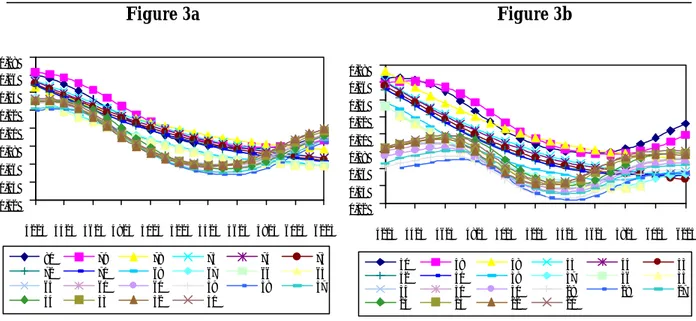
Figure 3a Figure 3b 0,12 0,14 0,16 0,18 0,20 0,22 0,24 0,26 0,28 4225 4425 4625 4825 5025 5225 5425 5625 5825 6025 6225 80 79 78 75 74 73 72 71 68 67 66 65 64 61 60 59 58 57 54 53 52 51 0,12 0,14 0,16 0,18 0,20 0,22 0,24 0,26 0,28 4225 4425 4625 4825 5025 5225 5425 5625 5825 6025 6225 50 49 48 45 44 43 42 41 38 37 36 35 34 31 30 29 28 27 24 23 22 21
Figure 5 – Skews computed from an out -the-sample valuation from January 2nd to January 31th 2002
Figure 3 shows the skews for the middle and short term contracts. Figure 3a displays two groups of skews, one remaining almost linear with strike prices and the other one, transforming into smile patterns. Figure 3b reveals that almost all the skews have been transformed into smiles with a bottom level for ATM options around 5425. The distinction between one month and two months maturities is obvious over all for ITM call options since
the two month maturity group has a maximum volatility around 27% while the one month maturity group begins with a maximum volatility around 19%. We see that the NGARCH option pricing model is able to capture the skew deformation into smiles pattern which makes it more sensitive to the change of regimes that occurred in the implied volatility dynamic.