cut problems
Hassene Aissi, Cristina Bazgan, and Daniel Vanderpooten
LAMSADE, Universit´e Paris-Dauphine, France {aissi,bazgan,vdp}@lamsade.dauphine.fr
Abstract. This paper investigates the complexity of the min-max and min-max regret versions of the s − t min cut and min cut problems. Even if the underlying problems are closely related and both polynomial, we show that the complexity of their min-max and min-max regret ver-sions, for a constant number of scenarios, are quite contrasted since they are respectively strongly NP -hard and polynomial. Thus, we exhibit the first polynomial problem, s − t min cut, whose min-max (regret) versions are strongly NP -hard. Also, min cut is one of the few polynomial prob-lems whose min-max (regret) versions remain polynomial. However, these versions become strongly NP -hard for a non constant number of scenar-ios. In the interval data case, min-max versions are trivially polynomial. Moreover, for min-max regret versions, we obtain the same contrasted result as for a constant number of scenarios: min-max regret s − t cut is strongly NP -hard whereas min-max regret cut is polynomial.
Keywords: min-max, min-max regret, complexity, min cut, s − t min cut.
1
Introduction
The definition of an instance of a combinatorial optimization problem requires to specify parameters, in particular objective function coefficients, which may be uncertain or imprecise. Uncertainty/imprecision can be structured through the concept of scenario which corresponds to an assignment of plausible values to model parameters. Each scenario s can be represented as a vector in IRm
where m is the number of relevant numerical parameters. Kouvelis and Yu [7] proposed the min-max and min-max regret criteria, stemming from decision theory, to construct solutions hedging against parameters variations. In min-max optimization, the aim is to find a solution having the best worst case value across all scenarios. In min-max regret problem, it is required to find a feasible solution minimizing the maximum deviation, over all possible scenarios, of the value of the solution from the optimal value of the corresponding scenario. Two natural ways of describing the set of all possible scenarios S have been considered
⋆This work has been partially funded by grant CNRS/CGRI-FNRS number 18227.
The second author was partially supported by the ACI S´ecurit´e Informatique grant-TADORNE project 2004.
in the literature. In the discrete scenario case, S is described explicitly by the list of all vectors s ∈ S. In this case, we distinguish situations where the number of scenarios is constant from those where the number of scenarios is non constant. In the interval data case, each numerical parameter can take any value between a lower and upper bound, independently of the values of the other parameters. Thus, in this case, S is the cartesian product of the intervals of uncertainty for the parameters.
Complexity of the min-max (regret) versions has been studied extensively during the last decade. In the discrete scenario case, this complexity was inves-tigated for several combinatorial optimization problems in [7]. In general, these versions are shown to be harder than the classical versions. For a constant num-ber of scenarios, pseudo-polynomial algorithms, based on dynamic programming, are given in [7] for the min-max (regret) versions of shortest path, knapsack and minimum spanning tree for grid graphs. The latter result is extended to general graphs in [1]. However, up to now, no polynomial problem was known to have min-max (regret) versions which are strongly NP -hard. When the number of scenarios is not constant, these versions usually become strongly NP -hard, even if the underlying problem is polynomial. In the interval data case, extensive re-search has been devoted for studying the complexity of min-max regret versions of various optimization problems including shortest path [5], minimum spanning tree [4, 5] and assignment [2].
We investigate in this paper the complexity of min-max (regret) versions of two closely related polynomial problems, min cut and s − t min cut. Quite interestingly, for a constant number of scenarios, the complexity status of these problems is widely contrasted. More precisely, min-max (regret) versions of min cut are polynomial whereas min-max (regret) versions of s−t min cut are strongly NP-hard even for two scenarios. We also prove that for a non constant number of scenarios, min-max (regret) min cut become strongly NP -hard.
In the interval data case, min-max versions are trivially polynomial. More-over, for min-max regret versions, we obtain the same contrasted result as for a constant number of scenarios: min-max regret s − t cut is strongly NP -hard whereas min-max regret cut is polynomial.
After presenting preliminary concepts (Section 2), we investigate the com-plexity of min-max (regret) versions of min cut and s − t min cut in the discrete scenario case (Section 3), and in the interval data case (Section 4).
2
Preliminaries
Let us consider an instance of a 0-1 minimization problem Q with a linear ob-jective function defined as:
½
minPmi=1cixi ci∈ N
x∈ X ⊂ {0, 1}m
This class encompasses a large variety of classical combinatorial problems, some of which are polynomial-time solvable (shortest path problem, minimum span-ning tree, . . . ) and others are NP -difficult (knapsack, set covering, . . . ).
In the discrete scenario case, the min-max (regret) version associated to Q has as input a finite set of scenarios S where each scenario s ∈ S is represented by a vector (cs
1, . . . , csm). In the interval data case, each coefficient ci can take
any value in the interval [ci, ci]. In this case, the scenario set S is the cartesian
product of the intervals [ci, ci], i = 1, . . . , m.
We denote by val(x, s) = Pmi=1cs
ixi the value of solution x ∈ X under
scenario s ∈ S, by x∗
s an optimal solution under scenario s, and by val ∗ s =
val(x∗
s, s) the optimal value under the scenario s.
The min-max optimization problem corresponding to Q, denoted by Min-Max Q, consists of finding a solution x having the best worst case value across all scenarios, which can be stated as:
min
x∈Xmaxs∈S val(x, s)
This version is denoted by Discrete Min-Max Q in the discrete scenario case, and by Interval Min-Max Q in the interval data case.
Given a solution x ∈ X, its regret, R(x, s), under scenario s ∈ S is defined as R(x, s) = val(x, s) − val∗
s. The maximum regret Rmax(x) of solution x is then
defined as Rmax(x) = maxs∈SR(x, s).
The min-max regret optimization problem corresponding to Q, denoted by Min-Max Regret Q, consists of finding a solution x minimizing the maximum regret Rmax(x) which can be stated as:
min
x∈XRmax(x) = minx∈Xmaxs∈S{val(x, s) − val ∗ s}
This version is denoted by Discrete Min-Max Regret Q in the discrete scenario case, and by Interval Min-Max Regret Q in the interval data case. In the interval data case, for a solution x ∈ X, we denote by c−(x) the worst
scenario associated to x, where c−
i (x) = ci if xi = 1 and c−i (x) = ci if xi = 0,
i= 1, . . . , m. Then we can establish easily that Rmax(x) = R(x, c−(x)), as shown
e.g. in [9] in the specific context of the minimum spanning tree problem. In this paper, we focus on the min-max (regret) versions of the two following cut problems:
Min Cut
Input: A connected graph G = (V, E) with weight wij associated with each
edge (i, j) ∈ E.
Output: A cut in G, that is a partition of V into two sets, of minimum value. s− t Min Cut
Input: A connected graph G = (V, E) with weight wij associated with each
edge (i, j) ∈ E, and two specified vertices s, t ∈ V .
Output: An s − t cut in G, that is a partition of V into two sets V1 and V2,
with s ∈ V1 and t ∈ V2, of minimum value.
In order to prove our complexity results we use the two following problems proved strongly NP -hard in [6].
Min Bisection
Input: A graph G = (V, E) with an even number of vertices.
Output: A bisection in G, that is a partition of V into two equal cardinality sets, of minimum value.
s− t Min Bisection
Input: A graph G = (V, E) with an even number of vertices, and two specified vertices s, t ∈ V .
Output: An s − t bisection in G, that is a partition of V = V1∪ V2 such that
s∈ V1, t ∈ V2, and |V1| = |V2|, of minimum value.
3
Discrete scenarios case
We show in this section the first polynomial-time solvable problem, s − t Min Cut, which becomes strongly NP -hard when considering its max or min-max regret version.
Min-max cut was proved polynomially solvable for a constant number of scenarios [3]. We show that min-max regret cut also remains polynomial for a constant number of scenarios. When the number of scenarios is not constant, min-max (regret) versions become strongly NP -hard.
3.1 s−t min cut
In order to prove these results, we construct polynomial reductions from the decision version of Min Bisection.
Theorem 1. Discrete Min-Max (Regret) s − t Cut are strongly NP-hard even for two scenarios.
Proof. Consider an instance G = (V, E) of Min Bisection with |V | = 2n, and a positive integer v. We construct an instance eG= ( eV , eE) of Discrete Min-Max s− t Cut with the scenario set S = {s1, s2}. The node set is eV = V ∪ {s, t}
where s and t correspond to a source and a sink respectively. The edge set e
E = E ∪ {(s, i) : i ∈ V } ∪ {(i, t) : i ∈ V }. Edge weights in scenarios s1 and s2
are assigned for each edge (i, j) ∈ eE as follows:
w1ij= 1 if (i, j) ∈ E n2+ 1 if i = s or j = s 0 if i = t or j = t and wij2 = 1 if (i, j) ∈ E 0 if i = s or j = s n2+ 1 if i = t or j = t We claim that there exists a bisection C in G of value at most v if and only if there exists an s − t cut eCin eGwith max{val( eC, s1), val( eC, s2)} ≤ v + (n2+ 1)n.
⇒ Consider a bisection C = (V1, V2) of value x ≤ v. We construct an s − t cut
e
C = ( eV1, eV2) where eV1 = V1∪ {s}, and eV2 = V2∪ {t}. Consequently, we have
⇐ Consider now an s−t cut eC= ( eV1, eV2) verifying max{val( eC, s1), val( eC, s2)} ≤
v+ (n2+ 1)n. Let V
1 = eV1\ {s} and V2 = eV2\ {t}. We have by construction
val( eC, s1) = y+|V2|(n2+1) and val( eC, s2) = y+|V1|(n2+1), where y is the
num-ber of edges from E that have one endpoint in V1and one endpoint in V2. Suppose
that |V1| = n + z and |V2| = n − z, z ≥ 0. Then val( eC, s1) = y + (n2+ 1)n −
z(n2+1), val( eC, s
2) = y+(n2+1)n+z(n2+1) and max{val( eC, s1), val( eC, s2)} =
y+ (n2+ 1)n + z(n2+ 1) ≤ v + (n2+ 1)n. Since v ≤ n2we have z = 0 and thus
|V1| = |V2| = n and y ≤ v.
In order to prove the result for the min-max regret version, we use exactly the same graph eG= ( eV , eE). Let C∗
i denote the optimal solution in scenario si,
i= 1, 2. We have C∗ 1 = ( eV\ {t}, {t}) and C ∗ 2 = ({s}, eV \ {s}) with val(C ∗ 1, s1) = val(C∗
2, s2) = 0. Therefore, there exists a bisection in G of value at most v if and
only if there exists an s − t cut eC in eGwith Rmax( eC) ≤ v + (n2+ 1)n. 2
3.2 Min cut
Armon and Zwick [3] constructed a polynomial-time algorithm for Discrete Min-Max Cut, in the case of a constant number of scenarios, based essentially on the result of Nagamochi, Nishimura and Ibaraki [8] for computing all α-approximate cuts in time O(m2n+ mn2α). A cut C in a graph G is called an
α-approximate cut if val(C) ≤ α opt, where opt is the value of a minimum cut in G.
Theorem 2 ([3]). Discrete Min-Max Cut is solvable in polynomial time for a constant number of scenarios.
In a graph on n vertices and m edges and with k scenarios, Armon and Zwick’s algorithm [3] constructs an optimal solution in O(mn2k).
We show in the following that this algorithm can be modified in order to obtain a polynomial-time algorithm for Discrete Min-Max Regret Cut. Theorem 3. Discrete Min-Max Regret Cut is solvable in polynomial time for a constant number of scenarios.
Proof. Consider an instance I of the problem given by graph G = (V, E) on n vertices and m edges and a set of k scenarios S such that each edge (i, j) ∈ E has a weight ws
ij in scenario s. We construct, as before, an instance I
′ of Min
Cut on the same graph, where w′ ij =
P
s∈Sw s
ij. The algorithm consists firstly
of computing all k-approximate cuts and secondly of choosing among these cuts one with a minimum maximum regret.
The running time of the algorithm is O(mn2k).
We prove now the correctness of the algorithm. Let C∗ be an optimal
min-max regret cut in G. We show that for any cut C of G, we have val′(C∗) ≤
kval′(C), where val′(C) is the value of cut C in I′. In fact,
val′ (C∗ ) =X s∈S val(C∗ , s) =X s∈S (val(C∗ , s) − val∗ s) + X s∈S val∗ s ≤
kmax s∈S{val(C ∗ , s) − val∗ s} + X s∈S val∗ s ≤ k max s∈S{val(C, s) − val ∗ s)} + X s∈S val∗ s≤ kX s∈S (val(C, s) − val∗ s) + X s∈S val∗ s= k X s∈S val(C, s) − (k − 1)X s∈S val∗ s≤ kval ′ (C) In particular, if C is a minimum cut in I′, we obtain val′(C∗) ≤ kopt(I′).
Thus all optimal solutions to Discrete Min-Max Regret Cut are among the k-approximate cuts in I′.
2 The algorithms described above to solve Discrete Min-Max (Regret) Cut are exponential in k. We prove in the following that when k is not constant, both problems become strongly NP -hard.
Theorem 4. Discrete Min-Max (Regret) Cut are strongly NP-hard for a non constant number of scenarios.
Proof. We use a reduction from Min Bisection. Consider an instance G = (V, E) of Min Bisection with V = {1, . . . , 2n}, and a positive integer v. We construct an instance eG= ( eV , eE) of Discrete Min-Max Cut with a scenario set S of size 2n. The node set is eV = V ∪ {1′
, . . . ,2n′} ∪ {1′′
, . . . ,2n′′}. The edge
set eE= E ∪ {(i′
, j′) : i, j = 1, . . . , 2n} ∪ {(i, i′), (i′
, i′′) : i = 1, . . . , 2n}. Scenario
set S corresponds to nodes of G. The weights of the edges in any scenario si∈ S
are defined as follows: wi
hj = 1 for all (h, j) ∈ E; wii′j′ = n2, for j = 1, . . . , 2n;
wi
h′j′ = 0 for h 6= i and j 6= i; wiii′ = wii′i′′ = n3+ n2+ 1; wijj′ = wji′j′′ = 0, for
j6= i.
We claim that there exists a bisection C in G of value at most v if and only if there is a cut eC in eGwith maxs∈Sval( eC, s) ≤ n3+ v.
⇒ Consider a bisection C = (V1, V2) in G of value x ≤ v. We construct a cut
e
C= ( eV1, eV2) in eGwhere eV1= V1∪ {i′, i′′: i ∈ V1} and eV2= V2∪ {i′, i′′: i ∈ V2}.
For any scenario s ∈ S, we have val( eC, s) ≤ n3+ v and thus maxs∈Sval( eC, s) ≤
n3+ v.
⇐ Consider now a cut eC = ( eV1, eV2) in eGsuch that maxs∈Sval( eC, s) ≤ n3+ v.
Cut eC does not contain any edge (i, i′) or (i′
, i′′) for some i = 1, . . . , 2n, since
otherwise, we have maxs∈Sval( eC, s) ≥ n3+ n2+ 1 > n3+ v. Denote by Vi, for
i= 1, 2, the restriction of eVi to the vertices of V . Suppose now that |V1| < |V2|,
then for any scenario si such that i ∈ V1 we have val( eC, si) ≥ (n + 1)n2+ 1 >
n3+ v . Thus, we have necessarily |V1| = |V2| and the value of the bisection
(V1, V2) is at most v.
In order to prove the result for the min-max regret version, we use exactly the same graph eG = ( eV , eE). Notice that, for any scenario si ∈ S, cut Ci∗ =
({j′′}, e
V \ {j′′}) for some j 6= i is a minimum cut in scenario s
i, with value 0.
Therefore, there exists a bisection in G of value at most v if and only if there exists a cut eCin eGwith Rmax( eC) ≤ n3+ v. 2
Observe that in the previous proof we used the same graph eGboth for the min-max and min-max regret versions. Actually, a slightly simpler proof can be
obtained, for the min-max part, considering only the subgraph of eG induced by eV \ {1′′
, . . . ,2n′′
}. Vertex subset {1′′
, . . . ,2n′′
} is necessary, for the min-max regret part, to ensure the existence of minimum cuts of value 0 for each scenario.
4
Interval data case
We first state the polynomiality of the min-max cut problems (Section 4.1), then we establish the strong NP -hardness of Interval Min-Max Regret s − t Cut (Section 4.2) and the polynomiality of Interval Min-Max Regret Cut (Section 4.2).
4.1 Min-max versions
In the interval data case, the min-max version of a minimization problem corre-sponds to solving this problem in the worst-case scenario defined by the upper bounds of all intervals. Therefore, a minimization problem and its min-max ver-sion have the same complexity. Interval Min-Max s − t Cut and Interval Min-Max Cut are thus polynomial-time solvable.
4.2 Min-max regret versions
When the number u ≤ m of uncertain/imprecise parameters, corresponding to non-degenerate intervals, is small enough, then the problem becomes polynomial. More precisely, as shown by Averbakh and Lebedev [5] for general networks problems solvable in polynomial time, if u is fixed or bounded by the logarithm of a polynomial function of m, then the min-max regret version is also solvable in polynomial time (based on the fact that an optimal solution for the min-max regret version corresponds to one of the optimal solutions for the 2u extreme
scenarios, where extreme scenarios have values on each edge corresponding to either the lower or upper bound of its interval). This clearly applies to the s − t min cut and min cut problems.
s−t min cut
We show now that Interval MinMax Regret s − t Cut is strongly NP -hard. For this purpose, we construct a reduction from the decision version of s− t Min Bisection.
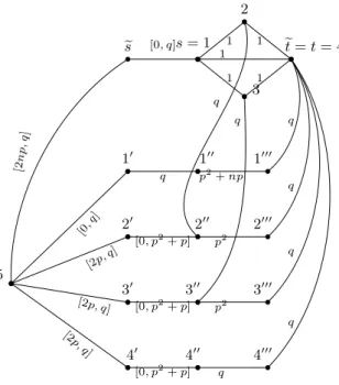
Theorem 5. Interval Min-Max Regret s − t Cut is strongly NP-hard. Proof. Consider G = (V, E) an instance of s − t Min Bisection with |V | = 2n, where V = {s = 1, . . . , t = 2n}. We construct from G an instance eG= ( eV , eE) of Interval Min-Max Regret s − t Cut as illustrated in Figure 1. The vertex set is eV = V ∪ {1′ , . . . ,2n′} ∪{1′′ , . . . ,2n′′} ∪{1′′′ , . . . ,2n′′′ } ∪{es, 2n + 1}, and et= t.
The edge set is eE = E ∪ {(i′ , i′′ ), (i′′ , i′′′ ) : i = 1, . . . , 2n} ∪ {(i, i′′ ) : i = 2, . . . , 2n − 1} ∪ {(2n + 1, i′ ) : i = 1, . . . , 2n} ∪{(i′′′ , t) : i = 1, . . . , 2n} ∪ {(es, 2n + 1), (es, s)}.
Let p and q verifying, respectively, p > n2 and q > 4n(p + 1)2. The weights
are defined as follows :
– wij= wij = 1, for all (i, j) ∈ E;
– wi′i′′= ½ qfor i = 1 0 otherwise and wi′i′′= ½ q for i = 1 p2+ p otherwise – wi′′i′′′ = wi′′i′′′= p2+ np for i = 1 p2 for i = 2, . . . , 2n − 1 q for i = 2n – wii′′= wii′′= q, for i = 2, . . . , 2n − 1; – w(2n+1)i′ = ½ 0 for i = 1
2p otherwise and w(2n+1)i′= q, for i = 1, . . . , 2n; – wi′′′t= wi′′′t= q, for i = 1, . . . , 2n;
– wes(2n+1)= 2np and wes(2n+1)= q;
– wess= 0 and wess= q.
Clearly this transformation can be obtained in polynomial time. We first establish the following property.
For any es − et cut eC = ( eV1, eV2) in eG not including any edge (i, j) ∈ eE with
wij = q, a minimum es − et cut Cw∗−( eC)in, w−( eC), the worst scenario associated
to eC, has value val(C∗ w−( eC), w
−( eC)) = 2p min{n, |V
2|}, where V2= eV2∩ V .
Indeed, consider such a cut eC = ( eV1, eV2) with es ∈ eV1, et ∈ eV2 and denote
V1= eV1∩ V . Clearly, vertices 2n + 1, 1′′and i′, i = 1, . . . , 2n belong to eV1. Also,
vertices 2n′′ and i′′′, i = 1, . . . , 2n belong to e
V2. Moreover, i and i′′ belong to
the same part, eV1or eV2. It follows that
val( eC, w−
( eC)) = x + (n + |V2|)p + 2np2 (1)
where x denotes the number of edges that have one endpoint in V1 and one
endpoint in V2.
By construction, C∗
w−( eC)necessarily cuts edge (es, s). Furthermore, there exist
two cases:
1. If |V2| ≤ n then Cw∗−( eC)= ( eV
∗
1, eV∗\ eV1∗), where eV1∗= {es, 2n + 1} ∪ {i′ : i′′∈
e
V1, i6= 1} and thus val(Cw∗−( eC), w
−( eC)) = 2|V 2|p.
2. If |V2| > n then Cw∗−( eC)= ({es}, eV\{es}) and thus val(C
∗ w−( eC), w
[0, q] 1 1 1 1 q 1 q p2+ np [0, p2+ p] p2 [0, p2+ p] p2 [0, p2+ p] q [0, q ] [2p, q ] [2p, q] [2p, q] [2n p, q] q q q q q e s s= 1 2 3 et = t = 4 5 1′ 1′′ 1′′′ 2′ 2′′ 2′′′ 3′ 3′′ 3′′′ 4′ 4′′ 4′′′
Fig. 1. Interval Min-Max Regret s − t Cut instance resulting from s − t Min Bisection instance.
We claim that there exists an s − t bisection C = (V1, V2) of value no more
than v if and only if there exists an es− et cut eC= ( eV1, eV2) in eGwith Rmax( eC) ≤
v+ 2np2.
⇒ Consider an s − t bisection C = (V1, V2) in G of value x ≤ v. We construct
an es− et cut eC in eGdeduced from C as follows: eV1={es, 2n + 1} ∪ {1′, . . . ,2n′} ∪
V1∪ {i′′: i ∈ V1} and eV2={1′′′, . . . ,2n′′′} ∪ V2∪ {i′′: i ∈ V2}. It is easy to verify
that val( eC, w−
( eC)) = x + 2n(p + p2) and using the previous result, we have
Rmax( eC) = x + 2np2≤ v + 2np2.
⇐ Consider an es−etcut eCin eGwith Rmax( eC) ≤ v+2np2. Cut eCdoes not cut any
edge (i, j) ∈ eEsuch that wij = q, since otherwise, val( eC, w−( eC)) ≥ q, and, since
a minimum es−etcut C∗
w−( eC)in w −
( eC), does not cut any edge (i, j) ∈ eEsuch that wij = q, we have, using (1), val(Cw∗−( eC), w−( eC)) ≤ n2+3np+2np2<4np+2np2
and consequently, we have Rmax( eC) > 2np2+ v.
Thus val( eC, w−( eC)) = y + 2np2+ np + p|V
2| where y is the value of the cut
induced by eCin E. It follows that Rmax( eC) =
½
y+ (n − |V2|)p + 2np2if |V2| ≤ n
Consequently, since Rmax( eC) ≤ v + 2np2, and p > n2≥ v, we have |V1| = n =
|V2| and y ≤ v. 2
Min cut
We prove in this section that the min-max regret version of min-cut problem is polynomial in the interval data case.
Theorem 6. Interval Min-Max Regret Cut is solvable in polynomial time in the interval data case.
Proof. Consider an instance I of Interval Min-Max Regret Cut given by graph G = (V, E) on n vertices and m edges. The weight wij of each edge
(i, j) ∈ E can take any value in the interval [wij, wij]. We construct an instance
I′ of Min Cut on the same graph, where w′
ij = wij. The algorithm consists
firstly of computing all the 2-approximate minimum cuts in I′ and secondly of
choosing among these cuts one with a minimum maximum regret. The running time of the algorithm is O(mn5+ n6log m).
We prove now the correctness of the algorithm. Let C∗be an optimal cut in I
and val′(C) denote the value of any cut C in I′. Then the following inequalities
hold:
val′
(C∗
) = Rmax(C∗) + valw∗−(C∗)
≤ Rmax(C) + val(C, w−(C∗)) ≤ 2val′(C)
In particular, if C is a minimum cut in I′, we obtain val′(C∗) ≤ 2opt(I′). Thus
all optimal solutions to Interval Min-Max Regret Cut are among the 2-approximate cuts in I′.
2
References
1. H. Aissi, C. Bazgan, and D. Vanderpooten. Approximation complexity of min-max (regret) versions of shortest path, spanning tree, and knapsack. In Proceedings of the 13th Annual European Symposium on Algorithms (ESA 2005), Mallorca, Spain, 2005. to appear.
2. H. Aissi, C. Bazgan, and D. Vanderpooten. Complexity of the max and min-max regret assignment problem. Operations Research Letters, 2005. to appear. 3. A. Armon and U. Zwick. Multicriteria global minimum cuts. In Proceedings of the
15th International Symposium on Algorithms and Complexity (ISAAC 2004), Hong Kong, China, LNCS 3341, pages 65–76. Springer-Verlag, 2004.
4. I. D. Aron and P. Van Hentenryck. On the complexity of the robust spanning tree with interval data. Operations Research Letters, 32:36–40, 2004.
5. I. Averbakh and V. Lebedev. Interval data min-max regret network optimization problems. Discrete Applied Mathematics, 138:289–301, 2004.
6. M. Garey and D. Johnson. Computers and Intractability: A Guide to the theory of NP-completeness. San Francisco, 1979.
7. P. Kouvelis and G. Yu. Robust Discrete Optimization and its Applications. Kluwer Academic Publishers, Boston, 1997.
8. H. Nagamochi, K. Nishimura, and T. Ibaraki. Computing all small cuts in an undirected network. SIAM Journal on Discrete Mathematics, 10(3):469–481, 1997. 9. H. Yaman, O. E. Kara¸san, and M. C. Pinar. The robust spanning tree problem with