Commodity Storage with Durable Shocks:
A Simple Markovian Model
∗
Anna Cretì
†— Université Paris-Ouest and Ecole Polytechnique
Bertrand Villeneuve
‡— Université Paris-Dauphine and CREST
March 22, 2012
Abstract
We model an economy that alternates randomly between abundance and scarcity episodes. We characterize in detail the structure of the Markovian competitive equi-librium. Accumulation and drainage of stocks are the main focuses. Economically appealing comparative statics results are proved. We also characterize the stationary distribution of states. We extend the model to discuss price stabilization policies, in-jection and release costs, and limited storage capacity. Overall, the analysis delineates the notion of “flexible economy.”
Keywords.Commodities, price stabilization, strategic stocks, supply risk
JEL codes.C61, Q48, L90.
∗The authors thank Ivar Ekeland, Thomas Mariotti, Rémy Rhodes and the referee for their useful
com-ments and suggestions. The authors take full responsibility for any remaining errors.
†Email: [email protected]. ‡Email: [email protected]
1
Introduction
Storage models are hard to tackle. Even the simplest specification of the production and storage technologies leads to intractable equations. Most results involve proving existence and uniqueness of the equilibrium, together with some qualitative properties (prices are monotonic in stock and in storage cost, stockouts happen with positive probability and stocks have an upper limit). As far as simulation based econometrics (GMM estimators as in Deaton and Laroque, 1992, 1996) or the illustration of a theoretical possibility are concerned (convenience yield,1 analysis of the Samuelson effect,2 backwardation3 as in Routledge et al, 2000), this is a suitable approach. Our aim is not to extend the existing models but rather to propose a simple case set in continuous time to facilitate the parameterization of shock persistence, and to characterize finely the behavior of the economy.
Our approach is innovative as it does not rely on fixed point methods but rather (after some rearrangement) on the treatment of a system of ordinary differential equations. We focus on a Markov competitive equilibrium in which prices only depend on the current state, namely whether the economy is in crisis or abundance (which is an exogenous random fact), and the level of inventories (which is endogenous). We fully describe the dynamics of accu-mulation and drainage. Stocks are smoothly piled up in an abundance state and smoothly drained in a crisis state. We can see that the upper bound of the stocks is never reached in finite time and we can also evaluate the speed at which stocks are drained out. Besides such qualitative results, we provide comparative statics on the upper bound of the stocks and equilibrium price schedules with respect to all the parameters of the model.
Price, as functions of the state, give a logically complete picture of the equilibrium. Nevertheless, the characterization of the stationary distribution of states has an intuitive appeal as it directly informs as to where the economy is likely to be. The frequency of stockouts as well as the propensity of the economy to adjust stocks can thus be assessed. The stationary distribution is described by differential equations, which opens up the way to qualitative analysis and comparative statics. The dependency of the shape of the state density to the parameters is addressed.
1The notion of convenience yield was introduced by the economists Kaldor and Working who studied the
theory of storage. In the context of commodities, the convenience yield captures the benefit from owning a commodity minus the cost of storing it. The flow of benefits from storage (the reduction in production costs) drives a wedge between the price of a commodity today and its value in the future.
2The Samuelson effect arises when, for a given commodity, forward price volatility declines with the
contract horizon.
3Backwardation occurs when the price of a commodity for the actual period exceeds the price for future
Besides applications to agricultural and mineral products, our model is also motivated by two economic issues placed high on the European policy agenda. Storage as determined in response to persistent shocks is instructive for the energy policy debate about the role of gas or petroleum strategic reserves to manage supply disruptions, especially when dependency on foreign resources raises serious concerns (see European Regulation 994/2010). The existing theoretical literature on energy supply security, mostly inspired by the theory of exhaustible resources, considers either the extraction rate of one country when foreign import, though needed to complement national production, can suddenly default,4 or strategic behavior of
consuming countries confronting oligopolistic or cartelized supply.5 However useful these
analyses may be for the long run, they ignore the question of how to reach any desired stock level and how to deal with uncertainty about the duration of supply disruption.
We also shed some light on the banking of CO2 pollution permits, a financial mechanism
whose application is being discussed in the context of the European Trading Scheme, i.e. a market-based approach to environmental control. A number of research works have already analyzed the role of uncertainty in emission permit markets, studying in particular the SO2
banking mechanism allowed by the American Clean Air Act. Most results concern optimum individual strategy and not the equilibrium. This limitation notwithstanding, several aspects of risk-averse utilities’ are studied.6 Our analysis is not focused on financial phenomena, though the model could serve that purpose; this said, we can illustrate the precautionary motive for banking emission rights, when the output market alternates between booms and busts (namely, when electricity demand is influenced by unexpected climate constraints) or there is a sudden but temporary increase in input costs.
The economic relevance of our model and its practicality are illustrated by three exten-sions.
First, we study the impact of a constant price policy. This apparently extreme choice is instructive for both gas and pollution permit markets because a regulatory authority could be tempted to stabilize gas or permit prices around a particular target (or path) of prices. Understanding the mechanisms of equilibrium and comparison with more interventionist
4This trade-off has been analyzed by several authors (for example Stiglitz, 1977, Sweeney, 1977, Hillman
and Van Long, 1983, Hugues Hallet, 1984).
5See for instance Nichols and Zeckhauser (1977), Crawford et al (1984), Devarajan and Weiner (1987),
Hogan (1983).
6On the role of banking in smoothing permit prices, see Carlson and Sholtz (1994) and Godby et al (1997),
on its effect on control costs, see Montero (1997). The study of equilibrium in Schennach (2000) assumes that risk-neutral firms minimize their expected discounted costs. When firms anticipate the possibility of a permit stockout, the expected change in marginal abatement costs could be negative (for further detail, see Chevallier, 2012). Potential permit stockout could partially explain normal backwardation in permit prices; the same mechanism is at the core of the results in Routledge et al (2000).
policy could serve as a modest guide (or a development thereof) for market design and regulation. In contrast to the previous abundant literature on storage and price stabilization,7
results are clear-cut: perfect price stabilization can be reached only if the economy is prepared to let stocks go to infinity. This simple prediction gives a partial answer to doubts as to price stabilization models raised by Williams and Wright (1991), who affirm: “[...] the possible permutations of demand curvature, disturbance structure, initial conditions, supply elasticity and so forth seem nearly infinite. [...] That is the main point: few, if any, general propositions are possible.”
In a second extension of the model, we consider the impact of non-negligible injection and release costs (these words used for natural gas or oil storage). Starting from the observation that the commodity is different depending on whether it lies outside or inside the reservoir, we show that the results of our analysis are unaffected by this generalization (Chaton et al., 2009, and Ejarque, 2011, for a complementary analysis on this issue).
Limited storage capacity is also a crucial issue, addressed in the third extension. For instance, gas is often stored in specific natural facilities (such as salt caverns) that are scarce. Also, market rules for emission programmes could impose the use of banking CO2 permits
up to a given threshold only. Consistently with the idea of scarcity rent, we show that in the accumulation phase, the price for storage service suddenly jumps above marginal cost when the capacity saturates. Interestingly, we find that, in contrast with the unconstrained case, the maximal stock is attained in finite time if the state of abundance is sustained.
The paper is organized as follows. Section 2 sets up the model and section 3 describes the methodology we follow to solve it. Section 4 characterizes the solution qualitatively and quantitatively and proposes comparative statics. Section 5 exposes the statistical properties of the model. Section 6 is devoted to applications and extensions of the model, while Section 7 concludes on the notion of economic flexibility. Proofs are relegated to the Appendix.
7Massel (1969), generalizing previous results by Waugh (1944) and Oi (1961), considers stabilization at
exactly the mean price as a decision made to eliminate price fluctuations, presumably enhancing welfare. A costless stock established by an authority achieves the objective and enhances welfare. Welfare analysis of price stabilization has been extended to encompass alternative assumptions about price expectations, risk attitudes (Newbery and Stiglitz, 1981), and nonlinearities (Turnovsky, 1974, 1976, among others). Storage in this literature is made by a public authority, which is in charge of managing a buffer stock. Helmberger and Weaver (1977) is the only model that questions the optimality of stabilization schemes. The private storage industry and arbitrage opportunities are considered, instead, in modern dynamic stochastic models with i.i.d disturbances (Williams and Wright, 1991).
2
The model
2.1
Assumptions and parameters
All parameters and equilibrium processes are common knowledge to the agents. The state of the economy at date t ≥ 0 is (σt, St) where is σt is an indicator of abundance (σt = A,
A for abundance) or scarcity (σt = C, C for crisis) and St are the total inventories in the
economy. These latter are positive or null along any trajectory. Time is continuous and σt
follows a Markov process: the passage from A to C occurs with probability rate λC, and the
passage from C to A with probability rate λA. For example, the probability that the economy
switches from A to C in a time interval h is λCh + o(h). The processes are on some filtered
probability space (U , F , (Ft)t≥0, P). Without loss of generality we suppose that the filtration
(Ft)t≥0 is the one generated by the Markov process above and enlarged by the P-null sets.
Instantaneous aggregate behavior is summarized by the exogenous excess supply functions in abundance and crisis, respectively ∆A[·] and ∆C[·], defined over R∗+, where ∆σ[p] is the
difference in state σ and for price p between current primary production and current final
consumption. Excess supply functions ∆σ[·] are increasing and continuously differentiable
and have bounded first derivatives; each of them has a unique finite positive zero in R∗+,
denoted by p∗
σ. Naturally, we assume that the abundance static equilibrium price is strictly
smaller than the crisis static equilibrium price: p∗A< p∗C.
Our objective is to characterize the price process in this economy. We reason first as if it were known and then we state the equilibrium conditions that will determine it. At date
t, consumers and producers observe the current state, and in particular the current price pt.
We start considering a price which depends on state, inventories and time: pt = p(σt, St, t).
Prices are always non negative reals.
Absent storage, the price would simply alternate between p∗A and p∗C. In our economy, instead, prices drive inventory changes via the following stochastic differential equation:
(
dSt= ∆σ[pt] dt if St> 0 or ∆σ[pt] > 0,
dSt= 0 if St= 0 and ∆σ[pt] ≤ 0.
(1) The equations above simply express conservation of matter, and the impossibility of negative inventories. In short, if the current price is above p∗σ, then the economy stores; if it is below
p∗σ, then the economy draws on inventories unless there are none.
Storers are assumed to be risk-neutral, price-takers with rational expectations, so that the price dynamics will be driven by arbitrage. Storage exhibits constant returns to scale. Carrying costs consist of the opportunity cost of capital (r being the interest rate) and a
cost c (per unit of commodity and per unit of time).8,9 We search for a Markov equilibrium where the commodity price only depend on the state variables (σt, St). In equilibrium, the
current price at date t equals the expected price at t + h net of the carrying costs. For all
St> 0 and a time increment h, the no-arbitrage equations are as follows:
pC[St] + ch = (1 − rh)((1 − λAh)pC[St+h] + λAhpA[St+h]) + o(h), (2)
pA[St] + ch = (1 − rh)((1 − λCh)pA[St+h] + λChpC[St+h]) + o(h). (3)
To derive price dynamics, we let h converge to 0 and neglect second-order terms, and (2) and (3) become dpt dt σ tis and stays at C = (r + λA)pC− λApA+ c, (4) dpt dt σ tis and stays at A = (r + λC)pA− λCpC+ c, (5)
where, given the absence of ambiguity, arguments in prices (inventories) are omitted.
Arbitrage conditions above reflect Euler conditions of individual storers. Indeed, given the linear storage technology, if the LHS were larger than the RHS in (2) or (3), then inventories demand would be infinite; conversely, if the LHS were smaller than the RHS, inventories could not be positive (all would be sold).
To complete the description of price dynamics, we must state transversality conditions that ensure the absence of stochastic bubbles in the commodity price. In other terms, along a trajectory where the state σt does not change, it must not be profitable to hold inventories
only because value increases: lim t→+∞e −rt pt|σtis and stays at C = 0, (6) lim t→+∞e −rt pt|σtis and stays at A = 0. (7)
We take now into account the fact that prices drive inventory changes. Remark that, according to equation (1), for St > 0,
dpt dt σ t is and stays at C = ∆C[pC] · dpC dS , (8) dpt dt σ tis and stays at A = ∆A[pA] · dpA dS . (9)
8The assumption in Deaton and Laroque (1992, 1996) and Routledge et al. (2000) is that a constant
fraction of the stock vanishes every period. This type of cost can be included, via a renaming of variables, in r. Our version is well suited to natural resources.
9A more general structure with injection and withdrawal costs and limited storage capacity is discussed
Finally, plugging (8) and (9) into (4) and (5) yields arbitrage equations expressed as functions of the inventories only:
∆C[pC] · dpC dS = (r + λA)pC− λApA+ c, (10) ∆A[pA] · dpA dS = (r + λC)pA− λCpC+ c. (11)
When there are no inventories left (St= 0), the non-negativity constraint on St matters.
Either St stays at 0 as long as the state stays at C (pC[0] = 0), or some stocks are built
(pC[0] > p∗C) and equation (4) is true. Either St stays at 0 as long as the state stays at A
(pA[0] = 0), or some stocks are built (pA[0] > p∗A) and equation (5) is true.
2.2
Complement on the microeconomic foundations of the model
The functions ∆σ[p] are microfounded on the behaviors of producers and consumers only.
Consider a representative consumer whose intertemporal utility function valorizes the com-modity consumption and a separable numéraire. Leaving aside uncertainty at this stage, the consumer’s objective can be written as
+∞
Z
0
(uσ[qt] − ptqt) e−rtdt, σ = A, C, (12)
where uσ is a state dependent, increasing and concave utility, qt is date t consumption and
ptqt is date t expenditure. Consider also a representative producer whose technology can by
aggregated at t by a state dependent convex cost function Cσ[qt].
For a given price p, final demand is u0−1σ [p] and primary production is Cσ0−1[p], thus excess supply functions as we defined them can be expressed
∆σ[p] = Cσ0−1[p] − u
0−1
σ [p]. (13)
For a given state σ and a price p, the functions ∆σ[p] thus measure the difference between
what is produced by price-taking producers and what is consumed by price-taking consumers. For example, ∆C[·] can incorporate a negative supply shock and adaptation of demand to
the crisis, or a boom of demand and adaptation of production. In equilibrium, this gives the variations of the inventories in the economy (conservation of matter). Therefore, the functions ∆σ[p] do not reflect primarily the behavior of storers.
3
The equilibrium
In this section, we show that in a Markov equilibrium, stocks are smoothly piled up in state A and smoothly drained in state C. We assume that at date t = 0, the economy starts in state
C with no inventories (i.e. S0 = 0). S∗ denotes the supremum of St along all equilibrium
trajectories; we shall prove that S∗ is finite. In summary, we search for S∗ and for the functions pA[·] and pC[·], both mapping [0, S∗] into R∗+.
3.1
Phase diagram
Equations (10) and (11) form an autonomous system of separated variables that can be analyzed in a phase diagram (pC, pA). We take the origin of the diagram at (p∗C, p∗A) and
we distinguish the four quadrants. We proceed as follows. In each quadrant, we study price and inventories dynamics and we progressively eliminate those quadrants where these dynamics altogether lead to (economic) contradictions. Finally we end up with the North-West quadrant only, which is further partitioned into regions separated by the loci where the RHS of equations (10) and (11) are equal to zero.
The North-East and the South-West quadrant can be eliminated. Indeed, in the latter quadrant, if there were an S > 0 such that pC[S] > p∗C and pA[S] > p∗A, it would be impossible
for the economy to turn back to inventories lower than S; this is a consequence of the fact that prices only depend on S. For a similar reason, if there were an S > 0 such that pC[S] < p∗C
and pA[S] < p∗A, the economy could never have reached S in the first place since inventories
start at 0 and prices are Markovian.
In other terms, the continuous trajectory {(pC[S], pA[S]) | S ∈ [0, S∗]} can pass either
through the North-West quadrant or the South-East quadrant. This latter case is eliminated since all trajectories having a point in this quadrant end up on the half-line {pC > p∗C; pA=
p∗A}.10 When it happens, say at time t, the RHS of (11) is strictly positive. Equation (5)
implies that pA, as a function of time, will simply continue to increase, while inventories stop
increasing and start decreasing (p∗A is the zero of ∆A[·]). This contradicts our assumption
that the price only depends on the state.
In conclusion, equilibrium trajectories are all contained by the North-West quadrant (pC[·] ≤ p∗C and pA[·] ≥ p∗A). The North-West quadrant is partitioned into regions by the
segments
{(r + λA)pC − λApA+ c = 0 and pC ≤ p∗C and pA≥ p∗A}, (CC0)
{(r + λC)pA− λCpC+ c = 0 and pC ≤ p∗C and pA≥ p∗A}. (AA
0)
These are the RHS of equations (10) and (11), both equalized to zero. Remark that (CC0) is
10Indeed, in that quadrant, the RHS of (10) is bounded away from 0, so p0
C is positive and is also bounded
away from 0; as pC increases, the RHS of (11) becomes negative. So p0A becomes positive: the trajectory
never empty since by assumption p∗C > p∗A; moreover (CC0) is above (AA0). The intersection between (AA0) and horizontal straight line pA = p∗A is particularly relevant. We denote it as
Ω = (r+λC λC p ∗ A+ c λC, p ∗ A). (AA
0) is not empty if and only if (r + λ
C)p∗A− λCp∗C + c < 0; that
is, if and only if Ω is in the quadrant.
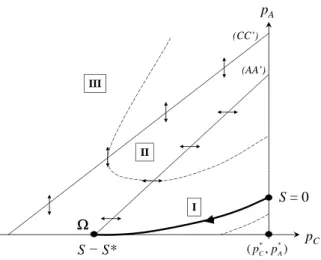
The phase diagram in Figure 1 indicates the shape and relative positions of the trajectories satisfying equations (10) and (11) for a non empty (AA0). We define the lowest region, I, as the triangle having (AA0) as a side and (p∗C, p∗A) as a vertex; the intermediate region, II, lies between the two lines, and the highest region III is above (CC0). In I, p0C < 0 and p0A < 0;
in II, p0C > 0 and p0A> 0; in III, p0C > 0 and p0A> 0.
(CC’) pA III (AA’) II S = 0 I S = S* I pC * * (pC,pA) S S (pC,pA)
Figure 1: Phase diagram.
3.2
Characterization
Proposition 1.
1. There is storage in equilibrium (i.e. S∗ > 0) if and only if
(r + λC)p∗A− λCp∗C + c < 0.
2. The equilibrium trajectory {(pC[S], pA[S]) | S ∈ [0, S∗]} is in region I. It starts with
pC[0] = p∗C and, if S
∗ > 0, it stops at (p
C[S∗], pA[S∗]) = Ω.
4. The equilibrium is unique.
The condition for positive storage has a simple interpretation: crises have to be suffi-ciently likely or suffisuffi-ciently marked to justify storage. Otherwise, there would be no stocks in equilibrium: the price would simply alternate between p∗A in state A and p∗C in state C. To avoid this uninteresting case, we assume in the rest of the paper that the condition for positive storage is satisfied.
The overall behavior of the prices in equilibrium can be summarized as follows: stocks are drained during scarcity episodes and accumulated during abundance episodes.
3.3
Computations
The equilibrium trajectory can be parameterized as pA[pC], a monotone function mapping
[r+λC λC p ∗ A+ c λC, p ∗ C] into [p ∗
A, pA[p∗C]]. Remark that along the equilibrium trajectory pA[pC],
dS dpC
= ∆C[pC]
(r + λA)pC− λApA[pC] + c
, (14)
is well defined over the range of pC, i.e. [r+λλ C
C p
∗
A+λcC, p
∗
C], because the trajectory is bounded
away from (CC0). S∗ can be computed as
S∗ = Z p∗C r+λC λC p ∗ A+ c λC ∆C[pC] (r + λA)pC− λApA[pC] + c dpC. (15)
Numerically, the argument used in the proof of Proposition 1 (point 4) has a very useful implication. In the phase diagram, any point slightly above Ω is on a trajectory that is closer to the equilibrium trajectory as S decreases. In other terms, when we approximate the equilibrium trajectory by another slightly above, the maximum error on price pA[pC] is
at the starting point pC = r+λλ C
C p
∗
A + c
λC. Given that ∆C[·] has a bounded derivative, this
implies that equation (15) can be used to calculate S∗ as accurately as desired by using an approximation of pA[pC].
This allows us to suggest the following algorithm to calculate the equilibrium.
Algorithm 1 (Trajectory and maximum inventories).
1. Fix arbitrarily the upper bound of inventories at some arbitrary value S.
2. Choose ε > 0 as small as needed. Consider the trajectory through (pC[S] = r+λλ C
C p ∗ A+ c λC, pA[S] = p ∗ A+ ε), a point above Ω.
3. Solve the differential equations (10) and (11) numerically and find the stock S(< S) such that pC[S] = p∗C (the trajectory hits the vertical axis and stops). We have the
approximate trajectory.
4. Sε∗ = S − S approximates the upper bound S∗.
5. Shift the calculated functions pC and pA to the left by an amount S to have approximate
equilibrium functions (pC[S], pA[S]) defined over [0, Sε∗].
4
Behavior of the economy
4.1
Comparative statics
In the absence of an explicit expression of price functions and S∗, comparative statics rely
on the properties of the phase diagram.
Proposition 2 (Comparative statics). For all S in the support, and for all states σ = C, A
∂p∗σ[S] ∂c < 0; ∂p∗σ[S] ∂r < 0; ∂p∗σ[S] ∂λA < 0; ∂p ∗ σ[S] ∂λC > 0. (16) and consequently ∂S∗ ∂c < 0; ∂S∗ ∂r < 0; ∂S∗ ∂λA < 0; ∂S ∗ ∂λC > 0. (17)
Interpretations are straightforward. An increase in the unit storage costs discourages accumulation, thus at any level of the stocks, the value of the commodity is smaller. Storers will tend to pile up stocks more slowly in abundance, and to run them down faster during crisis. Similarly, rarer crises diminish the expected yield from storing. This reasoning has direct consequences on the comparative statics of the limit stock: the value S∗, defined as the solution to equation p∗A[S] = p∗A, must decrease if the function p∗A[S] is diminished.
Linear case. The effects of varying excess supply functions are difficult to understand if we do not restrict the analysis to a specific parametric family. For example, in the noteworthy case of linear excess supply functions, analytical results can be found.
Proposition 3 (Linear case). Assume that
∆σ[pσ] = βσ(pσ− p∗σ) with βσ > 0 and p∗σ > 0. (18)
For all S in the support and all states σ = C, A ∂p∗σ[S] ∂p∗C > 0; ∂p∗σ[S] ∂p∗A > 0; ∂p∗σ[S] ∂βC > 0;∂p ∗ σ[S] ∂βA < 0. (19)
and consequently ∂S∗ ∂p∗ C > 0;∂S ∗ ∂βC > 0; ∂S ∗ ∂βA < 0. (20) The sign of ∂S∂p∗∗ A is ambiguous.
A higher price p∗C clearly increases the value of storage, hence the effect on prices and maximum stocks. In contrast, a bigger p∗
A has two effects: on the one hand, it increases
the price at which stocks are built and thus prices in crisis have to increase altogether to motivate positive holding; on the other hand, the range of prices tightens, meaning that potential gains from the occurrence of a crisis could vanish at smaller values of S. This explains the ambiguity of the impact of p∗A on S∗.
A higher parameter βC means that the profitability of storing in view of releasing at high
price when state C arises is better warranted. This gives incentives to store more. A higher parameter βA implies that building stocks is easier, since piling up has a lesser inflationary
effect on the price, hence the negative effect on the equilibrium price.
4.2
Approximate price functions
To better describe the behavior of the economy, we clarify the properties of the equilibrium when stocks are almost empty or close to their maximum. We see in particular how stocks are drained down and why the maximum stocks are not attained in finite time.
Draining out the stock around S = 0. At S = 0, the RHS of equation (10) is non null. We show in Appendix A.4 that
pC[S] − p∗C = − s 2KC ∆0C[p∗C]S 1/2 + o(S1/2) (21)
with KC = (r + λA)p∗C + c − λApA[0] > 0. pC is vertically tangent at 0 (Figure 2). As a
consequence, if the economy stays in crisis, complete drainage of the stocks happens in finite time. To see that, it suffices to integrate in a neighborhood of 0 the differential equation
dSt dt σ t is and stays at C = ∆C[pC[St]], (22)
where the RHS can be replaced by its approximation. As long as the economy stays in crisis, starting with S at date t, the integration of equation (22) yields, for h > 0
S(t + h) = √ S − s ∆0C[p∗C]KC 2 h 2 + o(h). (23)
Drainage exhibits smooth landing: the limit of the withdrawal rate is zero; but drainage time T (S) is finite, that is T (S) = s 2S ∆0C[p∗C]KC + o(√S). (24)
This implies that the economy is protected only about twice as long when stocks are quadru-pled.
The comparative statics on KC is based on (16) in Proposition 2. We have ∂K∂λC
C < 0,
meaning quite naturally, that a larger propensity to return to the scarcity state slows down drainage for precaution motives. Also, ∂KC
∂c > 0 and ∂KC
∂r > 0, meaning that higher storage
costs accelerate drainage for given stocks. Remark that ∂KC
∂λA = (p ∗ C − pA[0]) − λA ∂p∗ A[0] ∂λA > 0 :
a higher propensity to return to abundance also accelerates drainage (preservation value is diminished).
Replenishing. The upper bound S∗ corresponds to singular point Ω. The calculation of an approximate solution requires several steps exposed in Appendix A.4. We get
pA[S] − p∗A = KA(S − S∗) + o(S − S∗), (25)
where KA is a non negative constant calculated in the Appendix. This implies that pA has
a negative finite non-null derivative at S∗ (Figure 2).
Even if the economy stays in a state of abundance, the upper bound S∗is never reached in finite time. The reasoning reminds us of one of Zeno’s classical paradoxes. As pA covers half
itsdifference with the limit p∗A, the variation rate of the stock per unit of time, namely ∆A,
is approximately halved (linear approximation of excess demand at p∗A), meaning that the convergence speed dS/dt is approximately halved. This implies that, whatever the proximity of the target, the duration to cover half the distance to the target is approximately constant, thus the target is never attained.
Example. Using the algorithm of subsection 3.3, we solve numerically the system with the parameters in Table 1. The time unit is the year. We find approximately S∗ ' 9.5. See
Figure 2.
Table 1: Parameter values
Financial and physical costs r = .1 c = .1
Linear excess supply βC = 1 p∗C = 5 βC = 5 p∗A = 1
* C
p
Cp
4
4
C
3
A
A
2
* Ap
Ap
S*
2
4
6
8
Figure 2: Price functions.
5
Stock statistics
A state is described by the stock S and the conjuncture (C or A). We have a unique stationary distribution.11 This section is essentially devoted to the analysis of this stationary
distribution.
5.1
Dynamics
Interior states (i.e. for S ∈ (0, S∗) are just crossed as accumulation or drainage goes on; boundary states, if reached, remain in force until a downward or upward jump occurs. Thus, in the long run, S = 0 and S = S∗ are associated with probabilities whereas values in between are associated with densities.
11Indeed, condition M in Stokey and Lucas (1989, page 348), which is itself a sufficient condition for the
Doeblin condition D page 345, can be employed. The arguments are given for discrete time models, but adapation to our case of continuous time is easy: it suffices to reason with a given finite duration δ and to work with the so-called δ-transition probability derived from following our continuous process for this duration δ. State {C, S = 0} has positive probability whatever the initial state after a certain duration (here after a certain number of iterations of the δ-transition probability). Condition M is trivially satisfied since the state {C, S = 0} is particular: it happens with positive probability (not just density) after some time which is uniformly bounded. Starting from any state, it suffices to have a sufficiently long crisis episode to have depletion; moreover, the economy stays there for a non-negligible duration, since a transition from crisis to abundance may take some time.
Densities. Assume that, for interior values of the stock S ∈ (0, S∗), a density fσ[S, t] (with
σ = C, A) represents the information we have on the system. Take σ = C to fix ideas.
Choose S1 and S2 (0 < S1 < S2 < S∗) two levels of the stocks. By definition
P[C, S ∈ [S1, S2], t] = Z S2 S1 fC[S, t]dS. (26) This gives dP[C, S ∈ [S1, S2], t] dt = fC[S1, t] · ∆C[pC[S1]] − fC[S2, t] · ∆C[pC[S2]] +λC Z S2 S1 fA[S, t]dS − λA Z S2 S1 fC[S, t]dS, (27)
where the first two terms represent the endogenous evolution of the stocks if the economy remains in crisis, and the third and fourth terms represent the exogenous jumps in and out of the segment due to state changes. Figure 3 illustrates this probability balance.
Mass going out Mass coming in
dt S p t S fC[ 1, ]C[ C[ 1]] fC[S2,t]C[pC[S2]]dt
C
C
Jumps Jumps in and outA
A
0
S
S
S*
0
S
1S
2S*
Figure 3: Probability balance between t and t + dt.
To find the dynamics of the density, we make S2 converge toward S1 to get
dfC[S, t] dt = − d dS (fC[S, t] · ∆C[pC[S]]) + λCfA[S, t] − λAfC[S, t]. (28) Similarly dfA[S, t] dt = − d dS(fA[S, t] · ∆A[pA[S]]) + λAfC[S, t] − λCfA[S, t]. (29)
Probabilities. States S = 0 or S∗ are associated with probabilities. We have12
dP[C, 0, t]
dt = −λAP[C, 0, t] − limS→0(fC[S, t] · ∆C[pC[S]]) , (30)
where the first-term represents jumps out (jumps in are negligible since P[A, 0, t] = 0 : due to accumulation, this state is left as soon as attained), and the second term represents the depletion of the last remaining stock.
Similarly, dP[A, S∗, t] dt = −λCP[A, S ∗ , t] + lim S→S∗(fA[S, t] · ∆A[pA[S]]) . (31)
5.2
Stationary distribution
The study of stationary distribution can use directly the preceding analysis. We denote the stationary densities by fσ∗[S] for all S ∈ (0, S∗) and the stationary probability by P∗. Define
φC[S] ≡ fC∗[S] · ∆C[pC[S]] and φA[S] ≡ fA∗[S] · ∆A[pA[S]] (density flows). Dropping the
time-dependency factor, and replacing the rates of variation of the stocks by their equilibrium values, equations (28,29) become the system of ordinary differential equations
dφA dS = λAf ∗ C − λCfA∗, (32) −dφC dS = λAf ∗ C − λCfA∗. (33)
We also have from (30, 31)
P∗[0] = 1 λA lim S→0φC, (34) P∗[S∗] = 1 λC lim S→S∗φA. (35) Remark that −φC[S] = φA[S]. (36)
Indeed, consider the set of states {(C, s), (A, s) | s ∈ [0, S]}, this equation states that, in a stationary distribution, density flows in (at S for state C) equal flows out (at S for state A). Jumps do not matter since they happen within the system.
Equations (32) and (33) collapse to:
dφA dS = − λA ∆C[pC[S]] + λC ∆A[pA[S]] ! φA. (37)
This first order ordinary differential equation is well defined for S ∈ ]0, S∗[ and can be solved numerically. The Cauchy-Lipschitz theorem is applicable.
12This expression can be derived from (27) with S
Algorithm 2 (Stationary distribution).
1. Calculate equilibrium prices pC[S] and pA[S] with Algorithm 1.
2. Fix arbitrarily φA[S] as an initial condition for some S ∈ (0, S∗).
3. Solve numerically the differential equation (37) over ]0, S∗[.
4. Calculate conditional densities fA∗ and fC∗. 5. Calculate the integrals over ]0, S∗[ of fA∗ and fC∗.
6. Use the facts that P∗[S∗] = 0, P∗[S = 0 | C] = 0 and P∗[C] = λA/(λC+ λA) to normalize
fC∗, and then fA∗.
7. Use the facts that P∗[A] = λC/(λC + λA) to calculate the residual P∗[0].
Step 3 must be analyzed in detail. Indeed, ∆C[pC[0]] = ∆C[p∗C] = 0 and ∆A[pA[S∗]] =
∆A[p∗A] = 0, meaning that φA might diverge in such a way that normalization is impossible
(integrals at step 5 could diverge). In fact, we check in Appendix A.5, that
Z S∗ 0 fC∗[S]dS < +∞ and Z S∗ 0 fA∗[S]dS < +∞. (38)
The numerical analysis gives instructive results on the overall behavior of the economy: How frequent are stockouts, i.e. how much is P∗[S = 0] compared to P∗[C] (= λC
λC+λA)? Is the
economy often close to having maximum stocks or is S∗ a practically unapproachable limit? The last question can be addressed theoretically by characterizing the shape of the density of the stationary equilibrium around S∗. Here we can identify which are the critical parameters that determine the regime of the economy.
Figure 4 shows the stationary densities for the parameters in Table 1. We find P∗[0] = .1, P∗[S∗] = 0. In fact limS→0fC = +∞, but fC is approximately proportional to 1/
√
S at
0, meaning that the probability of C remains finite (see equation 34). This high density around 0 comes from the fact that the rate of consumption of the stocks decreases steeply as S approaches zero. The high density on the left of S∗ is explained by the fact that accumulation slows down as the stock approaches S∗(see equations (23,24) about drainage speed and time).
In contrast to 0, S∗ is never attained, as we mentioned in Subsection 4.2. Neverthe-less, as Proposition 4 shows, the probability mass can be quite concentrated, under precise circumstances, in the neighborhood of the maximum.
0.2
0.15
A
0.1
C
A
0.1
0.05
S*
2
4
6
8
Figure 4: Densities. Proposition 4. Let KS∗ = 2 √ 2λC √ ∆0A[p∗A]√(r+λC)2+4∆0A[p ∗ A]λCM −r−λC (39) with M = [(r+λA)(r+λC)−λAλC]p∗A+(r+λA+λC)c −λC∆C[r+λCλC p∗A+ c λC] > 0. (40)At S∗, fC is of the order of (S∗− S)KS∗ and fA is of the order of (S∗− S)KS∗−1.
Consequently,
1. If KS∗ < 1 : fA increases and diverges as S → S∗. Though the maximum is never
attained, any neighborhood of S∗ has a positive probability.
2. If 1 < KS∗ < 2 : fA converges to 0 at S∗ with vertical negative slope. The system is
close to the maximum with a positive probability.
3. If KS∗ > 2 : fA converges to 0 at S∗ with a null slope. The economy is almost surely
far from the upper bound.
Given the discontinuous nature of the comparative statics, singular cases with either
KS∗ = 1 or KS∗ = 2 would require higher order approximations than the one used in
The understanding of the conditions above is relatively complex since all the fundamental parameters play a role. In particular, no simple comparative statics with respect to r or λC
emerge. In contrast, the effects of c, λA are obvious
∂KS∗
∂c < 0;
∂KS∗
∂λA
< 0. (41)
In the linear case, where in particular ∆0
A[p∗A] = βA, we have ∂KS∗ ∂βC > 0;∂KS∗ ∂βA < 0;∂KS∗ ∂p∗C < 0; ∂KS∗ ∂p∗A < 0. (42)
The comparative statics on KS∗, together with the ones on S∗ exposed in the comments
of Proposition 2, outline a notion of flexibility: the higher KS∗, the less flexible the economy
is. Excess supply functions measure the response of prices to given variations in stocks. Small maximum stocks correspond to flexible economies for which large storage would be useless, and accordingly the economy has, statistically, enough time to approach this modest target during abundance period. On the contrary, large maximum stocks mean that the economy will seize (almost) any opportunity to accumulate, which happens in economies where building stocks is a costly process. Accordingly, it is very likely that the random alternation between abundance and scarcity episodes will keep the economy far from the bliss point.
6
Applications and extensions
In this Section, we extend the model by assessing the impact of three kinds of constraints: politically imposed bounds on prices, non-negligible injection and release costs and limited storage capacity.
Analyzing the impact of a constant price on the dynamic system allows a comparison of the results with those proposed by the abundant literature on stabilization. Following on from this, we show that non-negligible injection and release fees can be modelled as parallel shifts in the functions pA[S] and pC[S]. The main results of our analysis are unaffected by
this generalization. Finally, assuming that storage capacity is exogenously constrained, we show that in the accumulation phase, the maximal stock is attained in finite time. Moreover, the price for storage service suddenly jumps above marginal cost when capacity saturates.
6.1
Stabilization, storage and persistent crises
Assume that a central authority imposes a constant price p∗. A price below p∗Awould not be sustainable in the long run (stock will be drained out shortly). A price above p∗C would cause
never ending accumulation, which would be uneconomical. So, the relevant policies consider
p∗A < p∗ < p∗C. Remark that if we preclude rationing, the policy is not strictly applicable since the price must turn to p∗C when stocks are empty in state C. With rationing, the price may remain formally at p∗, but the marginal shadow value of the commodity would be p∗C anyway.
To summarize the effect of the policy, the simplest approach is to search for stationary distribution. We can solve (37), i.e.
dφA dS = − λA ∆C + λC ∆A ! φA for all S > 0, (43) where λA ∆C + λC
∆A here is a constant (with a constant price, ∆C < 0 and ∆A> 0 are constant).
Define p∗ as the solution to the equation λA∆A[p] + λC∆C[p] = 0.
If p∗ < p∗, then λA
∆C +
λC
∆A > 0 ⇔ λA∆A+ λC∆C < 0 : on average, the economy draws on
the stocks. This implies that φA is decreasing and the density is a decreasing exponential:
lower stocks are more likely. The distribution has an unbounded support, empty stocks in crisis is an event of positive probability during which the price is p∗C.
If p∗ > p∗, then λA
∆C +
λC
∆A < 0 ⇔ λA∆A+ λC∆C > 0 : on average, the economy piles
up stocks. This implies that φA is increasing unboundedly with respect to S. Higher stocks
being increasingly likely, normalization is impossible; in other words there is no well defined stationary distribution. Stocks diverge to infinity with probability one and stabilization, in this sense, succeeds.
The case p∗ = p∗ is intriguing. The economy has no tendency to pile up nor to drain out stocks. The limit density is flat, meaning that the behavior of the system in the long run is unpredictable.
Stabilization should not be understood in the narrow sense of averaging the price that would be observed in the absence of storage capabilities. Remark indeed that p∗, which is the critical threshold, could be higher or lower than the average no-storage price λA
λA+λCp ∗ A+ λC λA+λCp ∗
C. This depends on the sensitivity of excess supply functions to price variations.
The conclusion is straightforward: perfect price stabilization can be reached only if the economy is prepared to let stocks go to infinity. The analysis above is easily extended to the case of limited storage capacity. Any upper bound on stocks leaves positive probability on empty stocks. In that case, the probabilities of full storages and stockouts depends on the policy p∗ chosen.
6.2
Injection and release costs
Denote unit injection cost by i and unit release cost by s. Assume that in each state σ = A, C, and for any stocks level S, there are markets for the commodity outside and inside the reservoir, the prices being respectively pσ[S] and pIσ[S]. The (competitive) equilibrium
between outside and inside markets implies that, whenever S > 0,
pA[S] + i = pIA[S] and pC[S] = pIC[S] + s. (44)
The structure of the system of equations is preserved, with pI
σ replacing pσ. No arbitrage conditions read ∆C[pIC + s] · dpI C dS = (r + λA)p I C − λApIA+ c, (45) ∆A[pIA− i] · dpI A dS = (r + λC)p I A− λCpIC+ c. (46)
Remark that the excess supply functions are shifted, thus boundary conditions are
pIC[0] = p∗C − s, (47)
pIA[S∗] = p∗A+ i. (48)
The range of pI
σ is narrower than that of pσ : the minimum is higher, the maximum is lower.
As a result, the condition ensuring that there is storage in equilibrium is more restrictive than the one in Proposition 1 (Point 1), i.e. in the linear case
p∗C − s > r + λ λC ! (p∗A+ i) + c λC . (49)
The phase diagram enables us to show that S∗ is decreasing with respect to the cost param-eters s and i. The rest of the comparative statics is identical.
6.3
Limited storage capacity
If the total storage capacity S exceeds S∗, then the unconstrained trajectory remains sus-tainable; else, rational storers anticipate that boundary conditions are modified.
As long as some capacity is vacant, then storage price per quantity unit (and per unit of time) remains equal to marginal cost c; the system of equations is exactly the same as the one without any constraint, so the equilibrium is described by a trajectory in region I of the phase diagram. Trajectories below the unconstrained equilibrium start on the vertical axis at a given price for S = 0 and stop on the horizontal axis on the right of Ω for a maximum
stock which is smaller than S∗. There is a unique trajectory such that this maximum stock equals exactly S. It describes the unique equilibrium with limited storage capacity. See for example the dashed trajectory below the bold one in Figure 1.
In the accumulation phase, the price for storage service suddenly jumps above marginal cost when capacity is saturated. We denote it by πA.13 Given that pA[S] = p∗A, the
no-arbitrage argument in state (A, S = S) can be expressed
λC(pC[S] − p∗A) = rp
∗
A+ πA. (50)
The LHS measures the potential profit from holding stocks and the RHS the cost. Given that
pC[S] > r+λλCCp∗A+ c
λC (the terminal point is on the right of Ω in Figure 1), we have πA> c.
In contrast to the unconstrained case, the maximal stock is attained in finite time if abundance lasts long enough. This explains that the jump in the price of storage services (a discontinuity) is consistent with a continuous price function pA[S] (continuity is necessary
for no-arbitrage): before the capacity is full, the price pA[S] decrease steadily; storers incur
non-negligible capital losses if the state does not change; this depreciation term does not converge to zero as the maximal stocks are reached; this term is relayed by cost πA> 0 when
the constraint becomes binding.
7
Conclusion
Our model has fully described the behavior of a Markov economy in which storage dynamics are determined by random occurrence of crises. Overall, we have proposed the quite appealing notion of “flexible economy”. We have proved that in equilibrium, a more flexible economy (i.e. better able to absorb shocks via production and consumption changes), is less keen to build up large stocks and is much more likely (in terms of probability) to hold maximum stocks. If the reluctance to build large stocks is intuitive, since overall, the value of stocks (or the convenience yield) decreases when an economy can promptly react to a shock, release dynamics are less intuitive. We show that flexible economies go fast towards maximum stocks and just stay there until a shock leads to fast drainage, while inflexible economies incur permanent movement of their stocks, and over a wider interval. This relationship between flexibility and maximum stocks is a result of interest. On this ground, it could be argued that security of supply policies for energy or banking rules for emission rights, which
13In case of crisis, the stock immediately starts being used so that state (C, S = S) does not last. This
implies that πC, the price of storage services for congestion during the crisis, has no measurable economic
are never neutral with respect to the market equilibrium, should not be set equally across European states, inasmuch as their capabilities to respond to shocks is heterogeneous.
References
[1] Carlson, Dale A; Sholtz, Anne M. (1994): “Designing Pollution Market Instruments: A Case of Uncertainty,” Contemporary Economic Policy, 12, 114-125.
[2] Chambers, Marcus J.; Bailey, Roy E. (1996): “A Theory of Commodity Price Fluctua-tions,” Journal of Political Economy, 104, 924-957.
[3] Chaton, Corinne; Creti, Anna; Villeneuve, Bertrand (2009): “Storage and Security of Supply in the Medium Run,” Resource and Energy Economics, 31, 24-38.
[4] Chevallier, Julien (2012): “Banking and Borrowing in the EU ETS: A Review of nomic Modelling, Current Provisions and Prospects for Future Design,” Journal of Eco-nomic Surveys, 26, 157-176.
[5] Crawford, Vincent; Sobel, Paul Joel; Takahashi, Ichiro (1984): “Bargaining, Strate-gic Reserves, and International Trade in Exhaustible Resources,” American Journal of Agricultural Economics, 66, 472-80.
[6] Deaton, Angus; Laroque, Guy (1992): “On the Behaviour of Commodity Prices,” Review of Economic Studies, 59, 1-23.
[7] Deaton, Angus; Laroque, Guy (1996): “Competitive Storage and Commodity Price Dynamics,” Journal of Political Economy, 104, 896-923.
[8] Devarajan, Shantayanan; Weiner; Robert J. (1989): “Dynamic Policy Coordination: Stockpiling for Energy Security,” Journal of Environmental Economics and Management, 16, 9-22.
[9] Edward, Robert; Hallwood, Charles P. (1980): “The Determination of Optimum Buffer Stock Intervention Rules,” Quarterly Journal of Economics, 94, 156–166.
[10] Ejarque, João Miguel (2011): “Evaluating the economic cost of natural gas strategic storage restrictions,” Energy Economics, 33, 44-55.
[11] European Regulation No 994/2010 concerning measures to safeguard security of gas supply and repealing Council Directive 2004/67/EC.
[12] Helmberger, Peter; Weaver, Rob (1977): “Welfare Implications of Commodity Storage Under Uncertainty,” American Journal of Agricultural Economics, 59, 639–651
[13] Hillman, Arye L.; Van Long, Ngo (1983): “Pricing and Depletion of an Exhaustible Resource when There is Anticipation of Trade Disruption,” Quarterly Journal of Eco-nomics, 98, 215-233.
[14] Hogan, William (1983): “Oil Stockpiling: Help Thy Neighbor,” Energy Journal, 4, 49-71. [15] Hughes Hallett, A.J. (1984): “Optimal Stockpiling in a High-Risk Commodity Market:
The Case of Copper,” Journal of Economic Dynamics and Control, 8, 211-38.
[16] Massel, Benton (1961): “Price Stabilization and Welfare,” Quarterly Journal of Eco-nomics, 83, 284–298.
[17] Montero, Juan P. (1997): “Marketable Pollution Permits with Uncertainty and Trans-actions Costs,” Resource and Energy Economics, 20, 27-50.
[18] Newbery, David; Stiglitz, Joseph E. (1981): The Theory of Commodity Price Stabiliza-tion, Oxford University Press.
[19] Nichols, Albert; Zeckhauser, Richard (1977): “Stockpiling Strategies and Cartel Prices,” Bell Journal of Economics, 8, 66-96.
[20] Oi, Walter (1961): “The Desirability of Price Instability Under Perfect Competition,” Econometrica, 29, 58–64.
[21] Routledge, Bryan R.; Seppi, Duane J.; Spatt, Chester S. (2000): “Equilibrium Forward Curves for Commodities,” Journal of Finance, 55, 1297-1338.
[22] Schennach, Susanne M. (2000): “The Economics of Pollution Permit Banking in the Context of Title IV of the 1990 Clean Air Act Amendments,” Journal of Environmental Economics and Management, 40, 189-210.
[23] Stiglitz, Joseph (1977): “An Economic Analysis of the Conservation of Depletable Nat-ural Resources,” Draft Report, IEA, Section III.
[24] Stokey, Nancy L.; Lucas, Robert E. (1989): Recursive Methods in Economic Dynamics, Harvard University Press.
[25] Sweeney, John (1977): “Economics of Depletable Resources: Market Forces and In-tertemporal Bias,” Review of Economic Studies, 44, 125-142.
[26] Turnovsky Stephen, J. (1974): “Price Expectations and the Welfare Gains from Price Stabilization,” American Journal of Agricultural Economics, 56, 706–716.
[27] Turnovsky Stephen, J. (1976): “The Distribution of Welfare gains from Price Stabi-lization: the case of Multiplicative Disturbances,” International Economic Review, 17, 133–148.
[28] Waugh, Frederic V. (1944): “Does the Consumer Benefit from price Instability?” Quar-terly Journal of Economics, 53, 602–614.
[29] Williams, Jeffrey C.; Wright, Brian D. (1991): “Storage and Commodity Markets,” Cambridge University Press.
A
Appendix
A.1
Proof of Proposition 1
Figure 1 summarizes the shapes and directions of the trajectories.
1. and 2. If (r + λC)p∗A − λCp∗C + c < 0, then S∗ = 0, pC[0] = p∗C and pA[0] = p∗A
cannot be an equilibrium. Indeed, in a competitive economy, a storer who anticipates this dynamics expects other storers not to store, but he sees a profitable opportunity: replenishing at price p∗A when abundance returns is profitable in expectation. Similarly, if the inequality is reversed, no storage is an equilibrium.
All trajectories passing in region II all pass in region III. This is due to the fact that trajectories in region II necessarily go North-West and cross (CC0).
Trajectories in region III, in turn, all go North-East and end up on the vertical axis for finite prices. Indeed, using (10) and (11), we see that p0A/p0C is necessarily bounded above as
pA goes to infinity while pC stays below p∗C (no vertical asymptote). Notice that when the
trajectory crosses {(pA, pC) | pC = p∗C} at time t, the RHS of (10) is strictly positive. This
implies, from equation (4), that pC, as a function of time, will continue to increase, while
inventories stop increasing and start decreasing (p∗C is the zero of ∆C[·]). This contradicts
our assumption that the price only depends on the state. As a consequence, all trajectories passing in II or III are eliminated. This means also that all trajectories starting in I and entering into II can be eliminated, as all of them end in region III.
Trajectories in I that remain candidates all go through {(pA, pC)|pA = p∗A}, somewhere
between Ω and the origin (p∗A, p∗C). All but one cross the horizontal axis, which leads to the same type of contradiction as in the previous paragraph between seeing the price as a function of time and as a function of. We eliminatetrajectories that do not reach Ω. Recall that Ω is a stopping point both with respect to time (the RHS of (5) is null) and inventories (pA= p∗A).
3. Remark that |dpC/dS| is bounded away from 0 along the trajectory. The range of pC[·]
being bounded, S can only vary in a bounded interval. Therefore S∗ is finite.
4. We now show that the trajectory passing through Ω is unique. The Cauchy-Lipschitz Theorem cannot be applied at Ω, a singular point of the system. We use the following ar-gument: choose any starting point in the interior of I, denoted by (p0C, p0A); it is necessarily nonsingular. The trajectory passing through this point is unique (Cauchy-Lipschitz). Con-sider the point (p0
C, p0A+ ε) where ε is some small real. Straightforward calculations show
that the slope of the trajectory passing through (p0
C, p0A+ ε), which is positive, decreases as
ε increases. To see this, one can directly reason on dpA/dpC = ∆C[pC] ∆A[pA] · (r + λC)pA− λCpC + c (r + λA)pC− λApA+ c . (51)
This means that trajectories move apart as S increases, i.e. as they approach Ω. The conse-quence is that there cannot be multiple trajectories through Ω. This proves uniqueness.
A.2
Proof of Proposition 2
We first determine how trajectories move in the phase diagram as parameters change. Rewrite the system of ODE (10) et (11) in compact form as
p0C = PC(pC, pA, c, r, λA, λC) or simply PC ( > 0 in region I), (52)
p0A = PA(pC, pA, c, r, λA, λC) or simply PA ( < 0 in region I). (53)
Note that ∂PC ∂c = 1/∆C[pC] < 0 and ∂PA ∂c = 1/∆A[pA] > 0, thus p 0 A/p 0 C = PA/PC decreases as
c increases (all trajectories in I are flatter). Similar observations prove that all trajectories
in I are also flatter when r increases, when λA increases and when λC decreases.
We can now reposition equilibrium trajectories as parameters change. Increasing c or r, or decreasing λC, move Ω to the right; increasing λA has not effect on Ω. In all cases, the
Remark that dpdS C = 1/PC < 0, thus S = − Z p∗ C pC[S] dpC PC
(summation along the equilibrium trajectory). (54) Since Ω goes to the right as c increases, the range of pC becomes smaller; it remains to be
verified that 1/PC, as a function of pC, is also smaller. For example, along the equilibrium
trajectories, for a fixed pC
dPC dc = 1 ∆C[pC] | {z } − +∂pA ∂c | {z } − ×∂PC ∂pA | {z } + < 0. (55)
(PC grows in absolute value and thus 1/PC decreases in absolute value.) This proves that as
c increases, a given price is associated with a smaller S. Similar reasonings can be applied
to the other parameters to prove the claims.
A.3
Proof of Proposition 3
We have PC = (r + λA)pC− λApA+ c βC(pC − p∗C) , (56) PA = (r + λC)pA− λCpC + c βA(pA− p∗A) . (57)
Clearly, trajectories in I are steeper with a higher βC or a smaller βA. Remark that the
frontier of I (Ω in particular) is unchanged in this comparative statics. Remark also (this concerns point 2) that a proportional increase of βC and βA does not change the trajectories
(but a given point corresponds to a different S). The type of reasoning used in the proof of Proposition 2 can now be applied to show the claims.
The comparative statics with respect to p∗C and p∗A require further precautions. In the former, remark that trajectories are steeper with a higher p∗
C (pC < p∗C) and that I is extended
to the right (trajectories are simply going further to the right). These two effects concur to increase the price for given stocks. In the latter, trajectories are flatter with a (say) smaller
p∗A but Ω moves along down (AA0). The first effect decreases prices, hence point 1, but the second could lead to a higher S∗ (a smaller function is integrated over a longer interval, since the range of pC increases, see equation 54).
A.4
Equivalent expressions for prices
On the right of S = 0. From (10), we know that
thus, writing approximations on both sides we get 1 2∆ 0 C[p ∗ C](pC[S] − p∗C)2+ o(pC[S] − p∗C)2 = KCS + o(S), (59)
which yields equation (21).
On the left of S = S∗. Let x0A denote ∆A[pA] · p0A. Given that p
0
C[S
∗] 6= 0, we can
approximate pC[S] around S∗ with pC[S∗] + p0C[S
∗](S − S∗) + o(S − S∗). We denote −p0
C[S
∗]
(which can be calculated exactly using (10)) by M , with
M = −[(r+λA)(r+λC)−λAλC]p∗A+(r+λA+λC)c λC∆C[r+λCλC p∗A+λCc ] > 0. (60) Given that xA[S] = Z p∗A pA[S] ∆A[p]dp, (61)
we can calculate that pA[S]−p∗A+o(pA[S]−p∗A) =
q 2 ∆0A[p∗A]x 1/2 A [S], or equivalently pA[S]−p∗A= q 2 ∆0A[p∗A]x 1/2 A [S] + o(x 1/2
A [S]). We plug these two equivalent expressions into (11), which yields
x0A= v u u t 2(r + λC)2 ∆0 A[p∗A] x1/2A + λCM (S − S∗) + o(S − S∗) + o(x 1/2 A ), (62)
Consider now the ODE
y0 = v u u t 2(r + λC)2 ∆0A[p∗A] y 1/2 + λCM (S − S∗) with y[S∗] = 0. (63)
The unique solution to (63) is K2
A(S ∗− S)2 with KA= √ (r+λC)2+4∆0A[p∗A]λCM −r−λC 2√2∆0A[p∗A] . (64)
We show now that this exact solution of approximate ODE (63) is an approximation of the solution to ODE (62).
Consider the residual o(S − S∗) + o(x1/2A [S]) in the ODE (62). For all ε > 0, there is a left neighborhood of S∗, denoted V
ε, in which the absolute value of the residual is smaller than
ε × (S∗− S) and ε × (x1/2A [S]). Consider the ODE
y0 = v u u t 2(r + λC)2 ∆0 A[p∗A] + ε y1/2+ (λCM − ε)(S − S ∗ ) with y[S∗] = 0. (65)
The solution to this equation is smaller than xAon Vε: indeed, both x0A and y0 are negative,
but if y > xA for some S in Vε, it remains so for any larger stock because y0 > x0A. This is in
contradiction with the fact that y[S∗] = xA[S∗]. In other terms,
xA[S] ≥ r (r+λC+ q ∆0 A[p∗A] 2 ε)2+4∆ 0 A[p ∗ A](λCM −ε)−r−λC− q ∆0 A[p∗A] 2 ε 2√2∆0A[p∗A] 2 (S∗− S)2. (66)
A similar reasoning shows that
xA[S] ≤ r (r+λC− q ∆0 A[p∗A] 2 ε)2+4∆ 0 A[p ∗ A](λCM +ε)−r−λC+ q ∆0 A[p∗A] 2 ε 2√2∆0A[p∗A] 2 (S∗− S)2. (67)
These two inequalities give the approximation of xA at S∗, from which we derive that of pA
since pA[S] − p∗A= q 2 ∆0A[p∗A]x 1/2 A [S] + o(x 1/2 A [S]).
A.5
Proof of convergence of Algorithm 2
Remark that the ODE commanding φA can be written
φ0A φA = − λA ∆C + λC ∆A ! . (68)
On the right of S = 0, ∆C → 0 so the RHS of (68) is equivalent to −∆λAC, i.e., using (21), to K0
√
S where K0 is a nonnegative real
K0 =
λA
∆0C[p∗C]√KC
. (69)
Thus limS→0φA is finite and strictly positive. Indeed, for all ε > 0, there exists η such that
for all S ≤ η, (1 − ε)√K0 S ≤ φ0A φA ≤ (1 + ε)√K0 S. (70)
Take S1 and S2 both smaller than η with S1 ≤ S2 and integrate the inequality above between
these two reals. We find 2(1 − ε)K0( q S2− q S1) ≤ ln φA[S2] φA[S1] ≤ 2(1 + ε)K0( q S2− q S1). (71)
This proves that φA is bounded away from 0 (fix S2 and let S1 converge to 0). Given that
φA is also monotonic (increasing) in a neighborhood of 0, the limit that we denote by φA[0]
exists and is nonnegative.
So, at 0, fA is finite and nonnegative whereas fC ∼0
KfC
√
S where KfC is some nonnegative