An extension of analytical methods for building damage evaluation in subsidence regions to anisotropic beams

An extension of analytical methods for building damage evaluation in

subsidence regions to anisotropic beams

SAEIDI Ali

_{, DECK Olivier}

_{, VERDEL Thierry}

a* _{Centre d’études sur les ressources minérales, Université du Québec à Chicoutimi,}

Chicoutimi, Québec, Canada, ali_saeidi@uqac.ca

b _{Université de Lorraine, GeoRessources, UMR 7359, Nancy, F-54042, France,}

An extension of analytical methods for building damage evaluation in

subsidence regions to anisotropic beams

Abstract

Ore and mineral extraction by underground mining often causes ground subsidence phenomena, and may induce severe damage to buildings. Analytical methods based on the Timoshenko beam theory is widely used to assess building damage in subsidence regions. These methods are used to develop abacus that allow the damage assessment in relation to the ground curvature and the horizontal ground strain transmitted to the building. These abacuses are actually developed for building with equivalent length and height and they suppose that buildings can be modelled by a beam with isotropic properties while many authors suggest that anisotropic properties should be more representative. This paper gives an extension of analytical methods to transversely anisotropic beams. Results are first validated with finite elements methods models. Then 72 abacuses are developed for a large set of geometries and mechanical properties.

Type or paste your abstract here as prescribed by the journal’s instructions for authors. Type or paste your abstract here as prescribed by the journal’s instructions for authors. Type or paste your abstract here as prescribed by the journal’s instructions for authors. Type or paste your abstract here.

Keywords: mining subsidence, damage, horizontal strain, curvature, beam theory, anisotropic

Introduction

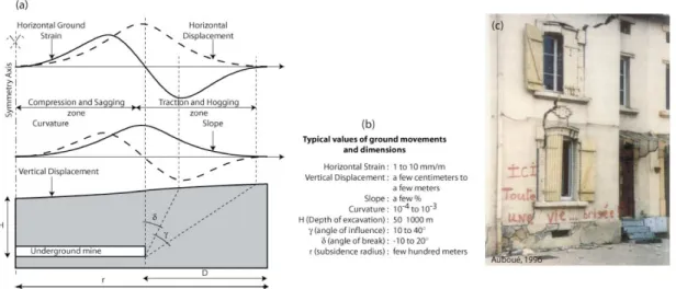
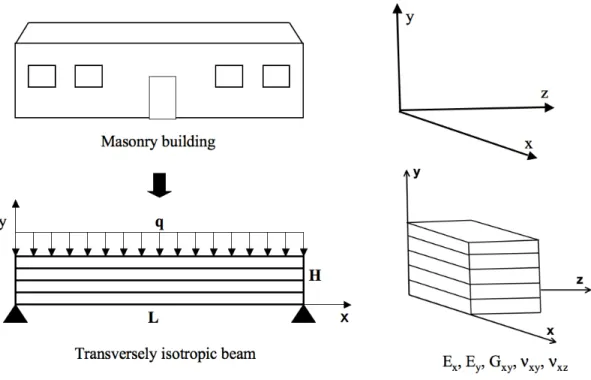
Ore and mineral extraction via underground mining may induce ground subsidence phenomena. These phenomena lead to horizontal and vertical ground movements, which consequently lead to deformations and damage in buildings of undermined urban regions (Figure 1). The maximum vertical displacement occurs in the centre of the subsidence area and may reach several meters. This displacement is accompanied by horizontal ground strains, ground curvature, and slope, the three types of movements that load structures and

cause structural damage (Saeidi, Deck and Verdel, 2013). According to the mining extraction method: longwall mining, rooms and pillars with or without caving… subsidence is planned or may be accidental a long time after the extraction. In all cases, prediction of building damage is necessary when subsidence is expected in an urbanized area.

Dimensions of mining subsidence are basically greater than the buildings ones and the grounds movements may be assumed constant over the building length. Figure 1 described the main dimensions and characteristics of a mining subsidence for a longwall mine. But, at the scale of one building compared to the extension of a mine, these ground movements are quite similar in the case of a subsidence over a rooms and pillars mine with or without caving. Depending to the subsidence kinetic, location of buildings in a subsidence is time dependent. A building may be in the traction and hogging area when the subsidence starts and be in the compression and sagging area when the subsidence stops. When mining subsidence is accidental, the kinetic is generally uncertain and the final location of the building is considered to assess the lower bound of the ground movements in the building vicinity. Two parameters are used to quantify the subsidence intensity in relation to the building damage: the horizontal ground strain that is associated with the horizontal load of the buildings, and the ground curvature that is associated with the deflection of the buildings.

Figure 1. Description of the main characteristics involved in mining subsidence and associated consequences (Saeidi, Deck and Verdel, 2009). a) typical profiles of the ground displacements and localisations of the compression/sagging and the traction/hogging areas. b) Typical values of the subsidence dimension and grounds movements. c) typical damage due to mining subsidence in the city of Auboué, France.

The assessment of building damage in mining subsidence hazard areas can be performed using three types of methods: empirical, analytical and numerical methods. Empirical methods are based on the analysis of a large number of observations of damage to buildings. The simplest method is threshold values of the ground displacements (Skempton and MacDonald, 1956). The National Coal Board method (NCB, 1975) is one of the most famous, and it addresses the damage assessment with the building length and the horizontal ground strain. Analytical methods are based on the use of beam theory (Timoshenko, 1957) to assess the global behaviour of a building in relation to its geometry and mechanical properties. The first method was developed by Burland and Wroth (1974), and many extensions are now available (Boone, 1996; Finno, Voss, Rossow and Blackburn, 2005). Numerical methods are mostly used for the prediction of ground movements (Melis, Medina and Rodríguez, 2002 and Coulthard and Dutton 1998), the study of soil structure

interaction and the assessment of the transmitted ground movements (Selby, 1999, Franzius, Potts and Burland 2006, Son and Cording 2005 and Burd, 2000). But very few studies address the question of the damage assessment with numerical methods.

The analytical methods initially developed by Burland and Wroth (1974) is widely used. This method was used to develop an abacus to assess the building damage, in relation to the horizontal ground strain and the ground curvature transmitted to the building, for a specific configuration: a building with a length L by height H ratio equal to 1 (L/H=1) and isotropic mechanical parameters with E/G = 2.4, with E and G the Young and shear modulus. However, the use of the beam theory for L/H ratio less than two is mostly questionable and such analytical methods should be restricted to greater L/H ratio. Moreover, Son and Cording (2007) show that masonry buildings with openings, required to be modelled with E/G greater than 3, i.e. with a Poisson ratio ν greater than 0.5 is isotropic behaviour is considered. This requires considering anisotropic behaviour.

In the following the analytical method of Burland and Wroth (1974) is first described and extend to transversely anisotropic materials. Results of the improved method are compared with those of finite element methods analysis (CESAR-LCPC, 2010). Then the method is used to plot a set of abacuses in order to cover a large set of dimensions (L/H ratio) and mechanical properties.

Analytical methods for building damage evaluation

Overview

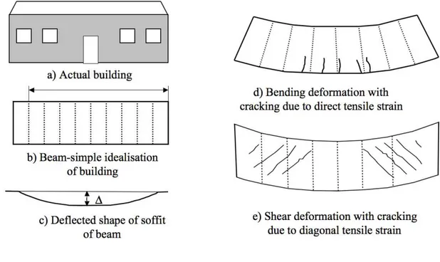
Wroth (1974), and several extensions are now available (Boscardin and Cording, 1989, Boone, 1996 Burland, 1995, Boone, 2001, Finno, Voss, Rossow and Blackburn, 2005). In these methods, masonry buildings are modelled with an isotropic and elastic beam with two supports, loaded by a central or uniformly distributed load. A deflection ∆ is imposed on the beam to model the ground curvature that corresponds to the bending effect of the subsidence on the building (Figure 2). The maximum tensile strains due to bending deformation and shear deformation are then calculated and compared with the values of the critical tensile strains for the determination of the damage class. All of the current analytical methods use five damage classes, and Table 1 gives the five damage classes defined by Burland (1995) and Boscardin and Cording (1989).

Figure 2. Beam model for building in subsidence zone (after Burland, Mair and Standing 2004).

Differences between these methods concern the modelling of the subsidence effect, the loading distribution (building weight), the location of the neutral axis, the building type and

the imposed relationships between the mechanical parameters:

(i) Most of the methods consider the deflection ∆ to model the effect of the subsidence. Boscardin and Cording (1989) extended the approach of Burland and Wroth (1974) by superimposing the horizontal strain εh induced by the horizontal ground strain onto those generated by the bending of the beam. These methods assume that the deflected beam is then also subjected to a uniform extension over its full depth.

(ii) Analytical methods consider different types of buildings. Burland and Wroth (1974), as well as Boscardin and Cording (1989), consider masonry buildings modelled with isotropic beams, and they suggest adjusting the ratio E/G of the Young’s modulus E to the shear modulus G of the beam to be between 2.4 and 12.5, in order to take into account the influence of the openings (doors and windows) that would cause an increase in the shear deformation. Son and Cording (2007) investigated the possible range of the E/G ratio in relation to the number of windows, and they show that this ratio may be close to 60. These values denote an anisotropic behaviour of buildings that is incompatible with the first assumption of an isotropic beam that imposes a E/G ratio between 2 and 3 in order to keep the Poisson ration between 0 and 0.5. Boone (1996, 2001) considers three types of buildings: load bearing wall masonry buildings, in-fill walls and beam-in-frame structures. Finno, Voss, Rossow and Blackburn, (2005) suggest a model to take into account the positive influence of the concrete floors of buildings under study.

(iii) Burland (1995) considered both a uniformly distributed and a central point load to model the building weight. Boscardin and Cording (1989) and Finno, Voss, Rossow and Blackburn, (2005) also considered the central load assumption, while Boone (1996, 2001)

considered the uniformly distributed load assumption. In the present paper, we have selected a uniformly distributed load because it appears to be more realistic than the central point load assumption.

(iv) The localisation of the neutral axis is also a debatable question. In the hogging area, Burland and Wroth (1974) and Boscardin and Cording (1989) consider that the neutral axis is probably located at the bottom of the beam because of the small tensile resistance of the upper levels of the masonry building and the greater tensile resistance of the foundation level. Boone (1996) considers this to be debatable because of the influence of the floors and the roof that may increase the tensile resistance. In our case, we have assumed that the neutral axis is located in the middle, i.e., superimposed on the central axis.

Burland method

As it was explained in the previous section Burland’s method consider the building as an isotropic beam with dimension L for the length, H for the height and with a unit thickness. The beam can be affected both by the horizontal ground strain and the ground curvature. A vertical transmitted deflection ∆ is imposed at the centre of the beam to model the effect of the ground curvature, and a uniform horizontal transmitted strain εh is imposed to model the effect of the horizontal ground strain.

Based on the theory of Timoshenko (1957), Burland and Wroth (1974) identified two critical sections in the beam where maximal tensile strains occur; the half span section and the edge section. In these two sections, the maximal tensile strain must be calculated in order to allow a comparison to threshold values associated with different damage classes.

The relationships between ∆ and the maximum tensile strain εb in the half-span critical section, or the maximal diagonal tensile strain εd in the edge section, are calculated by Burland (1995) according to Equation (1) and Equation (2), where y is the distance between the neutral axis and the lower fibre of the beam.

∆ L = 5⋅L 48⋅y+ 3⋅I 2⋅y⋅L⋅H ⋅ E G      

ε

ε

The effect of the uniform horizontal transmitted strain εh, may then be added in order to calculate the maximal value of the principal tensile strain in the two critical sections.

In the half span critical section, both ∆ and εh induce principal horizontal tensile strains. The maximal tensile strain εbmax is then estimated as the sum of these two principal tensile strains (Equation (3)):

ε

=

ε

+

ε

In the edge critical section, ∆ induces vertical shear stresses and ultimately a diagonal principal tensile strain, while εh induces a horizontal principal tensile strain. The maximal tensile strain εdmax is then evaluated using Mohr’s circle of strain (Equation (4), Burland, Mair and Standing, 2004).

ε

ε

ν

ε

ν

ε

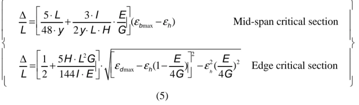
By substituting the values of εb in Equation (1) into Equation (3) and εd in Equation (2) into Equation (4), the relationship between the relative deflection parameter (∆/L), the transmitted horizontal strain (εh) and other building parameters is calculated for the two critical sections (Equation (5)).

∆ L= 5⋅L 48⋅y+ 3⋅I 2y⋅L⋅H⋅ E G     

(

ε

ε

ε

ε

ε

Edge critical section

                  (5)

Burland, Broms and De Mello (1977) defined the concept of limiting tensile strain εlim that must be compared to the maximal tensile strains εbmax and εdmax to define the threshold value of the maximal tensile strain before damage occurs. Like Boscardin and Cording (1989), Burland (1995) defined different threshold values for different damage levels according to Table 1, and they considered these values for a large quantity of buildings. Most of the analytical methods use these thresholds values to assess the building damage, and we have also used the same values.

Table 1. Threshold values of the limiting tensile strain εlim associated with the five damage classes (Boscardin and Cording 1989, Burland, Mair and Standing 2004).

Damage class Limiting tensile stain (εlim)%

D0 Negligible 0-0.05

D1 Very slight 0.05-0.075

D2 Slight 0.075-0.15

D4 and D5 Severe to Very Severe >0.3

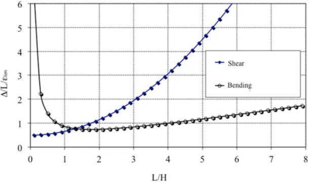
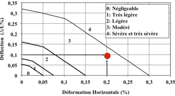
The two relations from Equation (5) are usually used to plot the ∆/(L.εlim) ratio versus the L/H ratio for given values of the building mechanical properties and the uniform horizontal transmitted strain εh. Figure 3 shows a result for the case where εh is set equal to 0, the E/G ratio is 2.6 (case of an isotropic beam with ν = 0.3) and the neutral axis is in the middle. This figure shows two curves: one is associated with the tensile strain due to shear near the edges of the beam (Figure 2-d), and the other is associated with the tensile strain due to bending in the middle span of the building (Figure 2-e). The minimum value of ∆/L/εlim between these two curves is a critical value, and it can be used to assess the maximal admissible relative deflection ∆/L. For a given value of the limiting tensile strain (εlim), the smallest value of ∆/L/εlim between the two curves indicates whether the failure will occur near the edge section (shear) or near the middle section (bending). It appears that for small values of the ratio L/H, failure will occur near the edge of the building where the maximal tensile strain due to shear first reaches the limiting value εlim. For greater values of the ratio L/H, failure will occur in the middle section (Figure 3).

Figure 3. Limiting relationships between (∆/L)/εlim and L/H.

Comparison of Figure 3 and Table 1 is required to plot abacuses of damage in relation to the deflection ratio and the horizontal strain. Burland developed such abacus for a specific situation: a central point load beam model, with L/H=1 and isotropic properties with E/G = 2.6 (ν = 0.3) (Figure 4). The first criticism is that this abacus is developed for a building dimension which doesn’t allow the use of the beam theory. The second is that there is a risk this abacus be used for other shape and mechanical properties, when results may significantly differ.

Figure 4. Burland curve for damage assessment in subsidence zone.

Development of abacuses for isotropic transversally beams.

Burland’s method is based on the Timoshenko beam theory that suppose isotropic materials i.e E/G is between 0.5 and 3 for a Poisson ratio between 0 and 0.5. However several authors suggest to consider greater values of E/G, up to 60 (Boscardin and Cording 1989, Son and Cording 2005, 2007) These values are contradictory with the isotopic assumption and the use of Timoshenko beam theory. Therefore to justify the use of such values in the Burland analytical method, the building is modelled as an elastic and transversely isotropic beam with two supports.

The transversely isotropic behaviour is defined with 5 independents parameters. Two Young’s modulus Ex and Ey, two Poisson’s ratio νxy and νxz and one shear modulus Gxy (Figure 5). Assumptions are made to reduce to 3 the number of independent parameters: Ex

Figure 5. Transversely isotropic beam model for masonry building.

Results of the transversely isotropic beams are similar to Equation (5) before replacing ν by the value E/2G-1 (Equation (6)). Detailed formulas are shown in appendix.

∆ L = 5⋅L 48⋅y+ 3⋅I 2y⋅L⋅H⋅ E G_xy       

(εbmax−εh) M id-span critical section

∆ L= 1 2+ 5H⋅L2G_xy 144I⋅E      ⋅ εdmax−εh( 1−υ 2 )     2 −εh 2₍1+υ 2 )

2 _{Edge critical section}                   (6)

Thus, no difference exists between the isotropic and the transversely isotropic models. Introduction of non-isotropic values of ν and E/G in Burland’s expressions can appear as an heuristic approach to take into account the real anisotropic behaviour of masonry walls. However, Equation (1) and Equation (2) remain similar for isotropic and transversely isotropic models if it is assumed that, the normal to centroidal axis remains normal and straight after bending.

However, it is not at all obvious that this assumption is correct. To validate it, numerical simulations (FEM) are performed.

Validation of the assumption that normal to centroidal axis remains normal and straight after bending

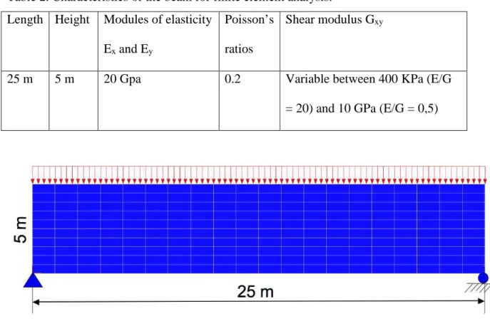
We consider a FEM to model an transversely isotropic (CESAR-LCPC software 2010). Geometry of the model is shown in Figure 6 and the characteristics of the beam are presented in Table 2.

Table 2. Characteristics of the beam for finite element analysis. Length Height Modules of elasticity

Ex and Ey

Poisson’s ratios

Shear modulus Gxy

25 m 5 m 20 Gpa 0.2 Variable between 400 KPa (E/G = 20) and 10 GPa (E/G = 0,5)

Figure 6. FEM model of beam

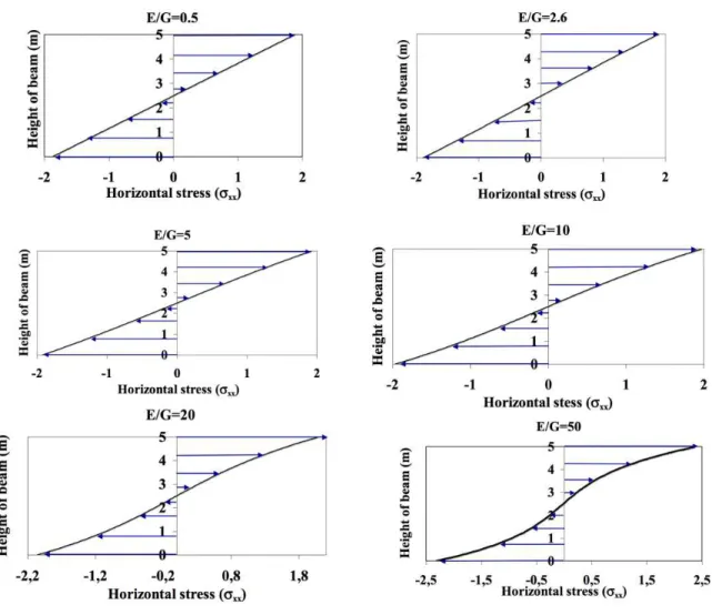
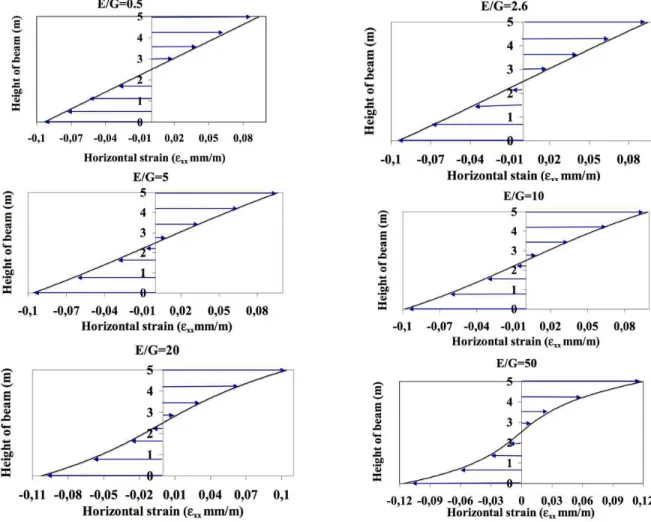
Several values of E/G are considered in the analysis (0.5, 2.6, 5, 10, 15, 20, 50). Figure 7 and Figure 8 show results of σxx stresses and εxx strains in a vertical section at the mid span

of the beam. Results show a linear variation of horizontal stresses for value of E/G less than 50. This confirms the assumption that the normal to centroidal axis remains normal and straight after bending for anisotropic beam (Hashin 1967).

Figure 8. Distribution of εxx on mid-span cross section of the beam (in mm/m).

Moreover, comparison of the maximum deflection calculated with the Timoshenko formulas and transversely anisotropic behaviour (Equation (1) and Equation (4)) and with the FEM shows a good agreement for values E/G less than 50. Consequently, Equation (6) is validated to model transversely isotropic beams.

Figure 9. Comparison of the maximum deflection calculated with Equation (6) and the FEM for transversely isotropic beams.

Application of the transversely isotropic model to develop abacuses

Objective of this section is to develop different abacuses to investigate others cases than the one of Burland (1995). The uniformly distributed load assumption is chosen because it appears more realistic to model the building weight and the neutral axe is taken in the middle of the beam. Different geometries are investigated with L/H ratio between 1 and 4. Opinion of authors is that results for L/H equal to unit are probably not realistic. However these results are useful to be compared with the initial abacus of Burland who used the same geometry. The transversely isotropic model is used so that different values can be investigated both for ν and E/G. The Poisson’s ratio is taken between 0 and 0.5. The E/G ratio is taken between 0.5 and 12.5.

Abacuses are developed with an algorithm presented in the Figure 10.

The first step of the algorithm is to choose a threshold value of critical strain εcr for εbmax

and εdmax, according to Table 1. Then for each value of the horizontal strain transmitted by

the ground to the building εh, we can calculate the value of the ratio ∆/L that satisfies the

equilibrium relationships of the beam (Equation (6)). Two values of ∆/L are obtained when considering the influence of shear or bending moment. Only the minimum value is taken.

By repeating the procedure for all values of the horizontal strain εh, we can draw the

boundary curve of this type of damage. The change εcr value (Table 1.) is then used to draw

Figure 10. Algorithm of determination of damage curve development

Results are all plotted in Figure 11 for L/H =1, Figure 12 for L/H = 2, Figure 13 for L/H = 3 and Figure 14 for L/H = 4. In each figures, 24 abacuses are drawn for each combination of υ and E/G. Several abacuses show broken lines This means that failure may occur both because of bending (right part of the lines) or shear (left part). When abacuses only show straight lines, these correspond to a bending failure. Thus long buildings and buildings with small E/G ratio are most affected by bending, rather than shear.

Abacus in Figure 11, plotted for ν = 0.3 and E/G = 2.6 can be compared with the previous one developed by Burland (Figure 4). Results show that Burland’s assumption: central point load and neutral axis at the bottom of the beam, are not conservative since damage is underestimated with Figure 4 compared with Figure 11.

Results also show a significant influence of the E/G and L/H ratio, while ν is less influent. On the whole, greatest values of E/G and L/H gives smaller damages. However, detailed results show that complex interactions must be considered. This can also be explained with Equation (6), where it is obvious that L/H and E/G have an opposite effect when considering the second equation (shear), while both L/H and H/L appear in the first equation (bending).

All these comparisons demonstrate that none of these damage curves are suitable for all buildings, and that it is important to calculate and use the correct damage curve associated with the most realistic building parameters.

Figure 11. Damage identification curves for buildings for building with L/H ratio ratio equal 1 and different mechanical parameters

Figure 12. Damage identification curves for buildings for building with L/H ratio equal 2 and different mechanical parameters

Figure 13. Damage identification curves for buildings for building with L/H ratio equal 3 and different mechanical parameters

Figure 14. Damage identification curves for buildings for building with L/H ratio equal 4 and different mechanical parameters

Conclusion

Analytical methods based on the Timoshenko beam theory are widely developed to assess building damage in subsidence regions. These methods are developed for isotropic materials and are developed only for a specifically geometry of building especially in the case of building with equivalent length and height. In this paper, a transversely isotropic beam model is investigated and an algorithm is developed to adapt results to a various

dimension and mechanical properties.

Theoretical developments show that the initial formulas of Burland (1995) may be use for anisotropic beams. The use of a transversely isotropic model is adapted for studying masonry buildings whose E/G ratio is shown to reach important values.

References

Boone, S. (1996). Ground-Movement-Related Building Damage. Journal of Geotechnical

Engineering, 122(11), 886-896. doi:

doi:10.1061/(ASCE)0733-9410(1996)122:11(886)

Boone S.J. (2001). Assessing construction and settlement-induced building damage: a return to fundamental principles, Proc. underground construction, institution of

mining and metallurgy, London, 559-570.

Boscardin, M., & Cording, E. (1989). Building Response to Excavation‐Induced Settlement. Journal of Geotechnical Engineering, 115(1), 1-21. doi: doi:10.1061/(ASCE)0733-9410(1989)115:1(1)

Burd, H. J., Houlsby, G. T., Augarde, C. E., & Liu, G. (2000). Modelling tunnelling-induced settlement of masonry buildings. Proceedings of the ICE - Geotechnical

Engineering, 143, 17-29.

Burland J B., & Wroth C P. (1974). Settlement of buildings and associated damage. Conf.

settlement of structures, 611-654.

Burland J B., Broms B B. & De Mello V F B. (1977). Behaviour of foundations and structures. 9th Int.conf. on soil mechanics and foundations engineering, Tokyo 2, 495-546.

Burland J B. (1995). Assessment of risk of damage to building due to tunnelling and

excavation. Proc. 1st Int. Conf. Earthquake Geotechnical Engineering, Ishihara(ed.),

Balkema, 1189-1201.

Burland J B., Mair R J and Standing J R. (2004). Ground performance and building response due to tunnelling. Advance in geotechnical engineering, the skempton

Coulthard M A, Dutton A J. (1998). Numerical modelling of subsidence induced by underground coal mining. The 29th U.S. Symposium on Rock Mechanics (USRMS), Minneapolis, MN.

CESAR-LCPC 2D & 3D finite element package dedicated to solve Civil Engineering problems, École Nationale des Ponts et Chaussées, Paris,2010.

Franzius, J. N., Potts, D. M., & Burland, J. B. (2006). The response of surface structures to tunnel construction. Proceedings of the ICE - Geotechnical Engineering, 159, 3-17. Finno, R., Voss, F., Rossow, E., & Blackburn, J. (2005). Evaluating Damage Potential in

Buildings Affected by Excavations. Journal of Geotechnical and Geoenvironmental

Engineering, 131(10), 1199-1210. doi:

doi:10.1061/(ASCE)1090-0241(2005)131:10(1199)

Hashin, Zvi. (1967). Plane Anisotropic Beams. Journal of Applied Mechanics, 34(2), 257-262. doi: 10.1115/1.3607676

Melis, Manuel, Medina, Luis, & Rodríguez, José Ma. (2002). Prediction and analysis of subsidence induced by shield tunnelling in the Madrid Metro extension. Canadian

Geotechnical Journal, 39(6), 1273-1287. doi: doi:10.1139/t02-073

National Coal Board. (1975). Subsidence engineering handbook. chapter 6, 45-56.

Saeidi, Ali, Deck, Olivier, & Verdel, Tierry. (2009). Development of building vulnerability functions in subsidence regions from empirical methods. Engineering Structures,

31(10), 2275-2286. doi: http://dx.doi.org/10.1016/j.engstruct.2009.04.010

Saeidi, Ali, Deck, Olivier, & Verdel, Thierry. (2013). Comparison of Building Damage Assessment Methods for Risk Analysis in Mining Subsidence Regions.

Geotechnical and Geological Engineering, 31(4), 1073-1088. doi:

10.1007/s10706-013-9633-7

Selby, A. R. (1999). Tunnelling in soils – ground movements, and damage to buildings in Workington, UK. Geotechnical & Geological Engineering, 17(3-4), 351-371. doi: 10.1023/A:1008985814841

Skempton A W., MacDonald D H. (1956). Allowable settlement of building. Proc. INSTN.

Son, M., & Cording, E. (2005). Estimation of Building Damage Due to Excavation-Induced Ground Movements. Journal of Geotechnical and Geoenvironmental Engineering,

131(2), 162-177. doi: doi:10.1061/(ASCE)1090-0241(2005)131:2(162)

Son, M., & Cording, E. (2007). Evaluation of Building Stiffness for Building Response Analysis to Excavation-Induced Ground Movements. Journal of Geotechnical and

Geoenvironmental Engineering, 133(8), 995-1002. doi:

doi:10.1061/(ASCE)1090-0241(2007)133:8(995)

Timoshenko S. (1957). Strength of material-part I, D van Nostrand Co, Inc. London. Wolfram S. (2007). Mathematica software version 6. Wolfram Research, Inc., USA. Deck O. (2002). Study of the effects of mining Subsidence on the structures, Phd thesis,

Appendix 1 : Calculation of the deflection for transversely isotropic beam

In this section, we consider assumption that any cross section, normal to centroidal axis, remains normal and straight after bending, as for isotropic beams. This assumption is necessary to calculate the influence of the bending moment on the deflection, but is not necessary to calculate the influence of the shear force on the deflection. Consequently, the differential equation of the deflection is the same than for an isotropic material (Equation (7)). ∂2 y ∂x2 = − 1 E⋅I(M+ 3⋅E⋅I 2⋅A'⋅G⋅ ∂ V ∂x) (7)

Where M is the bending moment, V is the shear force and y is the beam deflection or vertical displacement, A’ is the reduced section area roughly equal to the real area A, I iniertia, E the Young’s modulus and G the shear modulus. By considering a uniformly

distributed load q and three boundary conditions: y(0) = y(L) = 0 and ∂y

∂x(x=L/ 2)=0, the

beam deflection is calculated (Equation (7)): ∆ L= 5q⋅L3 384E⋅I 1+ 72⋅E⋅I 5L2⋅H⋅G       (8)

Demonstration of Equations (1) and (2) requires replacing q by a function of the maximum strain due to bending or shear (εb and εd). In the case of isotropic material, the maximum strain due to bending occurs in the mid-span section at the bottom or top of the beam (point 1) and the maximum strain due to shear occurs at the edge of the beam in the centre of the section (point 2). Equation 9 is used to calculate the stress state for points 1 and 2. By combining with the elastic constitutive equations of Equation (10) the strain state is

calculated for points 1 and 2 Equation (11) and the final Equations (1) and (2) in the paper are gotten. (9) εxx εyy εzz γxy γyz γzx                       = 1 E 1 −ν −ν 0 0 0 −ν 1 −ν 0 0 0 −ν −ν 1 0 0 0 0 0 0 2(1+ν) 0 0 0 0 0 0 2(1+ν) 0 0 0 0 0 0 2(1+ν)                     σxx σyy σzz σxy σyz σzx                       (10) (11)

For an anisotropic behaviour, Equation (8) remains unchanged, but the elastic constitutive equations of Equation (10) must be replaced by Equation (11) where E1, ν1 are properties in the plane of isotropy XZ and E2, ν2, G2 the properties in a plane containing the normal to the plane of isotropy. Equation 13 is then obtained y combining Equation (11) and Equation (12). ε_xx ε_yy ε_zz γxy γ_yz γzx                       = 1 E₁ 1 −ν₂ −ν₁ 0 0 0 −ν₂ E₁/E₂ −ν₂ 0 0 0 −ν₁ −ν₂ 1 0 0 0 0 0 0 E₁/G₂ 0 0 0 0 0 0 E₁/G₂ 0 0 0 0 0 0 2(1+ν₁)                       σ_xx σ_yy σ_zz σxy σ_yz σzx                       (12)

(13)

Finally, no assumption is required about the values of E1, E2, ν1, ν2 and G2. εxx and εxy only depend on E1 and G2. However, values of E2, and ν2 must be considered when the effect of the uniform horizontal transmitted strain εh is considered.