Is Distance Really Dead? A Model for Comparing Industrial Location Patterns Over Time with an Application to Canada

2001-05 IS DISTANCE REALLY DEAD? A MODEL FOR COMPARING INDUSTRIAL LOCATION PATTERNS OVER TIME WITH AN APPLICATION TO CANADA Mario POLÈSE and Richard SHEARMUR

INRS Urbanisation,

Culture et Société

3465, rue Durocher Montréal, Québec

IS DISTANCE REALLY DEAD?

A MODEL FOR COMPARING

INDUSTRIAL LOCATION PATTERNS OVER TIME

WITH AN APPLICATION TO CANADA

Mario POLÈSE and Richard SHEARMUR Institut national de la recherche scientifique

Urbanisation, Culture et Société 3465 rue Durocher Montréal (Québec) H2X 2C6

Mario.polese@inrs-ucs.uquebec.ca Richard.shearmur@inrs-ucs.uquebec.ca

Paper prepared for presentation at the

48th North American Meetings of the Regional Science Association International November 15-17, 2001, Charleston, South Carolina

I

The object of this paper is twofold. First, to present what we believe to be an original methodology for describing the location patterns of industries. Second, to apply our methodology to Canadian data, with the dual purpose of analysing industrial location patterns over time, but also, by the same token, of contributing to the debate on the possible spatial impacts of the so-called new (information-based) economy. It has been argued that the introduction of new IT’s (Information Technologies) has considerably reduced the weight of distance (Cairncross, 2001). As we shall see, the evidence is far from convincing.

We begin by presenting our model (methodology), together with a brief review of the impact of IT on industrial location. The model, which uses both visual tools and descriptive statistics, allows us to compare location behaviour between industrial sectors and over time. Idealised location patterns are posited to illustrate the use of the model. The methodology is then applied to data for Canada for 1971-1996. In so doing, we address a number of questions. Do the location patterns of given industrial sectors follow the idealised models? How stable are those patterns over time? Has the relative sensitivity of given economic sectors to “distance” changed over time? Do we observe significant breaks in location patterns over the twenty-five year period examined in this paper? If “distance is dying” then this should be reflected in changing location patterns.

T

M

: T

M

F

“D

”

The model (methodology) presented here follows from Coffey and Polèse (1988), Coffey and Shearmur (1996), and Polèse and Champagne (1999). In previous work we have often used the term “location”, a no less elusive concept than “distance”. Whether one uses one concept or the other, clearly no one variable can suffice to describe it. Distance from where? Location compared to what? The methodology used here simultaneously positions industries on variables of mass (city size) and proximity (to large urban centres). The latter may be seen as a proxy for transport and spatial interaction costs, and the former a proxy for agglomeration economies. The core element of the methodology is the classification of spatial statistical units (census divisions; metropolitan statistical areas; counties; etc.) that make up the national space economy. Spatial units are grouped into ‘Synthetic Regions’ (SRs) on the basis of city-size and proximity criteria. Spatial units that do not harbour urban areas above a specific threshold (this may vary from nation to nation) are classified as rural.

1

The authors would like to thank the Social Sciences and Humanities Research Council of Canada (SSHRC) for its financial assistance.

Figure 1 gives a schematic representation for an idealised national space economy. In this case, the classification system posits twelve ‘Synthetic Regions’ (SRs) into which spatial units are grouped: two metropolitan classes; five additional ‘Central’ urban and rural classes; five ‘Peripheral’ urban and rural classes. This is analogous to the classification system that we shall later apply to Canada (see below).

Distance

In the scheme illustrated on Figure 1, an essential distinction is made between ‘Central’ and ‘Peripheral’ areas. The former is composed of all major metropolitan areas (whose definition, again, may vary according to the needs of the researcher) and, in addition, of all other urban and rural areas that fall into one approximately hour’s driving time from a major metropolitan. The one-hour cut-off point, which translates into 100 to 150km for Canada depending on road conditions, was first introduced by Coffey and Polèse (1988) and has shown itself to be very robust 2. The ‘Central’ areas, thus defined, also closely mirror the Zones of Metropolitan Influence that Statistics Canada introduced for the 2001 census (McNiven et al 2000). The one-hour threshold should represent the business service sheds of large metropolitan areas. We should also expect it to define the geographical limits of industrial de-concentration for manufacturing and other wage-sensitive and space-extensive activities, pushed out by the crowding-out effects of rising wages and land prices in metropolitan areas (Ingram, 1998; Graham and Spence, 1997). As Henderson (1997) notes, the existence of small and medium cities is in part be explained by wage-sensitive and space-extensive industries that seek out labour sheds (and urban land markets) that are beyond the influence of large metropolitan areas, but are nonetheless close enough to permit rapid access to their business services. Our results for Mexico and Canada reinforce this analysis (Polèse and Champagne, 1999).

If the costs associated with distance (from a major metropolis) fall, we should expect the importance of the one-hour threshold to fall equally. The threshold should a priori be very sensitive to the introduction of IT. It defines, we have posited, the business service sheds of large metropolitan areas. Business services, by definition, refer to information-intensive transactions (legal, financial, professional, etc.) where IT is a priori a substitute for travel. Thus, we should expect “crowded-out” industries to increasingly locate at greater distances form metropolitan areas. Business service sheds should grow in size.

2

Using an alternative methodology, Shearmur (2001) did a cluster analysis of employment by industrial sector for Canadian spatial units for 1996. The clusters thus identified tended, on the whole, to reproduce the ‘Synthetic Regions’ (SR’s) used in this paper.

Figure 1 – Schematic Representation of the Classification Spatial Units

However, Gasper and Glaeser (1998) suggest that IT and business travel are not substitutes, but rather are complements. As with the introduction of the telephone before, the capacity to communicate electronically creates new demand for business meetings and travel. If this is indeed so, then industries will continue to seek out locations with easy access to large metropolitan areas. The introduction of IT does not, in principle, alter the cost of business travel, which in this case would mostly involve travel by car or public transport (to and from metropolitan areas). As already noted, our own past work has shown the threshold to be fairly robust 3.

City Size (Agglomeration Economies)

In Figure 1, spatial units are also classified by city size, where the lowest class refers to rural areas with small towns and villages. This classification in principle measures the sensitivity of industries to agglomeration economies. There is no need to go into a long discussion of agglomeration economies, which remains a multifaceted concept. The more recent literature often stresses the positive link between productivity

3

The work referred to, specifically Polèse and Champagne (1999), did not go beyond 1991, used a different classification of industrial sectors from that used here, and did not include rural areas.

Peripheral Rural Areas

Metropolitan Areas

Central Urban Areas

Central Rural Areas Peripheral Urban Areas

Threshold dividing ‘Peripheral’ and ‘Central’ Areas

and the presence of a diversified, educated and versatile labour pool, necessarily associated with large cities (Glaeser 1998, Quigley 1998). The effects of distance are implicit in agglomeration economies. There would be no agglomeration economies if space did not exist. Here again, one might speculate that the introduction of new ITs should reduce the weight of agglomeration economies. The need for face-to-face contacts lies at the heart of agglomeration economies, especially for the highest order service functions. The same arguments and counter arguments as above can thus be invoked on the probable impact of IT on the continuing need (or not) for face-to-face contacts.

Some have suggested that IT may in fact increase the weight of agglomeration economies and the attractiveness of major metropolitan areas (The Economist, 2001; Kotkin, 2001), specifically for activities where creativity, flexibility, and co-ordination are important. Activities with such characteristics, especially for what may be termed high-tech services (software-related services; scientific and high-technical consulting and research) and the entertainment industry, are among the fastest growing sectors in industrial economies. Whether we refer to centre-periphery thresholds or to city-size variables, the effects of distance (or alternatively, proximity) are contained in both. The decision to locate (in, close to, or far from a major metropolis) will depend on the trade-off between the weight of agglomeration economies (the pull of a major metropolis) and the weight of labour and land costs, abstracting for the moment from Weberian transport costs 4. The trade-off will equally influence the size of the city chosen. Activities that are highly standardised, low-tech, and land-extensive would be most prone to locate in small cities.

I

L

P

To illustrate the analytical utility of our methodology, we present three idealised location models, following from Figure 1. This will also aid the reader in interpreting our results. Starting with Figure 2, all figures that follow are designed along the same lines. The vertical axis gives the relative levels of concentration for the industry studied; in practice, these will refer to location quotient values. The horizontal axis identifies ‘Synthetic Regions’ (SRs) in order of descending population size, from left to right. Note that there are only seven (and not twelve) classes; this is because the values for Central SRs, including metropolitan areas, are given on one curve (“A”) and those for Peripheral SRs on another (“B”). Curve B is necessarily shorter as there are no peripheral

4

For manufacturing activities where material (or energy) inputs are more expensive to transport than the final product (meaning a material index above unity in Weberian analysis), production will normally be drawn to the source of the material input. In this case, physical geography and geology may be the determining factors.

metropolitan areas. Central regions are, by definition, those that contain or are close to large metropolitan areas.

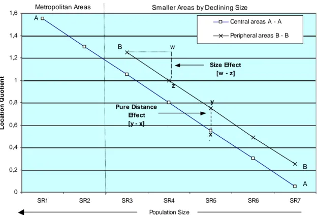
Figure 2 presents a perfectly symmetrical and hierarchical distribution of economic activity as would be predicted by Christallerian central place theory and the effects of spatial competition for demand-oriented commodities. We would a priori expect to find this kind of pattern for most high-order producer services. The sensitivity of the activity to city-size (agglomeration economies) is given by the height of the first (left-hand) value and the slope of the curves. Activities that are very sensitive to city-size will start with a high value and have a steep slope.

The sensitivity to distance (or rather to the proximity of a metropolitan area) is given by the distance between curves A and B, where B-B represents the (shorter) curve for urban areas located beyond an hour’s drive of a metropolitan area. In the case of Figure 2, curve B lies systematically above curve A, signifying (for the idealised case portrayed here) that for any given city-size values will always be higher for peripheral urban areas located at some distance from a metropolitan area. We shall call this the “pure” distance effect. In this idealised case, this is equivalent to a distance-protection effect. We would thus expect this to be the case for most service sector activities where the delivery and/or consumption of the service require travel (by the consumer or supplier).

Figure 2 - Idealized Hierarchical Distribution

0 0,2 0,4 0,6 0,8 1 1,2 1,4 1,6 SR1 SR2 SR3 SR4 SR5 SR6 SR7 Population Size Loc a ti on Q uot ie n t Central areas A - A Peripheral areas B - B x b y z Pure Distance Effect [y - x] Size Effect [w - z]

Smaller Areas by Declining Size Metropolitan Areas A A B B w

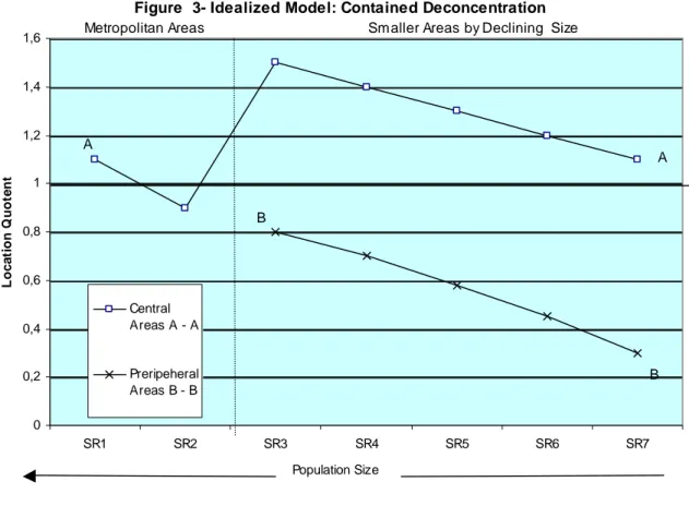
Figure 3 illustrates what we call “contained de-concentration” where, contrary to Figure 2, proximity to a metropolitan area is a positive factor. Curve B falls below A, signifying that for any given city size (below the metropolitan level) this industry will be less prevalent in peripheral SRs. We would expect this to hold for much of the manufacturing sector, specifically middle-range value added sectors that are sensitive to land and labour costs, and as such are “crowded-out” out of metropolitan areas. Note that in our example all values for curve B are below unity (1,0), but our hypothetical industry, even when located in peripheral SRs, nonetheless remains sensitive to agglomeration economies since its curve is downward-slopping. However, the mild slope of both curves, suggests that city-size (once “crowded-out”) is of less importance than proximity to a metropolitan area. The distance separating curves A and B signifies that the pure distance effect outweighs other effects.

Figure 4 represents the opposite case, what we shall call “unbounded de-concentration”, where industries react negatively both to city size and proximity (to a metropolitan area). B is above A, indicating that cities far from metropolitan areas are preferred, while the upward-moving slopes indicate that smaller cities are also favoured. In sum, the farther and the smaller the better, although we have stopped at rural areas, allowing the curves to flatten out. We should expect this pattern to describe traditional Weberian “weight loss” industries tied to “heavy” primary inputs that are most cheaply available in remote (non-metropolitan) locations. In the Canadian case, the pulp and paper industry immediately springs to mind.

D

M

The database is drawn from Canadian census data for 1971 and 1996. Canada is divided into 382 geographic units, which distinguish between urbanised and non-urbanised areas 5. The database comprises employment numbers for 142 distinct economic sectors for each of the 382 spatial units. Two 'geographies' were combined to arrive at the 382 distinct units. On the one hand, the 152 urban areas (25 CMAs, 115 CAs and 12 CSDs with over 10,000 inhabitants in 1991 6) were identified according 1991 boundaries. All data for 1971 and 1996 were adjusted to these boundaries. By the same token, data covering the entire territory of Canada by Census Division (290 census divisions (CDs)) were adjusted to 1991 territorial boundaries. To create a single database, data for urban areas were subtracted from data for the CDs within which they are located.

5

1991 population figures have been used to select urban areas. 6

Figure 3- Idealized Model: Contained Deconcentration 0 0,2 0,4 0,6 0,8 1 1,2 1,4 1,6 SR1 SR2 SR3 SR4 SR5 SR6 SR7 Population Size L o c a ti on Q uot e n t Central Areas A - A Preripeheral Areas B - B A B A B

Metropolitan Areas Smaller Areas by Declining Size

Figure 4- Idealized Model: Unbounded Deconcentration

0 0,2 0,4 0,6 0,8 1 1,2 1,4 1,6 SR1 SR2 SR3 SR4 SR5 SR6 SR7 Population Size Lo c a ti o n Q uot ie nt Central Areas A - A Peripheral Areas B - B A A B B

In cases where an urban area overlaps a number of CDs, the CDs were first aggregated, and the urban area variables subtracted from the values for the aggregated area. The result of these operations is a total of 382 spatial units (SUs), 152 of which are 'urban' and 230 and 'rural'.

The employment data for 1971 are defined according to the 1970 Standard Industrial Classification (SIC) while the 1996 data are defined according to the 1981 SIC. In order to make the two series compatible, it has been necessary to aggregate sectors: the result is that there are 142 compatible sectors that can be analysed from 1971 to 1996. We aggregated the 142 sectors into 18 economic sectors (see Annex 2). This classification is based upon the 15 sector classification used by Coffey and Shearmur (1996), but with a more detailed subdivision of manufacturing (3 sectors instead of 1) and producer services (2 sectors instead of 1).

Following from our general model, our spatial classes are defined as follows for Canada. On the one hand

• Metropolitan area: a CMA of over 500,000 inhabitants in 1991

• Urban area: a CMA, CA or CSD of over 10,000 inhabitants in 1991

• Rural areas: all areas that are not urban areas. It should be noted that rural areas can contain towns, but these are necessarily smaller than 10,000 inhabitants

and on the other

• Central areas: all areas within approximately one hour's drive (or 100 to 150 km) of a metropolitan area. Account has been taken of the highway infrastructure, the spatial extent of the metropolitan area, and the characteristics of the area being classified. Thus, the central areas do not necessarily form perfect rings around metropolitan areas

• Peripheral areas: All areas not classified as central or metropolitan

These classifications lead to the following definition of Synthetic Regions (SR’s) for Canada:

SR1: metropolitan areas of over 1 million inhabitants

SR2: metropolitan areas of between 500,000 and 999,999 inhabitants Central (located within a hour’s drive of SR1 or SR2)

SR3c: central urban areas of between 100,000 and 499,999 inhabitants SR4c: central urban areas of between 50,000 and 99,999 inhabitants SR5c: central urban areas of between 25,000 and 49,999 inhabitants SR6c: central urban areas of between 10,000 and 24,999 inhabitants SR7c: central rural areas

Peripheral (located beyond an hour’s drive of SR1 or SR2)

SR3p: peripheral urban areas of between 100,000 and 499,999 inhabitants SR4p: peripheral urban areas of between 50,000 and 99,999 inhabitants SR5p: peripheral urban areas of between 25,000 and 49,999 inhabitants

SR6p: peripheral urban areas of between 10,000 and 24,999 inhabitants SR7p: peripheral rural areas

At this point, it is important to emphasise that all data are by place of residence. This should be borne in mind when interpreting results since it is quite possible that actual jobs are located in SUs other than the place of residence. This is of particular relevance to SUs adjacent to metropolitan areas, which are in the rural central class (SR7c), and maybe to certain peripheral spatial units from which workers seasonally migrate. This caveat does not invalidate our results, but will influence our interpretations. Location quotients were calculated for sector employment in each SR. The analysis is not based upon mean values of the location quotients but on location quotients calculated for each SR in its entirety. Thus:

E

E

e

e

LQ

















=

∑

∑

LQ

a xi

e = employment in sector x in spatial unit i of synthetic region a a

i

e = total employment in spatial unit i of synthetic region a x

E

E

Following from the location quotient (LQ) results, six descriptive statistics were equally calculated:

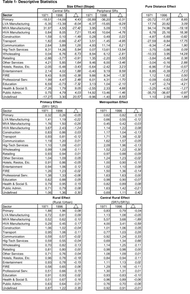
Size Effect: The slope of the curve linking LQs of urban areas of a given type (central or peripheral) between classes SR3 and SR6, assuming unit distance between adjacent classes. Metropolitan areas and rural areas are excluded. Since the largest urban areas are to the left of the figure, a positive result (i.e., positive correlation between city size and LQ) is associated with a downward sloping curve.

Pure Distance Effect: The mean difference between the value of LQs for central and peripheral SRs in the same class, again for that part of the curve falling between SR3 and SR6. A positive result means that curve A (central) lies above B.

Metropolitan Effect: Ratio of the highest SR1 or SR2 (metropolitan) LQ value to the mean value of all other urban SRs.

Primacy Effect: The ratio of the LQ value of SR1 to SR2.

Rural Effect: The ratio of the mean value of rural LQs to urban LQs. Central Rural Effect: The ratio of the LQ value of SR7c to SR7p.

R

For reasons of space, our visual results are limited to nine industrial classes (Figures 5 through 12). The figures for the service sector focus on private “tradable” services, which can be consumed or delivered over some distance, and thus have some locational flexibility. The results for retailing, personal services, public services and other services are, however, included in the descriptive statistical results (Table 1).

Manufacturing

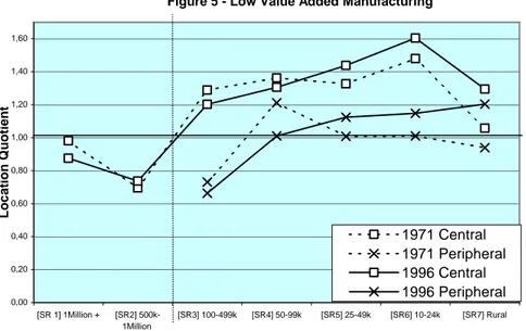
The results for low value added manufacturing (Figure 5) come very close to the idealised unbounded de-concentration model (Figure 4), with however a major caveat. On Figure 5, the periphery curve (B) falls below the central curve and not above. In other words, this sector tends to flee large cities; but it does not necessarily flee central locations. Proximity to large urban centres remains a positive factor for low value added manufacturing. The chief sectors which, proportionately, are more often found in peripheral locations are, not unsurprisingly, public administration, the primary sector, and transportation (Table 1). For these sectors, the pure distance effect in 1996 is negative (curve B falls above A). For low value added manufacturing, the negative impact of city size appears to have grown between 1971 and 1996 (increasing negative value for the city-size effect), both in central and peripheral locations. By the same token, both the metropolitan and primacy effects, already weak for the former, have declined further (Table 1). This is truly a sector which prefers (and increasingly so) to locate in small cities. However, the distance effect remains strong, and has even slightly increased. In sum, recalling our earlier discussion on ‘crowding out’ and the rationale for small and medium-sized cities, these are typically industries that seek out low cost labour and land markets, but nonetheless wish to remain within easy reach of a major metropolis. The evidence for Canada suggests that the latter effect continues to loom large. For any given city size (below 500k), central locations are clearly preferred. The distance effect looms even larger for medium value added manufacturing. Figure 6 is an almost perfect representation of our idealised contained de-concentration model (Figure 3). Indeed, the distance separating the peripheral and central curves is even greater than that posited in our idealised model 7.

7

Note that on Figure 6 the upper limit for LQ values is higher than for other figures, indicating an exceptionally high concentration of this sector in certain location; in central non-metropolitan locations in this instance. Figure 7 equally allows for LQ values above 1,60. All other figures are drawn on the same scale.

Table 1- Descriptive Statistics

Size Effect (Slope) Pure Distance Effect

Central SRs Peripheral SRs Sector 1971 1996 1971 1996 1971 1996 Primary -18,51 -14,09 4,43 -35,89 -36,20 -0,31 -20,72 -11,87 8,85 LVA Manufacturing -5,35 -13,39 -8,04 -6,37 -15,65 -9,28 17,74 20,82 3,09 MVA Manufacturing 31,97 4,55 -27,42 3,95 5,09 1,15 94,14 74,96 -19,18 HVA Manufacturing 0,84 8,05 7,21 15,40 10,64 -4,76 6,78 25,16 18,38 Construction 1,59 0,10 -1,49 0,28 0,49 0,22 -4,87 -5,69 -0,82 Transport 1,82 -0,66 -2,47 3,51 -1,45 -4,95 -27,59 -9,84 17,75 Communication 2,64 3,89 1,26 4,93 11,14 6,21 -9,34 -7,44 1,90 Hig-Tech Services 8,31 14,26 5,94 0,07 13,61 13,54 -3,75 -3,66 0,09 Wholesaling 0,04 6,76 6,73 8,94 6,12 -2,81 -10,33 3,95 14,28 Retailing -2,86 -3,77 -0,91 1,35 -2,20 -3,55 -3,84 -3,46 0,38 Other Services 4,21 5,85 1,64 9,46 6,00 -3,46 -3,04 -0,16 2,88

Hotels, Restos, Etc. -2,05 -5,48 -3,43 -5,64 -2,42 3,23 -6,96 -7,54 -0,57

Entertainment 2,14 4,02 1,88 -0,40 9,19 9,59 6,85 -0,39 -7,23

FIRE 9,43 9,05 -0,38 9,66 8,34 -1,32 1,12 1,62 0,50

Professional Serv. 1,99 4,47 2,48 6,01 4,31 -1,70 -0,09 -0,63 -0,54

Education 6,59 -0,73 -7,32 3,13 1,04 -2,10 1,47 -2,74 -4,21

Health & Social S. -7,26 1,79 9,05 -2,55 2,33 4,88 -3,25 -4,52 -1,27

Public Admin. 0,75 4,79 4,03 14,92 13,46 -1,46 -35,70 -36,67 -0,97

Undefined -17,27 3,30 20,57 -9,96 -1,40 8,55 1,10 2,99 1,88

Primacy Effect Metropolitan Effect

(SR1/ SR2) Sector 1971 1996 1971 1996 Primary 0,32 0,26 -0,05 0,62 0,82 0,19 LVA Manufacturing 1,41 1,19 -0,22 0,66 0,55 -0,12 MVA Manufacturing 1,76 1,50 -0,26 0,45 0,42 -0,03 HVA Manufacturing 3,67 2,43 -1,24 1,14 1,22 0,08 Construction 0,83 0,86 0,03 1,17 1,04 -0,13 Transport 0,93 0,81 -0,12 1,71 1,39 -0,32 Communication 1,19 1,20 0,01 1,62 1,57 -0,05 Hig-Tech Services 1,10 1,09 -0,01 2,09 1,96 -0,13 Wholesaling 0,99 1,09 0,11 1,52 1,22 -0,30 Retailing 0,93 0,94 0,01 0,97 0,88 -0,09 Other Services 1,04 1,09 0,05 1,24 1,23 -0,02

Hotels, Restos, Etc. 0,91 0,86 -0,05 1,00 0,90 -0,10

Entertainment 0,94 1,06 0,12 1,02 1,10 0,08

FIRE 1,26 1,23 -0,02 1,50 1,36 -0,14

Professional Serv. 1,38 1,33 -0,06 1,63 1,63 0,00

Education 0,82 0,88 0,05 0,98 0,90 -0,07

Health & Social S. 0,79 0,95 0,15 0,82 0,89 0,08

Public Admin. 0,71 0,79 0,08 1,63 1,42 -0,21

Undefined 1,06 1,36 0,30 0,69 1,11 0,42

Rural Effect Central Rural Effect

(Rural /Urban) (SR7c/SR7p) Sector 1971 1996 1971 1996 Primary 1,88 1,96 0,08 0,83 0,79 -0,04 LVA Manufacturing 0,72 0,81 0,09 1,13 1,08 -0,05 MVA Manufacturing 0,52 0,62 0,10 5,57 3,68 -1,89 HVA Manufacturing 0,29 0,45 0,17 4,00 3,41 -0,59 Construction 1,06 1,02 -0,04 1,01 1,06 0,05 Transport 0,95 1,06 0,11 0,77 1,03 0,26 Communication 0,59 0,57 -0,02 0,92 1,24 0,33 Hig-Tech Services 0,59 0,55 -0,04 0,69 1,34 0,66 Wholesaling 0,70 0,82 0,13 1,14 1,25 0,11 Retailing 0,81 0,80 0,00 0,98 0,98 0,00 Other Services 0,71 0,76 0,04 1,08 1,09 0,01

Hotels, Restos, Etc. 0,96 0,78 -0,18 0,84 0,94 0,11

Entertainment 0,93 0,78 -0,15 1,11 1,13 0,02

FIRE 0,58 0,65 0,06 1,29 1,18 -0,11

Professional Serv. 0,51 0,66 0,15 1,30 1,31 0,01

Education 0,91 0,93 0,02 0,93 0,83 -0,10

Health & Social S. 0,51 0,67 0,16 0,96 0,89 -0,06

Public Admin. 0,63 0,64 0,01 0,76 0,70 -0,06

Figure 5 - Low Value Added Manufacturing 0,00 0,20 0,40 0,60 0,80 1,00 1,20 1,40 1,60 [SR 1] 1Million + [SR2] 500k-1Million [SR3] 100-499k [SR4] 50-99k [SR5] 25-49k [SR6] 10-24k [SR7] Rural Synthetic Regions Locat ion Quot ient 1971 Central 1971 Peripheral 1996 Central 1996 Peripheral

Figure 6 - Medium Value Added Manufacturing

0,00 0,50 1,00 1,50 2,00 2,50 [SR 1] 1Million + [SR2] 500k-1Million [SR3] 100-499k [SR4] 50-99k [SR5] 25-49k [SR6] 10-24k [SR7] Rural Synthetic Regions Loc a ti on Q uot ie nt

Clearly, distance (from a major metropolis) remains an essential factor in the location decisions of a wide range of manufacturing industries. The results reconfirm (yet again) the robustness of the one-hour threshold, at least for the sectors contained in this class. The weight of the (positive) distance effect has declined somewhat between 1971 and 1996, but nonetheless remains very high (higher than for any other class of industries). The weak (and stable) metropolitan effect also signifies that these industries continue to shun large metropolitan areas (crowding-out). The major change has occurred in the city-size effect for central (non-metropolitan) locations, which has almost entirely disappeared (Table 1). A look at Figure 6 reveals that while the curve for central locations (between SR3 [100-499k] and SR7 [rural]) was systematically downward sloping in 1971, this is no longer so in 1996. In other words, within the central business service shed (surrounding large metropolitan areas), city size is no longer a major consideration. What counts is proximity to the metropolis. This lends credence to the hypothesis, referred to earlier, that IT does not reduce the need for business travel to and from the metropolis.

Figure 7 - High Value Added Manufacturing

0,00 0,20 0,40 0,60 0,80 1,00 1,20 1,40 1,60 1,80 2,00 [SR 1] 1Million + [SR2] 500k-1Million [SR3] 100-499k [SR4] 50-99k [SR5] 25-49k [SR6] 10-24k [SR7] Rural Synthetic Regions Locat ion Quot ient 1971 Central 1971 Peripheral 1996 Central 1996 Peripheral

The results for high value added manufacturing (Figure 7) are again very close to the idealised contained de-concentration model, but with an important caveat. The highest LQ values are found in the largest metropolitan areas, and this has not changed significantly between 1971 and 1996. Note the very high (although declining) primacy effect. Our results also suggest that the pure distance effect has increased between 1971 and 1996, and has also become more systematic. For any given

(non-metropolitan) city-size, LQ values in 1996 are always significantly higher in central than in peripheral locations. As for the previous figure, once outside the metropolis, proximity to the metropolis appears to matter more than city size. But, unlike the previous category, the strongest point of attraction remains the metropolis itself. This suggests a dual location pattern, analogous to the front office / back office distinction for producer services. The highest value added and knowledge intensive activities within this sector locate in the metropolis, while the more standardised and land-extensive activities locate in smaller cities nearby, specifically in cities in the 25-49k range in the Canadian case. For example, for the aerospace industry (included in this sector), research intensive activities would locate in the metropolis while more assembly-line type functions (or subcontractors) might locate in nearby smaller cities.

Services

Figures 8 through 10 show results for three classes of high-order producer services. All three show regular hierarchical patterns, with systematically downward sloping curves, close to the ideal model posited in Figure 2. Clearly, central place theory is not dead. However, agglomeration economies appear to far outweigh the pure distance effect.

City size matters more than pure location (i.e., distance from a large metropolis). The slope is particularly steep for the most information-intensive services (Figure 8), with a precipitous decline below the half-a-million (population) threshold. What is perhaps most striking is the stability of the curves over the twenty-five year period. These sectors are highly concentrated in the largest urban centres with little indication of major change over time. A slight trend to de-concentration is nonetheless perceptible. The LQ values for the highest urban class decline slightly in all three cases (especially for FIRE: Figure 10). The stability of the patterns is equally reflected in the descriptive statistics. Declines in the metropolitan and primacy effects are minor. Professional and high-tech producer services continue to register the highest metropolitan effect. On the whole, the city-size effect remains strong for all three classes, and has even notably increased for high-tech producer services 8.

8

The precipitous rise and subsequent decline in the LQ values for the peripheral 10-24k class (SR6p) is largely explained by the oil exploration boom (and later bust) in smaller Alberta cities. During the boom, these cities attracted numerous technical consulting and engineering firms.

Figure 8- High-Tech Producer Services 0,00 0,20 0,40 0,60 0,80 1,00 1,20 1,40 1,60 [SR 1] 1Million + [SR2] 500k-1Million [SR3] 100-499k [SR4] 50-99k [SR5] 25-49k [SR6] 10-24k [SR7] Rural Synthetic Regions Locat ions Quot ient s 1971 Central 1971 Peripheral 1996 Central 1996 Peripheral

Figure 9 - Professional Producer Services

0.00 0.20 0.40 0.60 0.80 1.00 1.20 1.40 1.60 [SR 1] 1Million + [SR2] 500k-1Million [SR3] 100-499k [SR4] 50-99k [SR5] 25-49k [SR6] 10-24k [SR7] Rural Synthetic Regions Locat ion Quot ient

Figure 10 - Finance, Insurance, Real Estate [FIRE] 0,00 0,20 0,40 0,60 0,80 1,00 1,20 1,40 1,60 [SR 1] 1Million + [SR2] 500k-1Million [SR3] 100-499k [SR4] 50-99k [SR5] 25-49k [SR6] 10-24k [SR7] Rural Synthetic Regions Locat ion Quot ient

The results for the entertainment sector (Figure 11) are somewhat different. Almost no slope was visible in 1971, with however a noticeable (but small) positive pure distance effect (see also Table 1). This suggests the spatial behaviour of a consumer-oriented non-tradable service, present in all locations. However, the pattern appears be changing, albeit slowly. For both central and peripheral (non-metropolitan) locations, the city-size effect has increased significantly, as has the primacy effect and, consequently, the LQ value of the largest urban class. The distribution is becoming more hierarchical over time, closer to the three previous figures, suggesting that the influence of agglomeration economies is growing, and that this is increasingly a tradable service. As for the three previous industries, the pure distance effect (proximity to a metropolis) no longer appears to be a major factor. It is location in a large metropolis that counts.

The results for wholesaling (Figure 12) are different again. A pure protective (negative) distance effect is visible in 1971, but has since been reversed (Table 1). Medium-sized peripheral cities (specifically those above 100k) played a significant role (LQ above unity) as wholesaling centres in 1971, a role that they appear to be losing. All peripheral urban areas have seen their LQs fall. The chief beneficiaries of this change are small and medium-sized cities falling within a one hour’s drive of a metropolis (especially in the 50-99k range).

Figure 11 - Entertainment 0,00 0,20 0,40 0,60 0,80 1,00 1,20 1,40 1,60 [SR 1] 1Million + [SR2] 500k-1Million [SR3] 100-499k [SR4] 50-99k [SR5] 25-49k [SR6] 10-24k [SR7] Rural Synthetic Regions Locat ion Quot ient 1971 Central 1971 Peripheral 1996 Central 1996 Peripheral Figure 12 - Wholesaling 0,00 0,20 0,40 0,60 0,80 1,00 1,20 1,40 1,60 [ SR 1] 1M illion + [ SR2] 500k-1M illion [ SR3] 100-499k [ SR4] 50-99k [ SR5] 25-49k [ SR6] 10-24k [ SR7] Rural Synthetic Regions Location Q uotient

The results for 1996 suggest a movement toward the contained de-concentration model, with however an important difference. In this case, the higher 1996 results for (non-metropolitan) central urban areas suggest a centripetal movement from peripheral to central urban areas, rather than simply a crowding out from metropolitan areas. The wholesaling sector is increasingly behaving like space-extensive manufacturing activities that seek out inexpensive locations close to large urban centres. In sum, this suggests a centralising movement at the level of the whole system, but a (contained) decentralisation movement inside the ‘central’ core (recall Figure 1). For wholesaling, the effects of IT have probably been to permit greater scale economies, notably in management, storage, and marketing (increasing the attraction of central locations), but the corresponding growing space requirements have in turn increased crowding-out pressures. Perhaps no case better exemplifies the multifaceted nature of the impacts we have been trying to measure, for here we appear to observe centralisation at one level and de-centralisation at another.

C

Our results, based on Canadian data for 1971 to 1996, suggest that the location of economic activity largely continues to follow predictable patterns, consistent with theory and recent literature on industrial location. Both distance (proximity to large urban centres) and city size remain good predictors of location patterns for most industrial classes, both in manufacturing and the service sectors. These results largely confirm earlier work and other studies. Patterns have remained very stable over the twenty-five year period studied, especially for higher order producer services. There is little indication that agglomeration economies have weakened over time or that spatial distributions are less hierarchical. Quite the contrary, in some cases such as wholesaling and entertainment observed, location patterns are becoming more hierarchical and more sensitive to agglomeration economies and central locations.

The “pure” effects of distance (as distinct from hierarchical city-size effects) remain important for manufacturing. Manufacturing plants may locate outside large urban areas (especially those falling in the low to medium value added range), but do not locate very far away. The approximate one-hour threshold (100 to 150 km from a major metropolis) has remained very robust over time as a predictor of the relative spatial concentration of manufacturing activity. The introduction of new information technology (IT) does not appear to have significantly altered this reality, at least not over the time period studied. The weight of the distance threshold seems, in fact, to have increased for high value added manufacturing. Businessmen (or women) and consultants must still travel to and from large metropolitan areas by car or other means

of transport. Goods must still be transported. IT does not change this. Our results should thus come as no surprise.

What is surprising is that some should have believed (or still believe) that this particular phase of technological innovation marks a dramatic break with past spatial trends. There is nothing in recent data for Canada or other nations to indicate a break in long-term urbanisation and spatial trends 9. Again, this is entirely consistent with our analysis and results, and should surprise no one. Others as well have noted that the announced “revolutionary” impacts of recent technological change are much exaggerated (Ghemawat, 2001; Gordon, 2000), although not specifically addressing the issue of industrial location. Regional scientists can equally rest assured that distance continues to matter, and that space, geography, and location are not about to magically disappear as important factors in the understanding of human behaviour.

R

Cairncross, F., 2001, The Death of Distance 2.0. How the Communications Revolution Will Change Our Lives. New York: W.W. Norton & Co.

Coffey, W. J. and M. Polèse, 1988, “Locational shifts in Canadian employment, 1971-1981, decentralisation versus decongestion”, The Canadian Geographer 32(3): 248-255.

Coffey, W. J. and R. Shearmur, 1996, Employment Growth and Change in the Canadian Urban System, 1971-1994. Working Paper No. 2, Canadian Policy Research Network, Ottawa.

Gasper, J. and E. Glaeser, 1998, “Information technology and the future of cities”, Journal of Urban Economics 43: 136-156.

Ghemawat, P., 2001, “Distance still matters: The hard reality of global expansion”, Harvard Business Review (September) 131-147.

Glaeser, E. L., 1998, “Are cities dying?”, Journal of Economic Perspectives 12(2): 139-160.

Gordon, R. J, 2000, “Does the ‘New Economy’ measure up to the great inventions of the past?”, Journal of Economic Perspectives 14(4): 49-74.

Graham, D. and N. Spence, 1997, “Competition for metropolitan resources: The “crowding out” of London’s manufacturing industry”, Environment and Planning A 29: 459-484.

9

Canadian metropolitan areas and ‘central’ locations, as defined here, continue to grow at a faster rate (in terms of employment and population) than the rest of the nation (Shearmur 2001).

Henderson, J. V., 1997, “Medium sized cities”, Regional Science and Urban Economics 27: 583-612.

Ingram, G. K. 1998, “Patterns of metropolitan development: What have we learned?”, Urban Studies 35(7): 1019-1035.

Kotkin, J., 2001, The New Geography. How the Digital Revolution is Reshaping the American Landscape. New York: Random House.

McNiven, C., H. Puderer, and D. James, 2000, “Census Metropolitan Areas and Census Agglomeration Influenced Zones (MIZ): A Description of the Methodology” Geography Working Paper Series, No. 2000-02. Statistics Canada, Geography Division, Ottawa.

Polèse, M., and E. Champagne, 1999, “Location matters: Comparing the distribution of economic activity in the Mexican and Canadian urban systems”, International Regional Science Review 22(1): 102-132.

Quigley, J. M., 1998, “Urban diversity and economic growth”, Journal of Economic Perspectives 12(2): 127-138.

Shearmur, R., 2001, Economic Development in Canadian Peripheral Regions. A Statistical Overview. Research Report, INRS-UCS, Montreal. Available on line at:

www.inrs-ucs.uquebec.ca

A

1: D

CMA

CA

Census Metropolitan Area (CMA)

A census metropolitan area (CMA) is a very large urban area (known as the urban core) together with adjacent urban and rural areas (known as urban and rural fringes) that have a high degree of social and economic integration with the urban core. A CMA has an urban core population of at least 100,000, based on the previous census. Once an area becomes a CMA, it is retained as a CMA even if the population of its urban core declines below 100,000. All CMAs are subdivided into census tracts. A CMA may be consolidated with adjacent census agglomerations (CAs) if they are socially and economically integrated. This new grouping is known as a consolidated CMA and the component CMA and CA(s) are known as the primary census metropolitan area (PCMA) and primary census agglomeration(s) [PCA(s)]. A CMA may not be consolidated with another CMA.

Census Agglomeration (CA)

A census agglomeration (CA) is a large urban area (known as the urban core) together with adjacent urban and rural areas (known as urban and rural fringes) that have a high degree of social and economic integration with the urban core. A CA has an urban core population of at least 10,000, based on the previous census. However, if the population of the urban core of a CA declines below 10,000, the CA is retired. Once a CA attains an urban core population of at least 100,000, based on the previous census, it is eligible to become a CMA. CA’s that have urban cores of at least 50,000, based on the previous census, are subdivided into census tracts. Census tracts are maintained for CA’s even if the population of the urban cores subsequently falls below 50,000. A CA may be consolidated with adjacent CA’s if they are socially and economically integrated. This new grouping is called a consolidated CA and the component CAs are called primary census agglomerations (PCA’s).

ANNEX 2: 142 Industrial sectors, 18 Sector Aggregation

Aggregated Class Sectors Aggregated Class Sectors

Primary 1 agriculture Communication 71 radio and televison broadcasting

2 forestry 72 telephone services

3 hunting and fishing 73 telepgraph services

4 metallic mines 74 postal services

5 coal mines LVA 75 electricity

6 petrol and natural gas LVA 76 gas distribution

7 non metallic minerals LVA 77 water distribution

8 oil wells and 'other mining services' LVA 78 other public utilities

Low Value Added (LVA) 9 meat and poultry Wholesale 79 food wholesale

10 fish processing 80 ironmongery - wholesale

11 fruit and vegetables 81 other wholesale

12 milk Retail 82 food retail

13 mills and animal food 83 various merchandise retail

14 bread 84 tire retail

15 other foods 85 gas stations

16 drinks 86 car dealers

17 tobacco 87 car maintenance and repair

Medium Value Added (MVA) 18 tires, rubber etc… 88 shoe shops

MVA 19 plastics 89 men's wear shops

Low Value Added (LVA) 20 shoes, leather etc… 90 women's wear shops

21 carpets 91 clothing shops

22 various textiles 92 ironmongers

23 clothing 93 furniture shops

24 wood transformation 94 electrical repair shops

MVA 25 furniture 95 pharmacies

LVA 26 paper 96 bookshops and stationers

Communication 27 printing 97 florists

LVA 28 metal transformation 98 jewels and jewel repair

LVA 29 metal products 99 spirit (alcohol) shops

MVA 30 machines 100tobacco and other shops

High Value Added (HVA) 31 business machines FIRE 101banks

HVA 32 aeronautics 102other credit organisations

Middle Value Added (MVA) 33 cars 103stock brokers

34 truck bodies 104investment companies

35 car parts 105insurance

36 rolling stock 106insurance and real estate agents

37 ships and vessels 107real estate managers

38 other transport equipment Education 108day care and establishments for annex care

39 small electical products 109primary and secondary schools

40 large electrical products 110art, professional, and non-university post seconda

41 lighting products 111universities and colleges

42 radios and televisions 112libraries

HVA 43 telecommunications equipment & micro-electronics 113teaching and related services

MVA 44 industrial electrical equipment Health and Social Services 114hospitals

MVA 45 electrical wires and cables 115doctors, surgeons and dentists

MVA 46 other electrical products 116para-medical practitioners

Low Value Added (LVA) 47 non metallic mineral products 117diagnostic services

48 oil and coal products 118other health related services

49 fertilisers Entertainment 119cultural organisations

50 plastics and resins 120cinemas

HVA 51 pharmaceutical products 121film production and distribution

LVA 52 paint and varnish 122entertainment, leisure, golf, billiards, bowling…

LVA 53 soap and cleaning products 123theatres and shows

MVA 54 personal hygiene products Other Services 124temping agencies

LVA 55 industrial chemical products High-tech producer services 125computer services

LVA 56 other chemical products Other Services 126security, investigation, and other business service

HVA 57 professional and scientific equipment Professional Services 127accounting

MVA 58 other manufacturing Professional Services 128marketing and advertising

Construction 59 construction High-tech producer services 129architects and engineering consultants

Transport 60 air transport Professional Services 130legal

61 services auxiliary to air transport High-tech producer services 131management consultants

62 rail transport Other Services 132personal services

63 maritime transport Hotels, Restaurants, Etc. 133hotels and motels

64 services to maritime transport 134boarding houses

65 trucking, removal and storage services 135camp sites

66 urban transport and inter-urban coach transport 136restaurants

67 taxis and other transport Other services 137other services

68 road maintenance Public Administration 138federal administration

69 services auxiliary to transport 139provincial administration

70 warehousing 140local administration

141foreign governments