To link to this article
: DOI: 10.1103/PhysRevE.82.036321
URL :
http://link.aps.org/doi/10.1103/PhysRevE.82.036321
This is an author-deposited version published in:
http://oatao.univ-toulouse.fr/
Eprints ID: 5430
To cite this version:
Willis, Ashley P. and Hwang, Yongyun and Cossu, Carlo Optimally amplified
large-scale streaks and drag reduction in the turbulent pipe flow. (2010)
Physical Review E , vol. 82 (n° 3). pp. 036321-1-036321-11. ISSN 1539-3755
O
pen
A
rchive
T
oulouse
A
rchive
O
uverte (
OATAO
)
OATAO is an open access repository that collects the work of Toulouse researchers
and makes it freely available over the web where possible.
Any correspondence concerning this service should be sent to the repository
administrator: [email protected]
!Optimally amplified large-scale streaks and drag reduction in turbulent pipe flow
Ashley P. Willis
*
and Yongyun Hwang†Laboratoire d’Hydrodynamique (LadHyX), École Polytechnique, 91128 Palaiseau, France
Carlo Cossu‡
Institut de Mécanique des Fluides de Toulouse (IMFT), 31400 Toulouse, France and Département de Mécanique, École Polytechnique, 91128 Palaiseau, France
The optimal amplifications of small coherent perturbations within turbulent pipe flow are computed for Reynolds numbers up to one million. Three standard frameworks are considered: the optimal growth of an initial condition, the response to harmonic forcing and the Karhunen-Loèvesproper orthogonal decompositiond analysis of the response to stochastic forcing. Similar to analyses of the turbulent plane channel flow and boundary layer, it is found that streaks elongated in the streamwise direction can be greatly amplified from quasistreamwise vortices, despite linear stability of the mean flow profile. The most responsive perturbations are streamwise uniform and, for sufficiently large Reynolds number, the most responsive azimuthal mode is of wave number m = 1. The response of this mode increases with the Reynolds number. A secondary peak, where
mcorresponds to azimuthal wavelengths lu+<70–90 in wall units, also exists in the amplification of initial conditions and in premultiplied response curves for the forced problems. Direct numerical simulations at Re = 5300 confirm that the forcing of m = 1 , 2 and m = 4 optimal structures results in the large response of coherent large-scale streaks. For moderate amplitudes of the forcing, low-speed streaks become narrower and more energetic, whereas high-speed streaks become more spread. It is further shown that drag reduction can be achieved by forcing steady large-scale structures, as anticipated from earlier investigations. Here the energy balance is calculated. At Re= 5300 it is shown that, due to the small power required by the forcing of optimal structures, a net power saving of the order of 10% can be achieved following this approach, which could be relevant for practical applications.
DOI:10.1103/PhysRevE.82.036321
I. INTRODUCTION
The nature of laminar-turbulent transition, and of the structure of turbulence in pipe flow, is a subject that has interested generations of fluid dynamicists since the pioneer-ing work of Reynolds f1g. Laminar pipe flow sthe
Hagen-Poiseuille flow solutiond is linearly stable, but subcritical transition to turbulence is observed at Reynolds numbers as low as<2000. A key mechanism in the transition process is played by the lift-up effect f2,3g consisting of the strong
amplification of the energy of streamwise streaks that evolve from streamwise vortices. These streaks are narrow elon-gated regions where the streamwise velocity is larger or smaller that the average at the same distance from the wall. The large amplification of the streaks by the lift-up mecha-nism is related to the strong non-normality of the linearized Navier–Stokes operatorf4–6g. Optimal perturbations, which
maximize the energy amplifications, have been computed for most of the canonical laminar shear flows, where it is found that streamwise uniform structures are the most amplified. The maximum amplification of initial conditions, and re-sponses to harmonic and stochastic forcing have been found to scale such as Re2, Re4, and Re3, respectively f6–9g. For
laminar pipe flow, the most amplified streamwise uniform
modes are those of azimuthal wave number m = 1 f10–12g,
decreasing monotonically with increasing m, and the result-ing streaks are significantly unstable when of sufficient am-plitudef13g.
Coherent streaky motions also exist in the turbulent pipe. The existence of streaks in the buffer layer with a mean spanwise spacing of <100 wall units has been well docu-mented for the boundary layer f14–16g and for pipe flows
f17,18g. Coherent streaky structures exist also at much larger
scales, of the order of several pipe radii, R. Recently it has been realized that these structures can be very longsat least <8R to 16Rd, and contribute to half of the total turbulent kinetic energy and Reynolds stressf19,20g. Contrary to other
canonical turbulent flows, for the case of the turbulent pipe relatively little is known on the spanwisesazimuthald struc-ture of these coherent large-scale strucstruc-tures.
While early computations of optimal growths and re-sponses to stochastic forcing f21–23g have considered the
turbulent mean flow as a base flow, the molecular viscosity was included in the equations for the coherent perturbations. An externally imposed eddy turnover time had to be included in the optimization process. More recent analyses of the tur-bulent plane channel flowf24–26g, boundary layer f27g and
Couette flowf28g have included the effect of the eddy
vis-cosity in the linearized equations, in the spirit of Ref.f29g. In
this approach the eddy turnover time need not be enforced, but is an output of the optimization process. Following this approach, two preferred spanwise wavelengths are found for the amplification of streamwise uniform streaks, for suffi-ciently high Reynolds numbers. The firstslz<3h to 4h for *[email protected]
plane channel flowd scales in outer units si.e., with the chan-nel half-width hd, and the maximum amplifications increase with the Reynolds number. The second preferred spanwise length, which scales in inner swalld units, is found at l+ <100, in good accordance with the scales of the buffer layer cycles. Here milder energy amplification of initial conditions is found. These results strongly suggest that the mean lift-up effect is involved as an essential part of the mechanisms that permit the sustainance of turbulent coherent structures.
When streaks are of finite amplitude they may support the amplification of secondary perturbationsf30,31g that lead to
their breakdown, and to the refueling of streamwise vorticity necessary to sustain the streaksf32,33g. This self-sustained
process is christened in the emergence of nonlinear saddle solutions f34,35g and unstable periodic orbits f36g. Many
unstable nonlinear solutions have also been found for pipe flow f37,38g, where a positive Lyapunov exponent is
dis-played in the turbulent regimef39g. These “exact” solutions
f40g, which are believed to provide a structure to the
sub-critical transition process f41g, typically have few unstable
eigenvalues and associated modes, while they are attracting in all other directions in phase space. It has therefore been conjectured that transitional flow spends significant periods of time in the neighborhood of a few of these nonlinear so-lutions, and that therefore the lowest order statistics could be retrieved by averaging over the exact solutions. This rational framework has been boosted by the experimental observation of the velocity field bearing resemblance to exact nonlinear traveling wave solutionsf42g. Exciting phase space portraits
of the transitional regime are becoming available for the plane Couette flowf43g.
It is currently not clear how to extend the dynamical sys-tems approach into the régime of developed turbulence. At large Reynolds numbers, exact solutions typically have high wave numbers, implying an unrealistic number of repetitions of the structure in space. Progress is being made with respect to this spatial dependence, with the discovery of localized counterparts to the infinitely extended solutionsf44g. Other
periodic solutions have been continued to high Reynolds numbersf45g. A different but serious problem is that, while
capturing the typical features of turbulence near the wall, exact solutions do not exhibit the large dissipation of turbu-lence in the central region of the flow. It is this dissipation that leads to flattened mean profiles of the flow and strong deceleration of the core region for pipe flow. This slow core is clearly present in the observations off42g. While
dissipa-tion occurs on small scales in the central region, however, coherent streaks certainly are present. A myriad of solutions exhibiting streaks is now available for pipe flowf46g, but it
is not yet clear how to determine which best characterize turbulence. Toward this end, in the present study the eddy viscosity is invoked to help reveal on which length scales the most important structures occur, those associated with energy production through amplification, and who’s presence may otherwise be masked by the dissipative eddies.
In addition to its potential relevance for understanding the structure of turbulent flows, the analysis of optimal energy amplifications is also relevant for flow control. In the laminar boundary layer, for instance, the forcing of nearly optimal streaks has been used to stabilize the base flow to
Tollmien-Schlichting wavesf47–49g and delay transition to turbulence
f50g. That large-scale coherent streaks can be effectively
am-plified in the turbulent boundary layerf51,52g has opened the
way for their use in separation control in industrial applica-tionsf53g. Furthermore, a few studies f54,55g have shown
that by forcing large-scale streamwise vortices, viscous drag can be reduced in the plane channel flow. However, in these studies the cost of the control action has not been evaluated, and it is therefore unclear if a net power saving can be achieved. In this study, the advantage of forcing optimal structures is that the energy required for the forcing is mini-mized, reducing the cost of the control.
The scope of the present investigations is therefore to an-swer the following questions: what are the optimal energy amplifications and responses to forcing sustained by the mean turbulent flow in a pipe? Structures of which wave-lengths are most amplified? And, how do these amplifica-tions and their structure change with Reynolds number? De-spite its ubiquity in practical applications, these results are not yet available for turbulent pipe flow. A linear model is presented in Sec. II. Linear results sSec.IIId, based on the
eddy-viscosity model, here and for the planar geometries, are yet to be compared with simulations of “real” turbulence, i.e., in full resolved simulationsSec.IVd. In other words, do
the optimal streaks predicted by the linear eddy-viscosity model compare well to artificially forced streaks computed in direct numerical simulation? As simulations in the pres-ence of turbulpres-ence are inherently nonlinear, what is the effect of finite amplitude forcing on these coherent streaks? Finally, we are interested in the influence of artificially forced finite amplitude streaks on the drag. Can the mean drag be reduced in the presence of large amplitude streaks? Is a net power saving, including the cost of the control, achievable, and if so, what is the best performance?
II. BACKGROUND
A. Turbulent base flow and eddy viscosity
Consider the incompressible flow of a viscous fluid of kinematic viscosity n in a circular pipe of radius R. The bulk velocity Ub smean streamwise speedd is assumed constant. Lengths are nondimensionalized by R and velocities by
Ucllam= 2Ub, the center-line speed for laminar flow of the same bulk velocity f12,38,56,57g. The usual Reynolds number
based on the mass flux is defined as Re= 2UbR /n. At suffi-ciently large Reynolds numbers the flow is turbulent and the turbulent mean flow profile preserves invariance in the span-wise directionu, the streamwise direction x, and in time t. The mean flow velocity is written U = Usydex, where y = 1 − r is the dimensionless distance from the boundary wall and
ris the radial coordinate. In complement to this “outer” scal-ing, convenient for measuring large-scale properties, to de-scribe near-wall structure it is commonplace to also define units via the friction velocity ut2= n]yUuy=0, based on the shear near the wall. The wall units of length and time are then n / utand n / ut
2
, respectively. Variables nondimensional-ized on this “inner” scaling bare the superscript + in the following, and the wall-Reynolds number is defined Ret = utR /n.
If, as a first approximation, the Boussinesq eddy viscosity is used to model the turbulent Reynolds-stresses, then the streamwise component of the Reynolds-averaged momentum conservation reads
1 Re
S
1
r+ ]r
D
snT]rUd = ]xP, s1dwhere the total effective viscosity is nTsyd=1+Esyd and Esyd is the eddy-viscosity, normalized such that at the wall nTs0d=1, i.e., the kinematic value is attained. We denote by
B= −]xP, the averaged streamwise pressure gradient neces-sary to maintain the prescribed mass flux.
For Esyd we use the convenient expression originally sug-gested for pipe flow by Cess f58g, later used for channel
flows by Reynolds and Tiedermanf59g, then by many others
f21,24,25g: Esyd =1 2
H
1 + k2Rˆ2Bˆ 9 f2y − y 2g2s3 − 4y + 2y2d2 3F
1 − expS
− yR ˆÎ
Bˆ A+D
G
2J
1/2 −1 2. s2dThe mean streamwise velocity Usyd in equilibrium with this radially dependent eddy viscosityfEq. s2dg is easily inverted
from the mean averaged momentum Eq. s1d, and matches
very well experimental observations. Here, Rˆ =Re/2, Bˆ=2B. The fitting parameters A+= 27 and k= 0.42 have been up-dated to improve the match with recent observations inf60g.
B. Equations for the small coherent perturbations to the turbulent base flow
We now take the state F =sU, Pd, solution of Eq. s1d, as a
ssteadyd base flow and consider small coherent scorrelated when ensemble-averagedd perturbations, w=su, pd, to F in the presence of a coherentscorrelatedd force f and/or coher-ent initial conditions u0. Note that F is understood to be the turbulent mean state for f = 0 and u0= 0.
The equations governing the coherent perturbations re-quire modeling of the Reynolds stresses to be closed. Rey-nolds and Hussain f29g discussed the eddy viscosity as a
simple closure model, finding that it compared well for small-amplitude perturbations. Linearizing the closed equa-tions, following f24–29g, the equation governing
small-amplitude coherent perturbations is ]tu + ur]rUex+ U]xu = − =p + 1
Re= ·fnTsyds¹u + ¹u Tdg
+ f. s3d
These perturbations also satisfy continuity, = · u = 0. The ex-plicit components for the viscous term are given in Appendix A.
Exploiting the rotational and the streamwise translational invariance of the system, one may expand the perturbations in Fourier modes wsr,u, x ; td=oamfˆamsr;tdeisax+mud, wherea and m are the streamwise and azimuthal wave number re-spectively. Substitution into Eq.s3d gives
]tfˆamsr;td = LamsFdfˆam+ fˆamsr;td, s4d where Lamis the linear operator acting on the Fourier mode
fˆamsrd. The problem may be considered for each mode in-dependently, and the subscripta, m is dropped in the follow-ing. The spanwise and streamwise wavelengths for each per-turbation are given by lu= 2p / m and lx= 2p /arespectively in units of R.
C. Optimal growth and response to forcing
Three properties of the linearized system are now exam-ined. They are the optimised growth of initial conditions, the optimised response to harmonic forcing, and the response to stochastic forcing. Standard definitionsssee, e.g., f6,61gd are
briefly restated below for the present context.
Optimal growth in time over all possible nonzero initial conditions uˆ0, for a particular a, m mode, is given by the function Gsa,m;td ; max uˆ0Þ0 iuˆstdi2 iuˆ0i2 , s5d
and the maximum achieved over all times is Gmaxsa, md ;maxtGsa, m ; td. Here fˆ=0, and the energy norm used is iuˆi2;s1/Vde
Vu · udV.
For harmonic forcing, fˆ = f˜eiVft, and accompanying
re-sponse, uˆ = u˜ eiVft, the optimal response is given by
Rsa,m;Vfd ; max
f
˜Þ0 iu˜i2
if˜i2. s6d
The maximum over all frequencies Vf is Rmaxsa, md = maxVf Rsa, m ; Vfd.
Finally, the response to a stochastic force is usually con-sidered in the discretized formshere radiallyd. Let fˆstd be the discretized stochastic force vector, andk·l denote ensemble averaging. Following analyses f9,22,61–64g, the forcing is
assumed to have Gaussian probability density with zero av-eragesi.e., kfˆl=0d, isotropic sequal variance on all the three componentsd and delta-correlated in space and time, kfˆstdfˆHst
8dl=Idst−t8d, where the superscript H denotes the Hermitian transpose. The amplification of the stochastic forc-ing is then measured by the variance of the response:
Vsa,md ; trhC`j, s7d
where C`=kuˆuˆHl is the covariance matrix for the response in the limit t → `. This covariance matrix is computed by solv-ing an algebraic Lyapunov equationssee Appendix Bd. The eigenfunction decomposition of the Hermitian matrix C`is known as the Karhunen-Loève sKLd or proper orthogonal decomposition sPODd. The ratio of its real and positive ei-genvalues, sn, to the variance V =onsnrepresent the relative contribution to the variance from each orthogonal mode. The eigenfunction corresponding to the leading eigenvalue thus contributes most to the variance V. For details see f9,22,62–65g.
D. Numerical methodology
The linear operator appearing in Eq. s3d must be
dis-cretized in order to compute the optimal growths and the responses described above. Some attention must be paid to difficulties introduced by the cylindrical geometry, and full details of the methods are given in Appendix B. Here we note the general approach and convergence of the results.
A Chebyshev-collocation method on up to N = 250 radial points was used to calculate up to 2N − 3 eigenvectors and eigenvalues for the linear system fEq. s3dg. The optimal
growth code, which requires only these eigenvectors, eigen-values and weights for calculating norms, is a well validated code used for several previous studiesf25,27,28,66g. Results
for the optimal growth and the response to steady forcing were also verified by direct time stepping. At the largest Re= 106 the power spectral drop-off for the optimal modes was of eight orders of magnitude.
Responses from the linear model are compared with direct numerical simulations of the original Navier-Stokes equa-tions. The pipe flow code described inf67g has been used for
simulation of full turbulence subject to a forcing f. This time stepping code also uses a Fourier decomposition inu and x, but finite differences on a nonequispaced radial syd nine-point stencil. Time steps are controlled using information from a second-order predictor-corrector method. For most simulations presented, the radial spacings are drmin+ = 0.11,
drmax+ = 4.4 swall units n/utd. With dealiasing, du +
= 5.9, dx
+ = 9.4 at the boundary, in a domain L = 15sRd, L+= 2700. Veri-fication of these results is performed by calculation where the spacings above are respectively 0.08, 4.0, 3.9, 6.3 for L = 20. Simulations enforce a fixed mass flux, consistent with previous analysesf54,68g.
III. LINEAR AMPLIFICATION OF COHERENT STRUCTURES
A. Wave number dependence
We first consider the dependence of the optimal amplifi-cations on the streamwise and azimuthal wave numbers at the very large flux-Reynolds number of Re= 106 correspond-ing to Ret= 19 200. Figure1shows the dependence of Gmax,
Rmaxand V on m for the selecteda= 0 , 1 , 10, 100, 1000. It is clear from all plots that streamwise elongated structures, where lx. lu, are significantly amplified. The greatest growths are found for axially independent modessa= 0d, for which the curve provides an envelope over the results for nonzero a. The maxima on the a= 0 curves are for m = 1 azimuthal symmetry. The inset to Fig.1sbdshows that steady forcing is optimal for axially independent harmonic forcing,
a= 0, while for streamwise nonuniform perturbations, a non-zero forcing frequency is optimal. For the stochastic forcing at the optimal valuea= 0 , m = 1, it is found that the leading Karhunen-Loève mode dominates, representing 93% of the contribution to the total variance, as reported in the inset to Fig.1scd.
A secondary peak occurs in Gmax at a larger m corre-sponding to an azimuthal wavelength of lu+= 92swall units n / utd. Contrary to the optimal growth of initial conditions,
1 10 1 10 100 1000 10000 105 10000 1000 100 1 10 100 1000 λ+ θ Gm a x (α , m ) m α= 0 0.0001 0.01 1 100 10000 106 1 10 100 1000 10000 105 10000 1000 100 1 10 100 1000 1 100 10000 106 -1 -0.5 0 0.5 1 λ+ θ α = 0 α = 0 α = 1 m = 1 Rm a x (α , m ) m R (Ω f ) Ωf 0.01 0.1 1 10 100 1000 10000 1 10 100 1000 10000 105 10000 1000 100 1 10 100 1000 0.01 0.1 1 10 100 0 5 10 15 20 α = 0 m V (α , m ) σn (% ) n α = 0,m = 1 λ+ θ (a) (b) (c)
FIG. 1. sColor onlined Optimal energy growth of initial condi-tions Gmaxsad, optimal response to harmonic forcing Rmaxsbd and
variance of the response to stochastic forcing V scd for Ret
= 19200. Dependence on azimuthal wave number m, with corre-sponding wavelength in wall units lu+stop axisd, for selected values of the dimensionless streamwise wave numbera. Reference slopes
m−2 and m−1 sdotted linesd are shown in subfigures sbd and scd
respectively. The dependence of the optimal harmonic forcing am-plification Rsa,m=1;Vfd on the forcing frequency Vfis reported in
the insert of subfiguresbd for a=0 and a=1; Rmax= maxVfR. The
percentage contribution to the variance, 100sj/Vs0,1d, of the
re-sponse to stochastic forcing contained in the first 20 Karhunen-Loève modes is reported in the insert of subfigurescd.
no secondary peak is found in the optimal response to forc-ing. A closer examination of Figs.1sbdand1scdreveals that the Rmaxand V curves corresponding toa= 0 scale approxi-matively like m−2and m−1, respectively, for intermediate val-ues of m. A noticeable change of slope is found for valval-ues of
m corresponding to lu+<100. In plane channel flow, this power-law dependence has been explicitly related to the be-havior of geometrically similar optimal structures in the log-layerf26g. In the case of the response to forcing, primary and
secondary peaks occur in the deviations from this power-law behaviorf26g. This can be seen by considering the
premul-tiplied responses m2R
max and mV. A secondary peak at lu + = 73 is found in the premultiplied response curves fora= 0, shown in Figs.2sbdand2scd.
B. Reynolds number dependence
The spanwise optimal wave numbers, corresponding to the primary and to the secondary peak, do not change with Re when, respectively, scaled with outer and inner units. This can be seen in Fig. 2, where Gmax and the premultiplied
m2Rmax, mV computed for Re= 104, 105, and 106 scorre-sponding to Ret= 317, 2380, and 19 200, respectivelyd for
a= 0 are reported. While the premultiplied response to steady forcing is useful for showing deviations from the Rmax ,m−2 trend, the premultiplied stochastically forced case is arguably more representative of turbulence. When m is pre-sented on a log scale, equal area under the curve mV implies equal contribution to the total variance. Here, where the spanwise wave number is integer for pipe flow, all the pri-mary peaks are reached for m = 1 except for the premultiplied stochastic response at lower Ret; for Ret= 104, m = 2 is pre-ferred and the selection of m is very weak in mV for Re = 104 and lower. The secondary peak is always found at l
u + <70–90 for all the premultiplied responses. The primary and the secondary peaks, however, are not yet separated at Ret= 104, while they are for Ret= 105 and higher, in good accordance with the turbulent plane channel f24–26g the
boundary layerf27g.
The maximum responses, associated with the primary peaksa= 0, m = 1d increase with the Reynolds number, while
those associated with the secondary peak remain almost con-stant. The structure of the leading modes corresponding to
1 10 1 10 100 1000 10000 1 0.1 0.01 0.001 λθ Re= 104 105 106 m Gm a x (0 , m ) 10000 100000 1 10 100 1000 10000 1 0.1 0.01 0.001 λθ Re= 104 105 106 m m 2R m a x 106 100 1000 1 10 100 1000 10000 1 0.1 0.01 0.001 λθ Re= 104 105 10 6 m m V 1 10 0.0001 0.001 0.01 0.1 1 105 10000 1000 100 10 λ+ θ Re= 104 105 106 m+ Gm a x (0 , m ) 10−5 10 100 1000 0.0001 0.001 0.01 0.1 1 105 10000 1000 100 10 λ+ θ Re= 104 105 106 m+ (m +) 2R +m a x 10−5 10 100 0.0001 0.001 0.01 0.1 1 105 10000 1000 100 10 λ+ θ Re= 104 105 106 m+ m +V + 10−5 (a) (b) (c) (d) (e) (f)
FIG. 2. sColor onlined Dependence on the azimuthal wave number m and the corresponding azimuthal wavelength stop axisd of: the optimal energy amplification of initial condition Gmaxfsad and sddg, the premultiplied optimal response to harmonic forcing m2Rmaxfsbd and
sedg and of the premultiplied variance of the response stochastic forcing mV fsbd and sedg. Streamwise uniform sa=0d perturbations are considered for the selected Reynolds numbers Re= 104, 105and 106corresponding to Re
t= 317, 2830, and 19200. The responses, wave
numbers and wavelengths are scaled in outer units on the upper rowfsad, sbd, and scdg and in inner units in the lower row fsdd, sed, and sfdg.
FIG. 3. sColor onlined Linear optimal re-sponses to steady forcing for a = 0 and m = 1 , 2 , 4; Ret= 19200. Vectors: cross-stream
com-ponents of the input vector field. sColoredd con-tour levels: streamwise component of the output field sstreaksd. White fast-streaks, red/dark slow streaks.
the primary peak for optimal growth, for the response to steady and stochastic forcing, appear to be almost identical and remain the same over the entire range of Reynolds num-bers. Plotted in Fig. 3 are the leading modes for m = 1 , 2 , 4 sdata from the optimal harmonic forcing case at Re=106d. The optimal input consists of the expected large-scale streamwise vortices and the optimal output of large-scale streamwise streaks. Note that in this geometry, only modes of m = 1 can exhibit flow across the axis. The structures cor-responding to the secondary peak, which scale in inner units, are almost indistinguishable from those found in the plane channel and the boundary layerf25–27g and are therefore not
reported here.
IV. SIMULATION OF FORCED FINITE AMPLITUDE COHERENT STREAKS
A. Response to finite amplitude optimal steady forcing The optimal response predictions, described in the previ-ous section, were based on two main simplifying assump-tions:sad the effect of the uncorrelated motions was modeled with an isotropic eddy-viscosity andsbd coherent perturba-tions were assumed small. We now test the level of
approxi-mation implied in these assumptions by computing in full DNS the effective responses of the predicted optimal pertur-bations. In particular, we consider the response to the optimal steady large-scale forcing, the mode which is the most am-plified, and potentially the most relevant for passive flow control applications. The forcing term f is taken to be pro-portional to the mode f˜ that optimizes Rmax, obtained from the above linear analysis, for a= 0 and a given m. As the considered optimal forcing is steady, time averages can be easily calculated and the statistical convergence readily checked. The magnitude of the steady forcingifi is measured by the rms value, as before. The response of the flow in simulations is given by u¯sr,ud=kulx,t− U¯ srdxˆ, where U¯ srd =kulu,x,t is the mean flow in the absence of forcing. k·ls indicates averaging over the subscripted variables. Averages are taken over at least 2800R / Ucllamtime units. The DNSs are performed at Re= 5300, for which Ret= 180.
From Fig.4it is seen that the amplitude of the responses iu¯i depends linearly on the forcing for small forcing ampli-tudesifi. Small forcing can lead to large responses, in agree-ment with the linear eddy-viscosity model and, in the linear régime, the leading mode is m = 1, as expected. The response predicted by the linear eddy-viscosity model is Rmax= 2762 for m = 1 at this Re, while in the simulations, iu¯i/ifi is a factor 2 smaller than expected in the linear range. As the time-averaged mean flow for the unforced case, obtained from DNS, deviates very little from that given by Eqs.s2d
ands1d, this difference is most likely attributed to the
isotro-pic eddy-viscosity assumption. Similar considerations apply to the observation that the m = 4 mode is slightly more re-sponsive than the m = 2 mode in the linear regime.
For larger forcing amplitude, the amplitude of response saturates. For the m = 1 mode, this saturation begins when the amplitude AS of the associated coherent streaks is near to 19% of the center-line speed, where AS=
1
2smax u¯x− min u¯xd f69g. The responses to higher order optimal modes sm=2 and m= 4d saturate at larger forcing amplitudes ifi, and therefore
contain more energy iu¯i2 than the m = 1 mode, for suffi-ciently large forcing amplitudes.
In Fig.5, we report the finite amplitude coherent vortices and streaks induced by the steady forcing for, respectively, 0.01 0.1 0.0001 0.001 m=1 m=2 m=4 ||f || || ¯u ||
FIG. 4. sColor onlined Response to forcing in full simulation showing the linear régime and nonlinear saturation.ifi is the rms value. The isolated line is of slope 1 and squares correspond to the plots of Fig.5.
(a) (b) (c)
(d) (e) (f)
FIG. 5. sColor onlined Nonlinear responses to finite amplitude forcing for a = 0 and m = 1 , 2 , 4 from direct numerical simulation at Ret= 180.
Small forcing amplitudesupper rowd and moder-ate forcing slower rowd, corresponding to the marked squares in Fig.5.sad m=1, ifi=8.010−5; sbd m=2, ifi=1.410−5;scd m=4, ifi=8.010−5;sdd
m= 1,ifi=8.010−4;sed m=2, ifi=8.010−4;sfd m
= 4, ifi=2.510−4. Vectors: cross-stream
compo-nents of the forced velocity field.sColoredd con-tour levels: streamwise component of the output field sstreaksd. White fast-streaks, red/dark slow-streaks.
low and moderate forcing amplitudes for the three azimuthal modes m = 1, m = 2, and m = 4. From these figures, and by comparing them with the linear optimals reported in Fig.3, it is seen how, for increasing forcing amplitude, the low-speed streaks are more and more spatially concentrated, while high-speed streaks have a tendency to widen.
B. Influence on the drag
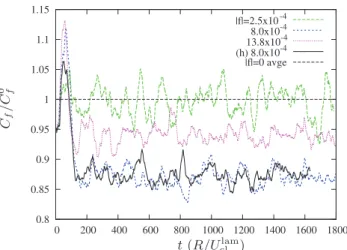
We now examine the influence of the forced finite ampli-tude streaks on the drag, always at Re= 5300scorresponding to Ret= 180d. Figure 6 shows time series for the instanta-neous Cf= 2sut/Ubd2in full DNS for three levels of optimal steady forcing of the m = 1, a= 0 mode. In wall units, the spanwise wavelength of the forced streaks for m = 1 is lu+ <1130, which extends by a factor greater than 2 the spac-ings considered in earlier investigations of the plane channel flow f54,55g. The horizontal line in Fig. 6 represents the baselinestime averagedd Cfin the absence of forcing. From this figure we see that indeed average drag reductions can be obtained also in the turbulent pipe flow. We have verified the accuracy of this result, in particular that no loss of the ob-served drag occursssolid lined, by performing an additional calculation at higher resolution smore than doubling the number of grid points, see Sec.II Dd.
In Fig. 7, the relative change for time averaged Cf is reported versus the forcing amplitude for the m = 1, m = 2, and m = 4 modes. Drag reduction is obtainable over a range of forcing amplitudes covering approximately one order of magnitude. Selecting the best forcing amplitude, the maxi-mum drag reduction achieved is 12.8% when forcing the m = 1 mode. It is reduced for higher modes, e.g., 10.4% for
m= 2slu+<565d and 4% for the mode m=4 slu+<280d. Forc-ing streaks at the near-wall peak mean spacForc-ing slu+= 100, corresponding to m<12d results in increased drag.
For this control strategy to be interesting for applications, the net power saved must be considered. The power
con-sumptionsper unit lengthd spent to maintain the desired con-stant volume flux of the turbulent flow is P =p8Cf in units rUcllam3R, and the control power spent sper unit lengthd to maintain the vortices is W =L1eu·fdV. The drag relative to the unforced case is then given by Cf/Cf0= P / P0, and the total relative net power consumption bysP+Wd/ P0. The per-centage net power saving is thus 100f1−sP+Wd/ P0g. From Fig. 7, where the relative drag and net power consumption are shown versus the forcing power, it is seen that the best net power saving corresponds to 11.1% and is obtained for the m = 1 mode. For this case, W is only 1.4% of P0. The response to forcing the large-scale mode is large, and as a result little energy is required to generate the prominent large-scale slow streak which affects the drag at the walls. The forcing of higher optimal modes results in smaller net power savingsse.g., at best 8.3% for m=2 and 3.3% for m = 4d.
The drag reducing mechanism appears to be consistent with that observed in plane channel flowf54,55g. Figure8sad
shows a snapshot of streamwise vorticity field in the absence of forced streaks. Intense small-scale quasistreamwise vorti-ces with lu+<100 appear irregularly but in the whole azi-muthal domain. These vortices, largely responsible for the turbulent skin friction f70g, are weakened when large-scale
streaks are artificially forced, and are almost suppressed from the high-speed streak region as seen in Figs.8sbdand8scd. In 0.8 0.85 0.9 0.95 1 1.05 1.1 1.15 0 200 400 600 800 1000 1200 1400 1600 1800 |f|=2.5x10⁻⁴ 8.0x10⁻⁴ 13.8x10⁻⁴ (h) 8.0x10⁻⁴ |f|=0 avge t (R/Ulam cl ) Cf / C 0 f
FIG. 6. sColor onlined Relative drag for several levels of steady forcing of the m = 1 mode from direct numerical simulation. At in-termediate levels of forcing the drag is reduced, falling below the average of the unforced caseshorizontal straight lined. The forcing can reduce the drag. The solid line is a higher resolution check at ifi=8.010−4. 0.8 0.9 1 1.1 1.2 1.3 0.0001 0.001 0.01 0.1 W/P0 Cf/Cf 0 (P+W)/P0 m=1 m=2 m=4
FIG. 7. sColor onlined Effect of forcing on the mean skin fric-tion, relative to the unforced casessolidd. Relative net power con-sumption including the work done by the force sdashedd. Black square corresponds toifi=8.010−4.
(a) (b) (c)
FIG. 8.sColor onlined Snapshots of the cross-stream distribution of the streamwise vorticity vxfield at a selected streamwise station
from direct numerical simulation.sad Streamwise vorticity in the absence of forcing.sb,cd Weakened and localized streamwise vor-ticity in the presence of the m = 1 , 2 steady forcing, corresponding to optimal drag reduction. Blue/dark intense vorticity, white no vortic-ity. Same color scales are used on all the subplots. Contour lines denote isolevels of the streamwise averaged velocity sthe forced streaksd.
the absence of this mechanism the drag would only increase due to distortion of the mean flow by the forcing. This drag, however, only appears to be large for moderate to large am-plitudes of the forcing, leading to the observed drag reduc-tion for intermediate forcing.
V. SUMMARY AND CONCLUSIONS
The first part of this investigation was dedicated to the computation of the optimal linear energy amplifications of coherent structures supported by the turbulent pipe mean flow. The problem formulation and the tools used in the analysis follow those of investigations of the turbulent plane channel flowf24–26g, Couette flow f28g, and boundary layer
flowf27g. In accordance with these investigations it is found
that, despite the turbulent mean flow is linearly stable, it can support the energy amplification of initial conditions and of harmonic and stochastic forcing. These energy amplifications have the expected characteristics of the lift-up effect, where vortices amplify streaks and the most amplified perturbations are streamwise uniform sa= 0d. For these streamwise uni-form structures, at sufficiently large Re, the maximum en-ergy amplifications are obtained for the m = 1 azimuthal mode. Furthermore, this large amplification increases with the Reynolds number. As observed in the Couette and plane channel flowf26,28g, for the three different calculations, the
initial value problem, response to harmonic forcing and most energetic Karhunen-Loève mode for stochastic forcing, the optimal inputs and outputs almost coincide.
A secondary peak is found in the Gmaxsm,a= 0d curves for the azimuthal mode corresponding to an azimuthal wave number lu+= 92, but only a change of slope in the
Rmaxsm,a= 0d, Vsm,a= 0d curves is noticeable at this lu + . The responses Rmaxand V of optimal harmonic and stochas-tic forcing, fora= 0 decrease with the azimuthal wave num-ber, with an approximate scaling of m−2and m−1respectively for intermediate m. For the plane channel flow, this inverse power dependence on the spanwise wave number has been related to the amplification of geometrically similar struc-tures in the log-layerf26g. To highlight the departure of the
optimal responses from the power-law trend, the premulti-plied responses m2R
max and mV have been considered. A secondary peak is then found at lu+= 73. This peak wave-length and the corresponding responses do not change with Reynolds number, provided that they are scaled in inner units, and that the Reynolds number is sufficiently large, so as to allow for a well defined inner-outer scale separation. The corresponding structures consist of streamwise uniform buffer-layer streaks and vortices.
The linear formulations we have used allowed a relatively straightforward computation of the linear optimal energy am-plifications. The advantage of this model, based on the tur-bulent eddy viscosity, is therefore its simplicity, while quan-titatively accurate predictions could be made with more sophisticated models. It is however important to verify that the predictions of the model, such as the order of magnitude of the growth of structures at large scale, or the fact that they more amplified than small-scale structures, are at least quali-tatively verified. We have therefore reported the results of
direct numerical simulations, where coherent structures have been artificially forced at the moderate Ret= 180. The opti-mal steady forcing of large-scale structuressm=1, m=2, and
m= 4d has been considered as these structures are the most
responsive, and therefore are not only easier to detect, but are potentially most interesting for control purposes. The main predictions of the linear model are qualitatively observed in the DNS: the low-m optimal perturbations show a very large response in the amplitude of induced streaks. For sufficiently small forcing amplitudes, the response to forcing is linear and the azimuthal symmetries of the forced modes are well preserved in the response. In this linear regime, the m = 1 mode is the most responsive. The agreement between the amplifications predicted by the linear model and the one ob-served in the DNS is only qualitative. The quantitative dif-ferences can probably be attributed to the very eddy-viscosity assumption and could probably be reduced by using a more realistic modeling of the Reynolds stresses. As coherent structures are strongly elongated in the streamwise direction, the isotropic eddy viscosity is gives only a first order approximation. At finite amplitudes of the coherent motions, the neglected interactions with the mean flow and the random turbulent field clearly become important f71g.
For larger forcing amplitudes, a saturation in the amplitude of the forced response is observed. The m = 1 mode is the first to saturate, at a considerable amplitude of almost 20% of the centerline velocity. For increasing amplitudes, the sym-metry between the high and low-speed streaks is progres-sively lost. Low speed streaks concentrate in smaller span-wise extensions, with slightly larger amplitude, while high-speed streaks widen and slightly decrease in amplitude. This asymmetry recalls the observed “real” unforced turbulent flowsf72g.
The exact relation existing between optimally amplified streaks and the coherent structures populating the “natural” sunforcedd turbulent pipe flow requires consideration. In the plane channel and Couette flows, the similarity of the span-wise scales selected by the linear mechanism and those ob-served in the actual turbulent flow is probably explained by the requirement that significant amplification is necessary for energetic turbulent processes to be self-sustained. What is currently not clear, because of the lack of experimental or numerical data, is if m = 1 is the dominating coherent mode at sufficiently large Re. Most of the investigations of large- and very-large scale coherent motions in the pipe flow f19,20,73,74g, have rather focused on the streamwise scales
of these motions. If these motions arise through a self-sustaining process, then the streamwise scales of the motion would be selected by processes related to the breakdown of the streaks. This process is missing in the present analysis. What can be said with the model, however, is which azi-muthal modes are most amplified for a streamwise scale se-lected by other stochastic processes. For instance, if one con-siders streamwise wavelengths ranging from lx= 16sRd sa <0.4d to lx= 6 sa<1d, then the most amplified structures vary from m = 2 to m = 5 modes at sufficiently large Re in the stochastic response. However, at even moderately low Rey-nolds numberse.g., Re=104corresponding to Ret= 317d, the azimuthal selection is weak and modes ranging from m = 1 to
integrated response. These predictions are compatible with recent results from direct numerical simulations at Ret = 150f75g where the most energetic POD modes are found
for the streamwise wavelength lx= 20sRd sthe computational box sized and for azimuthal modes ranging from m=2 to m = 7. Additional simulations or experiments would be highly desirable to examine the azimuthal structure of the most en-ergetic modes at larger Re.
One of the most relevant applications of the optimal per-turbations of the turbulent mean flows probably resides in flow control. The direct numerical simulations confirm that energy can be greatly amplified in a turbulent flow. An ob-jective of both theoretical and practical relevance is the re-duction of the power required to drive the constant mass flux through the pipe. Using optimal forcing, less than 2% of the power required to pump the sunforcedd flow, is required to induce modifications in the mean flow of the order of 20% of the centerline mean velocity. Previous numerical f54g and
experimentalf55g studies have shown that it is possible to
reduce the mean turbulent drag in the plane channel flow by forcing large-scale vortices with spanwise wavelength of <400–500 wall units. Here we have extended this result to pipe flow, where lu+<1200 wall units for m=1. Mean drag reductions of<13% are achieved by forcing this m=1 mode, while the drag reduction is reduced for reduced spanwise spacing. Inf54g the observed drag reduction was attributed
to the mean weakening of the circulation of quasistreamwise coherent vortices. This effect on the quasistreamwise vorti-ces is found in the present turbulent pipe flow. Our visual-izations show that the quasistreamwise vortices of the “natu-ral” buffer layer cycle are packed in the low-speed streak region, while they are essentially removed from the high-speed streak region.
At present it is not clear why the drag reduction reduces as the spanwise spacing is reduced. It is possible that for m = 2slu+<600d the reduced scale separation from that of the naturally occurring streaks slu+<100d causes the drag-reduction effect to be reduced. At spanwise separations greater than those possible at this Ret, where clear scale separation occurs, a plateau in the drag reduction is possible for separations greater than lu+<1200. However, if the great-est reduction continues to be observed for the larggreat-est pos-sible spacing, here m = 1, it may be conjectured that, rather than scaling in inner units, the mode that most reduces drag has an upper limit that depends on the geometry. Additional simulations or new experiments at much larger Ret could confirm or reject these conjectures.
We have also extended earlier investigations by comput-ing the net power savcomput-ing obtained by forccomput-ing the optimal coherent streaks. As these streaks are optimal, the power re-quired to force them is already almost minimized. Even at the considered low Reynolds number, the controlling streaks are forced with less than 2% of the power necessary to main-tain the base flow, and a net power saving of <11% is achieved with the m = 1 mode. For useful implementation of the method proposed in this study, the induction of rolls need not be efficient. For example, efficiency of 50%, still using only 4% of the driving energy, might be acceptable. Note also that, as the amplification of the forcing is expected to increase with increasing Re, the percentage of total power
used to force the streaks is predicted to decrease for increas-ing Re. In practice, induction of large-scale rolls is possible via passive actuators in laminar f49,50,76g and turbulent
flowsf51–53g. Although neither would reproduce the precise
details of forcing used here, linear optimals are known to be robust to perturbations of the system, and responses close to those seen here can be expected. An experimental verifica-tion of the proposed control strategy would of course be very welcome.
ACKNOWLEDGMENTS
We gratefully acknowledge financial support from the Eu-ropean Community’s Seventh Framework ProgrammesFP7/ 2007-2013d under Grant agreement No. PIEF-GA-2008-219-233.
APPENDIX A: RADIALLY-DEPENDENT VISCOSITY For the radially dependent effective viscosity, nTsrd, the viscous terms in Eq.s3d are given by
= ·fnTsrds=u + =uTdg = nT=2u + ]rnT·
3
2]rur ]ruu−1 ruu+ 1 r]uur ]xur+ ]rux4
, sA1d where =2u =3
¹2u r− 2 r2]uuu− ur r2 ¹2uu+ 2 r2]uur− uu r2 ¹2u x4
. sA2dAPPENDIX B: NUMERICAL CONSIDERATIONS Cumbersome differential operations in cylindrical coordi-nates, particularly given nT= nTsrd, mean that finding the Orr-Somerfield form for Eq.sB2d is not straight forward in this
geometry. Instead, for this study the continuity equation to-gether with Eq.s3d have been used directly in primitive
vari-able form, giving the generalized eigenvalue problem
Xfˆ = − sYfˆ , sB1d where fsr;td=fˆ srdest. Note that Y is singular, containing three zero boundary conditions and a zero right hand side for the continuity condition. Simplifications can be made by ob-serving that X is invertible, and that, as the s have real part strictly less than zero, Eq.sB1d can be written in the standard
form, s−1/sdcˆ =sX−1Ydcˆ . Standard LAPACK routines re-turn the leading eigenvalues along with a predicable number of infinite eigenvalues that are easily filtered. Excellent nu-merical stability is observed.
The continuity equation together with the linearized Eq. s3d and no-slip boundary conditions can be written in the
form
u = Vx,
]tx = Lx + Wf, sB2d
where x is an alternative representation for the state spacef. Conversion between the representations is performed by the action of V and W. This form is again familiar through the Orr-Somerfield formulation of the governing equations. Here, however, the eigenfunction decomposition is em-ployed. Matrix V has columns of eigenvectors uˆn and L = diagssnd, with the sn arranged in descending order. These matrices, along with the diagonal weight matrix M s.t.iui2 ;uHMu, are sufficient to calculate optimally growing initial conditions.
Consider the norm for x given by iui2= xHMˆ x;ixi2 =sx,xd, where Mˆ =VHMV. The optimal initial condition x
0
for growth at time t satisfies Gstd=sAx0, Ax0d/sx0, x0d =sA+Ax
0, x0d/sx0, x0d, where the transfer function for x is
A = etLand the adjoint can be shown in a few operations to be A+= Mˆ−1AHMˆ . The growth and initial condition can be
calculated by power iteration on the matrix A+A. This matrix
is straight-forward to evaluate when L is diagonal.
Calculation of the optimal harmonic forcing requires only minor alterations to the above. In this case one uses A =siVfI − Ld−1, which is again a diagonal matrix for L diag-onal.
For the stochastic response, it can be shown f65g that
C`= VG`VH, where G`solves the Lyapunov equation
LG`+ G`LH+ WWH= 0. sB3d
For W one may take the Moore-Penrose pseudoinverse of V. sSingularity of Y leads to fewer columns of eigenvectors than rows in V.dMATLABroutines are then available to solve Eq.sB3d.
f1g O. Reynolds,Proc. R. Soc. London 35, 84s1883d.
f2g H. K. Moffatt, in Proceedings of the URSI-IUGG Colloquium
on Atomspheric Turbulence and Radio Wave Propagation, ed-ited by A. Yaglom and V. I. TatarskysNauka, Moscow, 1967d, pp. 139–154.
f3g M. T. Landahl,J. Fluid Mech. 98, 243s1980d.
f4g S. C. Reddy and D. S. Henningson,J. Fluid Mech. 252, 209 s1993d.
f5g L. N. Trefethen, A. E. Trefethen, S. C. Reddy, and T. A. Driscoll,Science 261, 578s1993d.
f6g P. J. Schmid and D. S. Henningson, Stability and Transition in
Shear FlowssSpringer, New York, 2001d.
f7g L. H. Gustavsson,J. Fluid Mech. 224, 241s1991d.
f8g K. M. Butler and B. F. Farrell,Phys. Fluids A 4, 1637s1992d. f9g B. F. Farrell and P. J. Ioannou,Phys. Fluids A 5, 2600s1993d. f10g L. Bergström, Stud. Appl. Math. 87, 61 s1992d.
f11g L. Bergström,Phys. Fluids A 5, 2710s1993d.
f12g P. Schmid and D. S. Henningson,J. Fluid Mech. 277, 197 s1994d.
f13g O. Y. Zikanov,Phys. Fluids 8, 2923s1996d.
f14g S. J. Kline, W. C. Reynolds, F. A. Schraub, and P. W. Runsta-dler,J. Fluid Mech. 30, 741s1967d.
f15g J. R. Smith and S. P. Metzler,J. Fluid Mech. 129, 27s1983d. f16g J. C. Klewicki, M. M. Metzger, E. Kelner, and E. M. Thurlow,
Phys. Fluids 7, 857s1995d.
f17g M. K. Lee, L. D. Eckelman, and T. J. Hanratty s1974d. f18g B. U. Achia and D. W. Thompson, J. Fluid Mech. 81, 439
s1977d.
f19g K. C. Kim and R. Adrian,Phys. Fluids 11, 417s1999d. f20g M. Guala, S. E. Hommema, and R. J. Adrian,J. Fluid Mech.
554, 521s2006d.
f21g K. M. Butler and B. F. Farrell,Phys. Fluids A 5, 774s1993d. f22g B. F. Farrell and P. J. Ioannou,Phys. Fluids 5, 1390s1993d. f23g B. F. Farrell and P. J. Ioannou,Theor. Comput. Fluid Dyn. 11,
237s1998d.
f24g J. C. del Álamo and J. Jiménez, J. Fluid Mech. 559, 205 s2006d.
f25g G. Pujals, M. García-Villalba, C. Cossu, and S. Depardon, Phys. Fluids 21, 015109s2009d.
f26g Y. Hwang and C. Cossu, J. Fluid Mech. sto be publishedd. f27g C. Cossu, G. Pujals, and S. Depardon,J. Fluid Mech. 619, 79
s2009d.
f28g Y. Hwang and C. Cossu,J. Fluid Mech. 643, 333s2010d. f29g W. C. Reynolds and A. K. M. F. Hussain,J. Fluid Mech. 54,
263s1972d.
f30g F. Waleffe,Phys. Fluids 7, 3060s1995d.
f31g W. Schoppa and F. Hussain,J. Fluid Mech. 453, 57s2002d. f32g J. Hamilton, J. Kim, and F. Waleffe,J. Fluid Mech. 287, 317
s1995d.
f33g F. Waleffe, Stud. Appl. Math. 95, 319 s1995d. f34g M. Nagata,J. Fluid Mech. 217, 519s1990d. f35g F. Waleffe,Phys. Rev. Lett. 81, 4140s1998d.
f36g G. Kawahara and S. Kida,J. Fluid Mech. 449, 291s2001d. f37g H. Faisst and B. Eckhardt,Phys. Rev. Lett. 91, 224502s2003d. f38g H. Wedin and R. Kerswell,J. Fluid Mech. 508, 333s2004d. f39g N. V. Nikitin,Fluid Dyn. 44, 652s2009d.
f40g F. Waleffe,J. Fluid Mech. 435, 93s2001d.
f41g B. Eckhardt, T. Schneider, B. Hof, and J. Westerweel,Annu. Rev. Fluid Mech. 39, 447s2007d.
f42g B. Hof, C. van Doorne, J. Westerweel, F. Nieuwstadt, H. Faisst, B. Eckhardt, H. Wedin, R. Kerswell, and F. Waleffe, Science 305, 1594s2004d.
f43g J. F. Gibson, J. Halcrow, and P. Cvitanovic, J. Fluid Mech.
611, 107s2008d.
f44g T. M. Schneider, J. F. Gibson, and J. Burke,Phys. Rev. Lett.
104, 104501s2003d.
f45g D. Viswanath,Philos. Trans. R. Soc. London, Ser. A 367, 561 s2009d.
f46g C. C. T. Pringle, Y. Duguet, and R. R. Kerswell,Philos. Trans. R. Soc. London, Ser. A 367, 457s2009d.
f47g C. Cossu and L. Brandt,Phys. Fluids 14, L57s2002d. f48g C. Cossu and L. Brandt, Eur. J. Mech. B/Fluids 23, 815
s2004d.
f49g J. Fransson, L. Brandt, A. Talamelli, and C. Cossu,Phys. Flu-ids 17, 054110s2005d.
f50g J. H. M. Fransson, A. Talamelli, L. Brandt, and C. Cossu, Phys. Rev. Lett. 96, 064501s2006d.
f51g G. Pujals, C. Cossu, and S. Depardon, Sixth Symposium on
Turbulence and Shear Flow PhenomenasSeoul National
Uni-versity, Seoul, Korea, 2009d.
f52g G. Pujals, C. Cossu, and S. Depardon, J. Turbul. sto be pub-lishedd.
f53g G. Pujals, S. Depardon, and C. Cossu, Exp. Fluids sto be pub-lishedd.
f54g S. Schoppa and F. Hussain,Phys. Fluids 10, 1049s1998d. f55g G. Iuso, M. Onorato, P. G. Spazzini, and G. M. di Cicca,J.
Fluid Mech. 473, 23s2002d.
f56g S. A. Orszag and A. T. Patera,J. Fluid Mech. 128, 347s1983d. f57g M. Quadrio and S. Sibilla,J. Fluid Mech. 424, 217s2000d. f58g R. D. Cess, Westinghouse Research Report No. 8–0529–R24,
1958sunpublishedd.
f59g W. C. Reynolds and W. G. Tiederman,J. Fluid Mech. 27, 253 s1967d.
f60g B. J. McKeon, M. V. Zagarola, and A. J. Smits,J. Fluid Mech.
538, 429s2005d.
f61g B. F. Farrell and P. J. Ioannou,J. Atmos. Sci. 53, 2025s1996d. f62g B. Bamieh and M. Dahleh,Phys. Fluids 13, 3258s2001d.
f63g M. R. Jovanović and B. Bamieh, J. Fluid Mech. 534, 145 s2005d.
f64g P. Schmid,Annu. Rev. Fluid Mech. 39, 129s2007d.
f65g K. Zhou, J. Doyle, and K. Glover, Robust and Optimal Control sPrentice Hall, New York, 1996d.
f66g E. Lauga and C. Cossu,Phys. Fluids 17, 088106s2005d. f67g A. P. Willis and R. R. Kerswell,Phys. Rev. Lett. 100, 124501
s2008d.
f68g A. P. Willis and R. R. Kerswell, J. Fluid Mech. 619, 213 s2009d.
f69g P. Andersson, L. Brandt, A. Bottaro, and D. Henningson, J. Fluid Mech. 428, 29s2001d.
f70g A. G. Kravchenko, H. Choi, and P. Moin,Phys. Fluids A 5, 3307s1993d.
f71g Y. Lifshitz, D. Degani, and A. Tumin,Flow, Turbul. Combust.
80, 61s2008d.
f72g C. D. Tomkins and R. J. Adrian, J. Fluid Mech. 490, 37 s2003d.
f73g W. R. B. Morrison and R. E. Kronauer,J. Fluid Mech. 39, 117 s1969d.
f74g K. J. Bullock, R. E. Cooper, and F. H. Abernathy, J. Fluid Mech. 88, 585s1978d.
f75g A. Duggleby, K. S. Ball, and M. Schwaenen,Philos. Trans. R. Soc. London, Ser. A 367, 473s2009d.
f76g J. Fransson, L. Brandt, A. Talamelli, and C. Cossu,Phys. Flu-ids 16, 3627s2004d.