Nonlinear optimal large-scale structures in turbulent channel flow

Science Arts & Métiers (SAM)

is an open access repository that collects the work of Arts et Métiers Institute of

Technology researchers and makes it freely available over the web where possible.

This is an author-deposited version published in:

https://sam.ensam.eu

Handle ID: .

http://hdl.handle.net/10985/17882

To cite this version :

Mirko FARANO, Stefania CHERUBINI, Pietro DE PALMA, Jean-Christophe ROBINET - Nonlinear

optimal largescale structures in turbulent channel flow European Journal of Mechanics

-B/Fluids - Vol. 72, p.74-86 - 2018

Any correspondence concerning this service should be sent to the repository

Administrator :

[email protected]

Nonlinear optimal large-scale structures in turbulent channel flow

M. Farano

a,b,

*

, S. Cherubini

a

, P. De Palma

a

, J.-C. Robinet

b

a_{DMMM, Politecnico di Bari, Via Re David 200, Bari, Italy}

b_{DynFluid, Arts et Metiers ParisTech, 151 Bd. de l’Hopital 75013, France}

Keywords:

Nonlinear optimization Coherent structures Turbulent shear flows Hairpin vortices Large-scale streaks

a b s t r a c t

Coherent structures in turbulent shear flows take the form of packets of hairpin vortices reaching the outer region of the boundary layer along with streaks of different size, going from the near-wall to the outer region. The latter can be explained by the linear transient growth of the perturbations of the mean turbulent profile. Whereas, the former are recently found to be optimally-growing only in the presence of nonlinear effects, as ascertained for a turbulent channel flow at a low friction Reynolds number. The present work aims at investigating whether large-scale streaks can be optimally-growing in a nonlinear framework for a turbulent channel flow. Changing the friction Reynolds number from 180 to 590, the nonlinear optimal perturbation tends towards more robust large-scale streaks and vortical structures of smaller size. These streaks are generated by a coherent large-scale lift-up mechanism, acting as a source term in the energy balance, inducing a positive turbulent kinetic energy production at the outer scale. This indicates that the outer energy production peak arising between the two considered Reynolds numbers can be associated with the growth of optimal large-scale streaks, which represent a robust feature of turbulent channel flows.

1. Introduction

Turbulent flows are characterized by the chaotic dynamics of fluctuations around a statistically steady mean flow. Most of the efforts done in the last decades aimed at studying the turbu-lent regime by analysing the flow statistics [1], which are well characterized by well-defined and robust laws [2]. However, in addition to this chaotic dynamics, turbulent flows also appear to be populated by coherent structures, i.e. fluid motions highly coherent in space and lasting for a reasonable time. Unlike the chaotic fluctuations, which have a very low dynamical relevance, these coherent structures carry a large part of the flow momentum [3].

The first evidence of organized motion in turbulent flows was related to the presence of near-wall streaks [4], whose length and time scales expressed in terms of viscous quantities are invari-ant [5]. Several authors [6–8] have observed that the near-wall motion is self-sustained [8] due to the feedback of the secondary instability of the streaky structures onto the streamwise vortices able to generate them. Part of this self-sustained wall-cycle is based on the lift-up mechanism [9], which is a nonmodal mechanism able to induce O(1) streaks from vortices of O(1

/

Re). Such a linear, nonmodal mechanism can be explained by the non-normality of the Navier–Stokes operator linearized around the (statistically)

*

Corresponding author at: MMM, Politecnico di Bari, Via Re David 200, Bari, Italy.

E-mail address:[email protected](M. Farano).

steady mean flow, and can be easily retrieved by means of a linear transient-growth analysis [10]. In fact, optimally-growing perturbations can be employed to understand the features of the coherent motion in transitional and turbulent flows. As explained by Luchini [11], in highly non-normal shear flows, a randomly chosen small-amplitude initial disturbance will tend to produce an output coinciding almost entirely with the optimal perturbation. Extending this concept to the nonlinear framework, nonlinear transient-growth analyses have been found to recover optimal flow structures similar to those typically observed in transitional and turbulent flows, containing all of the basic elements of the self-sustained wall-cycle. In fact, in most of the cases, nonlinear optimal perturbations of laminar base flows [12–14] and turbulent mean ones [15] are composed of bent streaks and vortices, similar to the structures constituting the wall cycle.

Apart from the (now well established) wall cycle, recent studies have conjectured the existence of self-sustained Large Scale Mo-tion (LSM) [16–18] in the outer region of turbulent flows, charac-terized by the presence of elongated streaks whose wavelengths scale with the outer units (for instance, the spanwise and stream-wise spacings are of order of magnitude of 1

−

2h and 2

−

3h, respec-tively, as reported by Balakumar and Adrian [19] and Hwang and Cossu [16], where h is the half-height of a channel). Evidence of the self-sustained nature of such LSM has been provided by Hwang and Cossu [16], Hwang and Cossu [17], Rawat et al. [18], Hwang [20], Hwang and Bengana [21]. In these works, the Small-Scale Motion (SSM) has been damped using a Large Eddy Simulation (LES) with

an increasing value of the Smagorinsky constant. The observation that the LSM remains sustained even when the SSM was artificially dumped has led to the idea that large-scale streaks are regenerated by a (large-scale) self-sustained cycle similar to the wall one. In fact, similarly to the near-wall streaks, the occurrence of these structures can be easily linked to the lift-up mechanism acting at a large scale, as ascertained by several local linear transient growth analyses perturbing the turbulent mean flow (see [22–24]). These authors have found that optimal flow structures having a spanwise wavelength of the same order of magnitude of the outer length scale have indeed the form of large-scale streaks.

However, a global nonlinear optimization recently performed by Farano et al. [15] for a turbulent channel flow at Re_τ

=

180 has shown that, when the optimization is performed for a time scale associated with the LSM, the nonlinear optimal perturbations are characterized mostly by near-wall streaks and hairpin vortices populating the outer region. In particular, the streaky structures observed at the outer scale are very weak compared to both hairpin vortices and near-wall streaks, although it has been demonstrated that large-scale streaks can be self-sustained in turbulent flows. One possible explanation can be found in the friction Reynolds number used for those optimizations. In fact, at this rather low Reynolds number, the turbulent kinetic energy production in the outer region is overtaken by the dissipation [7,15], suggesting that the large scale streaks, generated by an energy production mechanism such as the lift-up, might be outscored by the growth of dissipative hairpin vortex structures. Whereas, at a larger Reynolds number allowing a net energy production at the outer scale [25], large-scale streaks might be optimal also in a nonlinear framework. The present work aims at investigating whether large-scale streaks can be optimally-growing in a nonlinear framework for a turbulent channel flow. Towards this aim, we have considered a moderately larger Reynolds number (Re_τ

=

590) compared to that considered in [15] (Re_τ

=

180), and following this work we have used a fully 3D nonlinear optimization to maximize the energy of perturbations of the turbulent mean flow. The results of this nonlinear optimization allow us to show the presence of an optimally growing oscillating streaky motion at the outer scale in a turbulent channel flow at Re_τ

=

590. These optimal flow structures are then compared to those at Re_τ

=

180. Clearly, being the optimizations limited to only two values of Re_τ, we do not aim at providing any quantitative dependence of the results on the Reynolds number. However, comparing the results at two different values of Re_τ might help understanding the physical mechanisms behind the formation of large-scale structures in turbulent flows.

2. Numerical methods

We consider the turbulent flow in a channel at moderate Reynolds number Re

=

Uch

/ν

, h being the half distance between the plates and Uc the centreline velocity of the mean velocity profile. When considering a turbulent flow, variables can be nor-malized using the half height h and the velocity Uc(referred to as ‘‘outer’’ units), or using the friction velocity u_τ

=

(µ

dU

/

dy

)

1_w/2 and the viscous length scale

ν/

u_τ (referred to as ‘‘inner’’ units). Hereafter, variables expressed in inner units will be labelled with the superscript+

, any other variable being normalized with respect to outer units. The friction velocity is used to define the friction Reynolds number Re_τ

=

u_τh

/ν

, which here is set to the two constant values, Re_τ

=

180 and 590, guaranteed by a constant pressure gradient. Computations are performed using the spectral-element code NEK5000 [26], with Legendre polynomial recon-struction of degree seven and second-order accurate Runge–Kutta time integration [27] with constant time step equal to∆t

=

0

.

013 for C180 and∆t

=

0

.

0001 for C590. Dirichlet boundary conditions for the three velocity components are imposed at wall, whereas pe-riodicity is prescribed in the streamwise and spanwise directions

(denoted with x and z, respectively, whereas y denotes the wall-normal direction). Details about the computational domain, as well as the number of grid points and the length of the cells are provided in Table 1. The domain lengths have been chosen following [1] for C180, and [25] for C590, who selected the domain sizes so that the two-point correlations in the streamwise and spanwise directions were close to zero at half of the domain size. Low- and high-order statistics (mean velocity and r.m.s. profiles), which have been validated with respect to those provided by Kim et al. [1] for C180 and Moser et al. [25] for C590, are reported in theAppendix.

2.1. Nonlinear optimization

The aim of this work is to compute optimal perturbations ca-pable of inducing a peak of kinetic energy in a finite time T when evolving nonlinearly over the mean flow. To describe the nonlinear evolution of perturbations of the mean turbulent velocity profile we use the following system of equations (NS′

):

∂

u′

∂

t

= −

u ′

· ∇

u′

−

u′

· ∇

U

−

U

· ∇

u′

− ∇

p′

+

1 Re

∇

2_u′

+ ∇ ·

τ

,

(1)

∇ ·

u′

=

0

,

where u′

₌

(u′

_{, v}

′

_{, w}

′ )T_{and p}′

represent the velocity and pressure perturbations of the mean turbulent velocity profile U(y), andτ

is the Reynolds stress tensor forcing the mean turbulent velocity profile, defined as the Reynolds average of u′

u′

. A DNS of the fully turbulent flow is used to compute the mean velocity profile as well as the Reynolds stress tensor (although they could be extracted from an existing database). Details of the derivation of Eqs.(1)are provided by Farano et al. [15].

We aim at maximizing the kinetic energy growth of perturba-tions u′

at a time T , the energy being defined as E(t)

=

{

u′ (t)

,

u′ (t)

} =

∫

V

(

u′2

+

v

′2

+

w

′2

)

(t)dV

,

(2) where V is the volume of the computational domain. The energy gain G(T )

=

E(T )

/

E(0) is maximized using a Lagrange multiplier approach in which the initial energy E0, along with the NS

′

equa-tions(1), are imposed as constraints using the Lagrange multipliers or adjoint variables (u′†

,

p†

, λ

). Following previous works focusing on nonlinear optimal perturbations of laminar base flows (see [28–

30]) and turbulent mean ones (see [15]), the optimization prob-lem is solved by direct-adjoint iterations coupled with a gradient rotation algorithm [31]. The iterative procedure is stopped when the relative variation between two successive direct-adjoint loops, e

=

(Gn

₋

_Gn−1₎

_/

_Gn_{is smaller than 10}−7_{, n being the iteration}

number. It is noteworthy that these optimizations require a high computational cost. In fact, depending on the selected target time, 40 to 80 direct-adjoint iterations are needed for achieving con-vergence for one set of parameters. Therefore, each optimization needs from 800.000 to 2.000.000 CPU hours on an IBM cluster Intel ES 4650, the computational time increasing remarkably with the Reynolds number.

3. Results

Firstly, DNSs of turbulent channel flow at Re_τ

=

180 (C180) and Re_τ

=

590 (C590) have been performed. The mean velocity profile as well as the root mean square (r.m.s.) of the velocity field are found to be coincident (within plotting accuracy) with those reported by Kim et al. [1] and Moser et al. [25] (see theAppendix). A visualization of the flow structures is provided inFig. 1, showing the vortical structures identified by the second invariant of the velocity gradient tensor (known as Q-criterion, see [32]). For C180

Table 1

Simulation parameters for the two cases considered in the present work.

Reτ Re ∆x+ _∆z+ _∆y+ max ∆y + min Lx Lz Nx×Ny×Nz C180 180 3300 12 7 4.4 0.05 4π 2π 192×160×160 C590 590 12450 9.7 4.8 7.2 0.05 2π π 384×256×384

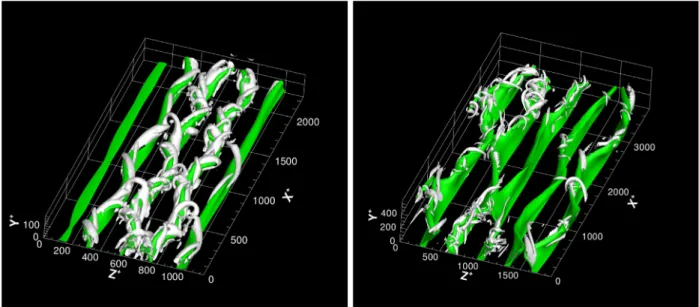
Fig. 1. Instantaneous isosurfaces of the second invariant of the velocity gradient tensor, Q-criterion (Q/Qmax=0.025), coloured by the streamwise velocity: left, C180; right,

C590.

(left), several hairpin-like vortical structures can be observed [33]. On the other hand, from a qualitative point of view, one can notice the loss of coherence of the vortical structures when increasing the Reynolds number (C590 right). In both cases, looking at the instantaneous vortical structures, no clear evidence of LSM can be observed, as also remarked by Hwang and Cossu [16].

To show the presence of a streaky LSM, one can average the perturbation flow field in the streamwise direction. The result of the streamwise averaging procedure over a single snapshot extracted from the DNS is shown of Fig. 2 for C180 (left) and C590 (right). The top frames provide a close-up of the wall region (y+

≤

50), whereas the bottom ones extend up to the centre of the channel, with axes scaled in outer units. As one can notice, the near-wall region is characterized by an alternation of small-scale low- and high-velocity streaks. Their spanwise spacing is of the order of magnitude of 100 viscous length units, although we do not measure exactly the mean value reported in the literature [3,25] since a single snapshot is used here for streamwise-averaging. Moving away from the wall, similar structures are observed, whose size grows towards the centreline of the channel, reaching an average spacing of order of magnitude of h, as reported in the lit-erature [19]. This feature is observed at both considered Reynolds numbers (compare left with right frames) but it is clearer at higher Re_τ.

3.1. Nonlinear optimal structures

Nonlinear optimizations are performed with target time T

=

31

.

12 (corresponding to T+

_≈

305 for C180 and T+

_≈

874 for C590, respectively). In order to allow the growth of large-scale motion, this target time has been chosen approximately equal to the eddy turnover time at the centre of the channel, defined as the ratio between the turbulent kinetic energy and the dissipation rate, k

/ϵ

(see [10]). Therefore, we anticipate that optimal structures maximizing the growth at the outer scale will be obtained, as in [10,15].Fig. 3provides a visualization of the optimal

perturbations computed for C180 (E0

=

10−2, left frame) and

C590 (E0

=

7

.

5

×

10−4, right frame). In both cases the initial

energy has been chosen as the smallest energy providing a well converged finite amplitude solution (see the discussion in the Appendix of [15]). For both values of the Reynolds number, we have verified that the optimal disturbances keep a similar structure as long as the initial energy is sufficiently high to trigger nonlinear effects. Both frames show that the optimals at target time are composed of elongated negative streaks (green) with spanwise spacing

≈

h (in inner units, h+

₌

Re_τh) along with a family of local-ized vortical structures (grey), among which hairpin-like vortices can be recognized. These vortical structures are often observed as coherent structures populating the log layer and characterizing the outer motion of wall-bounded turbulent flows [16–18,20,21,35]. However, one may notice some qualitative differences between the optimal flow structures at the two considered Reynolds num-bers. In particular, for the largest value of the Reynolds number, the streamwise perturbation isosurfaces representing the streaks appear to extend towards the centre of the channel, whereas the vortical structures appear to decrease their size, in agreement with what has been observed in the DNS snapshots shown inFig. 1.

For analysing the nonlinear optimal perturbations from a quan-titative point of view, the dominating wavelengths within the perturbed flow are extracted by inspecting their premultiplied spatial energy density spectra versus y+(shaded contours), shown inFigs. 4and5for the streamwise and spanwise directions, k+

x and k+

z, respectively. Such figures also provide the premultiplied energy density spectra obtained by the DNS results (solid lines), for comparison. We recall that the premultiplied spectrum kx,zE(kx,z) is defined such that the area under the curve in the plane log(kx,z)

−

kx,zE(kx,z) represents the energy content [36]. The spectra corre-sponding to Re_τ

=

180 and Re_τ

=

590 are shown on the left and right column, respectively; the top, middle, and bottom rows providing the streamwise (Euu), wall-normal (Evv), and spanwise

(E_ww) energy densities. One can observe that, increasing Re_τ(from left to right), all the DNS spectra extend to higher values of y+

Fig. 2. Streamwise-averaged perturbation of the mean flow for C180 (left) and C590 (right), on a z−y plane scaled in outer units (bottom) as well as a close-up scaled in

inner units (top). Blue (red) contours indicate negative (positive) values of the streamwise velocity perturbations. (For interpretation of the references to colour in this figure legend, the reader is referred to the web version of this article.)

Fig. 3. Shape of the optimal perturbations at t=T : isosurfaces of negative streamwise velocity perturbation (u′_/u′

max =0.45, green) and of the second invariant of the

velocity gradient tensor, Q-criterion (Q/Qmax=0.025, grey). C180, E0=10−2(left) and C590, E0=7.5×10−4(right). (For interpretation of the references to colour in this

figure legend, the reader is referred to the web version of this article.)

lower values of k+

x,z, suggesting the presence of LSM [37]. However, comparing the optimal spectra with the DNS ones, it can be noticed that the former are localized mostly in the outer region, whereas the latter extend down towards the wall. This feature is due to the fact that the optimization is performed for a target time typical of the eddy turnover time at the centre of the channel, selecting large-scale optimal structures. In fact, the green crosses inFig. 5, show that all the optimal perturbation spectra peak at values of

λ

z

=

2

π/

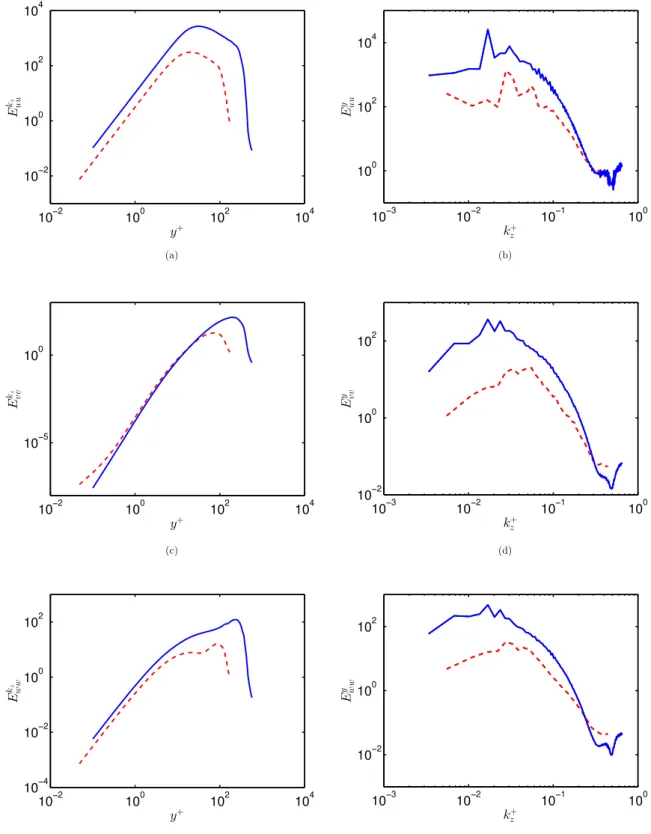
kz of order of magnitude of h. This is confirmed by the distribution of the kz-averaged premultiplied spectra k

+

zEuu (top), k+

zEvv(middle), and k

+

zEww(bottom) versus the wall-normal direction, shown in the left frames ofFig. 6, the red dashed and the solid blue lines corresponding to the optimal solutions at target time for C180 and C590, respectively. It can be observed that the wall-normal region where most of the energy is gathered is in both cases placed far from the wall, moving towards higher values of y+

when the Reynolds number is increased from 180 to 590. Moreover, the y+

-averaged premultiplied spectra plotted versus k+

z, provided in the right frames ofFig. 6, show that most of the energy is concentrated at k+_z of order 10−2, moving towards even lower values of k+

z (larger wavelengths) when going from 180 to 590. A similar trend can be observed when looking at the corre-sponding kx-premultiplied spectra (not shown), with the averaged energy peaks moving towards larger values of y+

and lower values of k+_x. Thus, the nonlinear optimal perturbations well represent the outer scale turbulent dynamics at different Re_τ, as also confirmed

by the velocity–vorticity correlation analysis that will be discussed later.

In order to investigate how the dominant streamwise wave-lengths of the optimal perturbations change when increasing Re_τ, we compare the corresponding streamwise energy density spectra (shaded contours, top frames ofFig. 4from left to right). Increasing Re_τ, not only the spectrum moves to higher values of y+

, but also appears to stretch in the wall-normal direction, showing large values for a wider range of wall-normal positions. This means that high-amplitude streamwise disturbances can be recovered not only close to the wall (where the spectrum peak is located) but also in the outer region, indicating that streaky structures are indeed recovered at larger scales. Whereas, for Re_τ

=

180, the high-amplitude zone of the spectrum is confined close to the peak value, meaning that high-amplitude streaky structures are observed mainly at a precise near-wall position. It is also worth to notice that, while for the streamwise energy spectrum the peak remains close to the wall even at Re_τ

=

590, for the spanwise and wall-normal spectra the peak moves into the outer region, where most of the vortical structures are indeed located.

Moreover, in order to analyse the streamwise coherence of the optimal perturbations and to identify the main features of streaky structures, one may investigate whether the peaks of these spectra move towards larger or smaller values of k+

x when the Reynolds number changes.Fig. 4shows that the streamwise en-ergy density peak moves to much smaller wavenumbers (larger

(a) Contours of k+ xEuu(k+x), C180. (b) Contours of k + xEuu(k+x), C590. (c) Contours of k+ xEvv(k + x), C180. (d) Contours of k + xEvv(k + x), C590. (e) Contours of k+ xEww(k + x), C180. (f) Contours of k + xEww(k + x), C590.

Fig. 4. Contours of the logarithm of the premultiplied energy density spectra in the k+

x −y

+

plane for the optimal solutions at target time (shaded contours) and the DNS (solid lines) for C180 (left) and C590 (right). The symbols X indicate the peak values of the optimal spectra. The grey zones for C180 indicate the cut off values of y+_{and k}+

x

corresponding to the half height and streamwise length of the channel.

wavelengths) for increasing Re_τ (from left to right), whereas the peak of the spanwise and wall-normal energy spectra show but a slight decrease of k+

x (the peak values, indicated by the green crosses inFig. 4are provided inTable 2for the ease of the reader). In particular, considering the streamwise energy spectra, the ratio between the two streamwise most energetic wavelengths at the two considered Reynolds numbers is close to the ratio of the two considered Re_τ themselves,

λ

+

x 590

/λ

+

x 180

≈

Reτ590

/

Reτ180 (see

Table 2). Thus, the main streamwise wavelength of the streamwise

disturbances scales with the outer unit for the two considered Reynolds numbers, although no general conclusion can be driven for other values of Re_τ. Whereas, for the wall-normal and spanwise energy spectra, the dominating

λ

+

x slightly changes with Reτ. This indicates that the main size of the wall-normal and spanwise optimal perturbations, representative of the vortical structures, changes with the inner units. A very good scaling with inner units has been also found by Hwang [38] for both the wall normal and spanwise velocity in the near-wall region. However, the nature

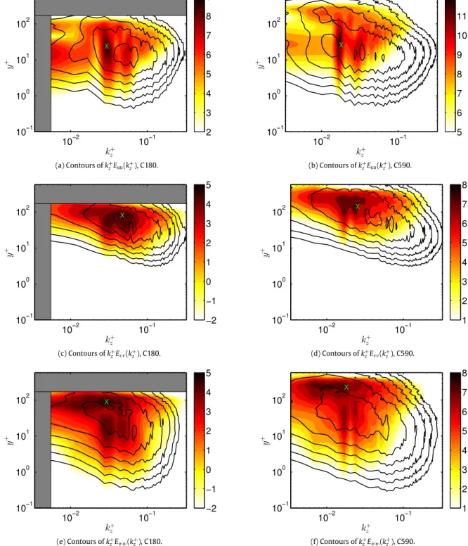
(a) Contours of k+ zEuu(k+z), C180. (b) Contours of k + zEuu(k+z), C590. (c) Contours of k+ zEvv(k + z), C180. (d) Contours of k + zEvv(k + z), C590. (e) Contours of k+ zEww(k + z), C180. (f) Contours of k + zEww(k + z), C590.

Fig. 5. Contours of the logarithm of the premultiplied energy density spectra in the k+

z −y

+

plane for the optimal solutions at target time (shaded contours) and the DNS (solid lines) for C180 (left) and C590 (right). The symbols X indicate the peak values of the optimal spectra. The grey zones for C180 indicate the cut off values of y+

and k+

z

corresponding to the half height and spanwise length of the channel.

of such a dependence would deserve a deeper analysis extended to higher Reynolds numbers. These results indicate that, for the largest considered Reynolds number, the optimal perturbation is characterized by streamwise-elongated streaks with increasing size reaching the outer scale, as well as vortical structures of smaller size.

In order to analyse the dynamics at the outer scale for the two considered Reynolds numbers, we analyse the two-point space correlation of the flow structures extracted from the DNS of tur-bulent channel flow as well as from the optimal perturbations

Table 2

Wavelength and corresponding wall-normal position of the peaks of the premul-tiplied energy density spectra shown inFigure 4.

Reτ Euu Evv Eww λ+ x 180 (C180) 757.5 757.5 757.5 λ+ x 590 (C590) 1857 928.7 619.1 y+ 180 (C180) 67.60 98.18 81.48 y+ _{590 (C590) 47.80 229.0 209.6}

Fig. 6. Premultiplied energy spectra k+

zEuu(top), k+zEvv(middle), and k

+

zEww(bottom), averaged with respect to (right) the spanwise wavenumber kzand (left) the wall-normal

direction (the superscript in the ordinates indicating the averaging direction). The red dashed and the solid blue lines correspond to the optimal solutions at target time for C180 and C590, respectively.

at target time. This technique is often used in turbulent flows to characterize the behaviour of the coherent motion, i.e. the shape and size of coherent structures. Different kinds of correlation might be used, i.e., velocity–velocity, velocity–vorticity, or conditioned correlation, as discussed by Chen et al. [34], Sillero et al. [40] and Hwang et al. [41]. Here, we employ a velocity–vorticity

correlation [34] to link the dynamics of the vortical structures (such as streamwise vortices) to the (streaky) velocity components. Following [34,41], the velocity–vorticity correlation is defined as:

Rij(yr

,

rx

,

y

,

rz)

=

⟨

u′_i(x

,

yr

,

z)

ω

′ j(x

+

rx

,

y

,

z

+

rz)

⟩

u′ i,rms

ω

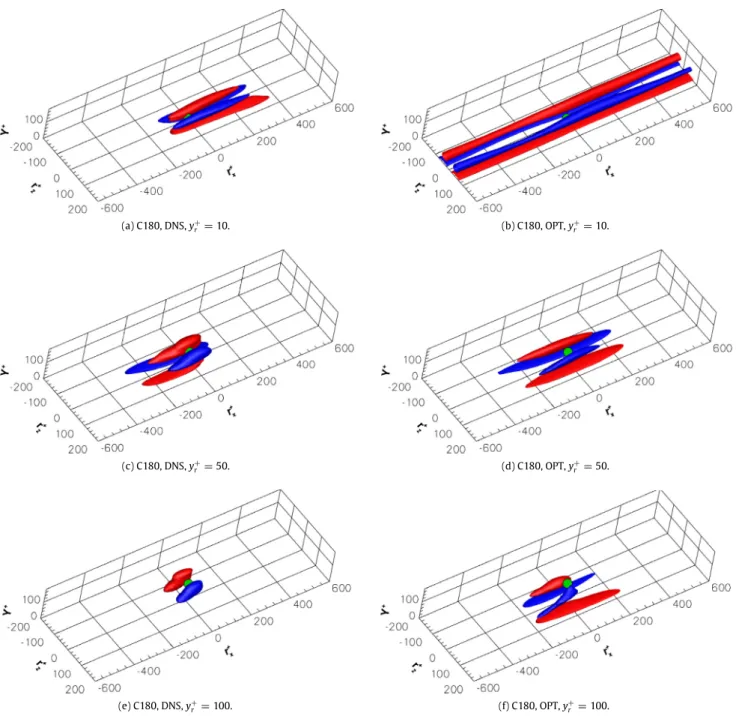
′ j,rms (3)

(a) C180, DNS, y+ r =10. (b) C180, OPT, y + r =10. (c) C180, DNS, y+ r =50. (d) C180, OPT, y + r =50. (e) C180, DNS, y+ r =100. (f) C180, OPT, y + r =100.

Fig. 7. Isosurfaces of the two-point cross-correlation coefficient (R11 =0.12) for the DNS (left) and the optimal perturbation at target time (right) for C180. Red (blue)

surfaces represent positive (negative) values. The green circles represent the reference points y+

r, with values y

+

r =10,50,100 (top to bottom). (For interpretation of the

references to colour in this figure legend, the reader is referred to the web version of this article.)

whereω′

is the vorticity perturbation; i

,

j

=

1

,

2

,

3 denote the streamwise, wall normal and spanwise components, respectively; yr is the reference wall-normal distance; rx

,

rz are the correla-tion lengths in the streamwise and spanwise direccorrela-tions and

⟨•⟩

represents the corresponding spatial average operator in the ho-mogeneous directions. In particular, the first component of this tensor, R11, provides the correlation between streamwise vortices

and streaks, helping at identifying the regions where the lift-up mechanism [9] is indeed active. For the DNS at Re_τ

=

180, as discussed also by Chen et al. [34], increasing the value of y+_r from the buffer layer to the logarithmic one, the shape of the highly-correlated structures changes, as one can observe inFig. 7(left) providing the three dimensional two-point correlation R11for the

instantaneous turbulent field at three values of y+

r

=

10

,

50

,

100. In particular, close to the wall, a quadrupole configuration (called by Chen et al. [34] a ‘‘four cigar structure’’) characterized

by elongated streaky structures is observed, indicating a strong correlation between the reference wall-normal point and the near-wall region. This shape is associated with the lift-up mechanism, as confirmed by the presence of near wall streaks and streamwise counter-rotating vortices. Increasing y+

r , the correlation becomes much weaker close to the wall, taking a dipole shape (called by Chen et al. [34] a ‘‘two blob structure’’), which suggests the presence of bulge structures linked to the head of hairpin vortices [42], frequently observed at the outer scale. The optimal perturbation at Re_τ

=

180 (right column ofFig. 7), is characterized by a very similar correlation, showing: (i) an elongated quadrupole cigar structure near the wall associated to the presence of the streaks; (ii) the dis-appearance of these elongated streaks when moving the reference point y+

r far from the wall; (iii) the onset of a bulge at y

+

r

=

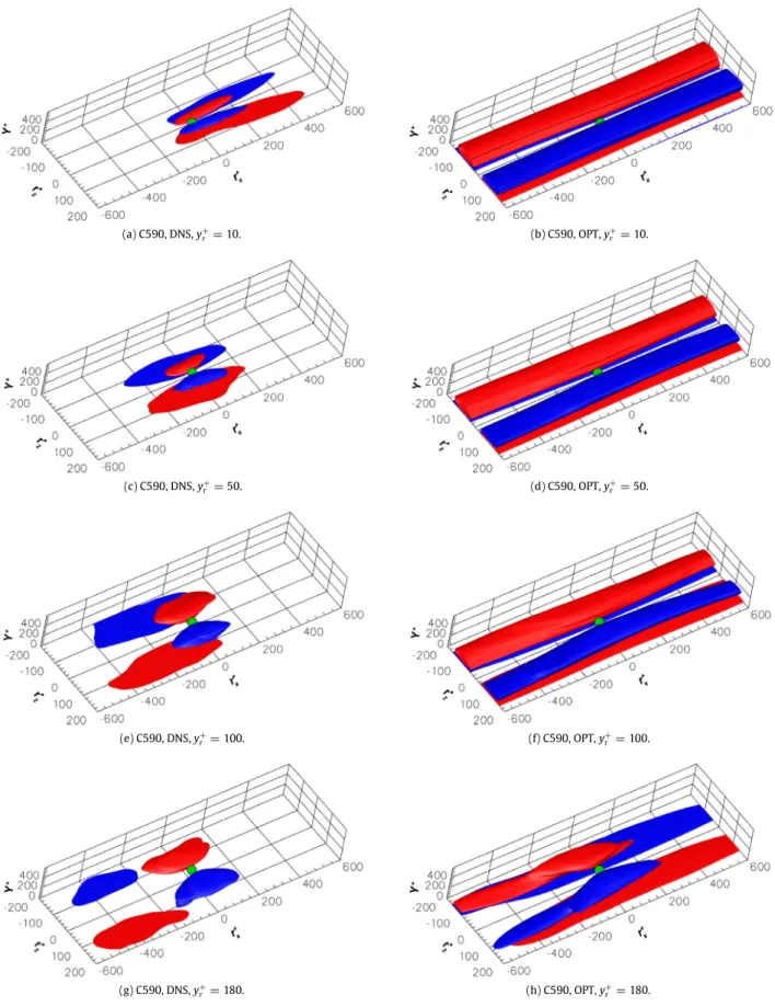
100 indicating the presence of hairpin vortices heads lifted up from the wall. One can also notice that, in the optimal perturbation at

(a) C590, DNS, y+ r =10. (b) C590, OPT, y + r =10. (c) C590, DNS, y+ r =50. (d) C590, OPT, y + r =50. (e) C590, DNS, y+ r =100. (f) C590, OPT, y + r =100. (g) C590, DNS, y+ r =180. (h) C590, OPT, y + r =180.

Fig. 8. Isosurfaces of the two-point cross-correlation coefficient (R11 =0.12) for the DNS (left) and the optimal perturbation at target time (right) for C590. Red (blue)

surfaces represent positive (negative) values. The green circles represent the reference points y+

r, with values y

+

r =10,50,100,180 (top to bottom). (For interpretation of

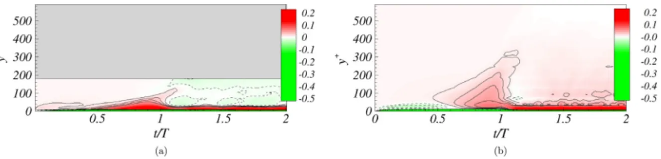
Fig. 9. Time evolution of the net local energy production, given by the difference between the production and dissipation at each y+_{for the optimal disturbance for C180 (left)} and C590 (right). Continuous and dashed lines represent respectively positive and negative values. The grey zones for C180 indicate the cut off values of y+_{corresponding} to the half size of the channel.

Re_τ

=

180, the near-wall region remains correlated with the outer one (see the two near-wall structures in the bottom right frame of

Fig. 7for y+

r

=

100). This feature is consistent with the fact that the hairpin vortices constituting the optimal perturbation provide a connection between the near-wall region and the outer one during the bursting process, as discussed by Farano et al. [15].

For the case C590, a different structure hierarchy has been observed.Fig. 8(left) provides the correlation structures extracted from the DNS for y+

r

=

10

,

50

,

100

,

180. For all of the considered values of y+_r, the quadrupole structure, indicating the presence of the lift-up mechanism, is preserved, resulting in the generation of streaky coherent structures at the wall and in the outer region. In particular, in the linear and buffer region, the structures have similar size to those observed for C180, preserving the near-wall spacing of about 100 viscous length units. Whereas, increasing y+

r , the correlation structures begin to drift in the spanwise di-rections [41], increasing their spanwise size. This larger spacing for y+

r

=

100

,

180 is present also close to the wall (see the bottom left frame ofFig. 8), indicating that the counter-rotating streamwise vortices producing the streaks extend themselves from the outer region to the wall, creating large-scale streaks [17,24] having a spanwise size of order of magnitude of h (in inner units, h+

₌

Re_τh). The absence of blob-like structures even at y+

r

=

180 suggests the weaker relevance of hairpin structures at this higher value of the Reynolds number, as it also appears by inspecting

Fig. 3. Concerning the optimal perturbation at Re_τ

=

590, the right frames ofFig. 8provide again the quadrupole structure linked with the presence of the streaks at all values of y+

r. However, the spanwise and streamwise size of the correlation structures remain large independently of y+

r, being the perturbation optimized with reference to an outer time scale.

The correlation results further confirm that, for the higher value of the Reynolds number, the optimal perturbation is mostly char-acterized by robust streaks reaching the outer scale, along with less coherent hairpin vortices. This might be linked to the fact that, unlike the case C180 [7], for larger values of Re_τ a positive (although weak) production of turbulent kinetic energy is found outside the buffer zone [25]. Such a net energy production might be associated to the lift-up mechanism, which is confined at the wall at small values of the Reynolds number and extends also at the outer scale for increasing values of Re_τ, sustaining the development of large-scale streaks. To ascertain the presence of kinetic energy production at the outer scale in the optimal perturbation, we have integrated in time the NS′ Eqs. (1)initialized with the optimal solutions, measuring the difference between production and dis-sipation terms, P(x

,

t)

= −

u′

_·

(

u′

_{· ∇}

U

)

and D(x

,

t)

=

1

/

Re

∇

u′

_:

∇

u′

, integrated along the homogeneous directions, referred to as Px,z(y

,

t) and Dx,z(y

,

t), respectively. The results are shown inFig. 9, providing the net energy production Px,z

−

Dx,zin a y+versus time plane. In both cases, for t

<

T , a positive energy production (solid contours) extends from the inner to the outer region, associated

to the energy growth of the optimal structures reaching the outer region [15]. On the other hand, for t

>

T , the two flows have different behaviours. For C590 (right), the net energy production in the outer zone is positive, which is likely due to the presence of a strong coherent lift-up mechanism acting at the outer region. Whereas, for C180 and t

>

T , (seeFig. 9(left)), the outer region is characterized by dissipation (dashed contours) associated with the breakdown of the hairpin vortices [15].

This suggests that, for the lower considered Reynolds number (C180), the energy production due to the lift-up mechanism is confined to the wall, whereas coherent hairpin vortices can reach the outer scale as a result of burst events dissipating the energy produced at the wall [15], explaining the observations of these structures at low values of Re_τ [33,39]. On the other hand, for C590, the outer scale coherent lift-up mechanism [17] generates large scale streaks, explaining the presence of the positive net energy production in the outer region. In order to confirm that this production peak is indeed linked to the presence of the lift-up mechanism, we have computed the spatial distribution of the production term P(x)

= −

u′

_v

′

_∂

U

/∂

y, which represents the wall-normal transport of the base flow shear. This term can be linked to both the lift-up [43] and the Orr mechanism [44]. However, according to Jiménez [45] and as also verified for the optimal perturbation in the case C180 [15], the linear energy growth due to the Orr mechanism is dominant for tOrr

=

t+

/

Reτ

<

0

.

15. In our case, this estimated time is much lower than the consid-ered target time (in particular, T+

/

Re_τ

=

1

.

694 for C180 and T+

_/

Re_τ

=

1

.

481 for C590). Therefore, at the target time, the main contribution to P is due to the lift-up mechanism. Fig. 10

shows the spatial distribution of P averaged in the streamwise direction for the optimal perturbations at Re_τ

=

180 (left) and 590 (right). One can observe that the lift-up mechanism is active mainly at y+

_≤

100 for C180, whereas for C590 it extends up to y+

_≈

300, corresponding to the wall-normal region at which an outer production energy peak is found in the DNS for Re_τ

=

590 (see [25]). Moreover, the lift-up mechanism appears to be active in correspondence with the large-scale streaks represented by the solid lines protruding into the outer region. This indicates that the kinetic energy production peak observed at the outer scale in several DNS for sufficiently large values of the Reynolds number is indeed due to the lift-up mechanism sustaining the large-scale streaks, which constitute (most part of) the optimal perturbation at this value of Re_τ. Whereas, for the lower values of the friction Reynolds number, optimally-amplifying perturbations are found to be mostly composed of hairpin vortices, which are not able to produce kinetic energy. The reason for this structural change with Re_τ in the optimal coherent structures has yet to be investigated in detail. However, the results presented here indicate that the existence of an outer kinetic energy production peak at sufficiently large Reynolds numbers in turbulent channel flows is indeed due to the onset of optimally growing large-scale streaks which overtake the growth of the (dissipating) hairpin vortices able to maximize the energy growth at low values of Re_τ.

Fig. 10. Lift-up production term averaged in the streamwise direction (shaded contours) and streamwise instantaneous velocity component (solid contours) in a z+₋

y+ plane for the optimal perturbations in C180 (left) and C590 (right). The grey zones for C180 indicate the cut off values of y+

corresponding to the half size of the channel.

(a) C180. (b) C180.

(c) C590. (d) C590.

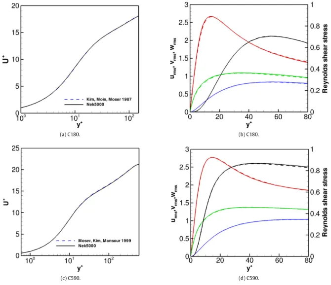
Fig. 11. Left frames: mean velocity profile U+

versus the wall-normal coordinate y+

obtained by the present DNS (solid lines) compared with literature results (dashed lines). Right frames: root mean square of u′

(red),v′ (blue),w′

(green), and Reynolds shear stress u′_v′_{(black) normalized by the wall shear velocity, versus y}+

obtained by the present DNS (solid lines) compared with results available in the literature (dashed lines). Top and bottom frames correspond to C180 and C590, respectively, the reference cases being [1] for C180 and [25] for C590.

4. Conclusions

Coherent structures are well organized motions of fluid flows with high spatial and temporal correlation. In simple turbulent shear flows, they can take the form of packets of hairpin vortices mostly placed in the outer region of the boundary layer along with streaks of different size, going from the near-wall to the outer region. Previous works, restrained to a linear approximation, have found that the latter are optimally-growing perturbations of

the turbulent mean profile at different scales (see [22]). Whereas, when taking into account nonlinear effects, the optimal pertur-bations becomes mostly composed by hairpin vortices, at least at low friction Reynolds number such as Re_τ

=

180 [15]. In this work we aim at investigating whether large-scale streaks can be considered optimally-growing perturbations of the mean veloc-ity profile in a turbulent channel flow, also in the more general nonlinear framework. Towards this end, we compare nonlinear optimal perturbations of the mean flow at two friction Reynolds

numbers, namely, Re_τ

=

180 and 590, for a target time typical of the motion at the outer scale. For the lower value of the Reynolds number, the nonlinear optimal perturbation is represented by coherent hairpin vortices originated by the breakup of the near-wall streaks, dissipating in the outer region the energy produced at the wall. Whereas, at the higher Reynolds number, the non-linear optimal perturbation is composed of more robust large-scale streaks and less coherent vortical structures. As confirmed by the turbulent kinetic energy balance, the large-scale streaks are generated by a coherent large-scale lift-up mechanism, which acts as a source term in the energy balance, inducing a positive turbulent kinetic energy production at the outer scale. The coher-ent structures induced by the lift-up mechanism as well as their dominating wavelengths are quantitatively analysed by means of two-point correlations and premultiplied kinetic energy spectra. The results of such analyses suggest that large-scale streaks are a highly energetic feature of turbulent channel flows at a sufficiently high Reynolds number, being recovered by energy optimization in both linear and nonlinear conditions. Moreover, the fact that for the higher value of Re_τ the optimally-growing perturbations are mostly characterized by large-scale streaks (instead of hairpin vortices) may be linked to the onset of a kinetic energy production peak at the outer scale at values of Re_τ between 180 and 590, as observed in the DNS by several authors [25]. In fact, between these two Reynolds numbers, we observe that the outer lift-up mechanism becomes the optimal mechanism for energy growth, leaving a clear signature in the turbulent kinetic energy budget, namely, the outer production peak observed in the literature.

Thus, in this work we have identified the physical reason for the presence of large-scale streaks at Re_τ

=

590, suggesting that they are linked to an optimal nonlinear large-scale lift-up effect. Moreover, we have linked this mechanism to the presence of a secondary peak on the kinetic energy production distribution. In future works, it would be interesting to determine whether the optimal coherent structures further change at higher values of the Reynolds number for which a more evident scale separation be-tween the size of the coherent structures populating the inner and the outer regions exists [37]. In particular, a crucial point would be to confirm (or, else, to confute) the fading of hairpin vortices in the optimal solution at higher Reynolds numbers, in order to assess, as postulated by many authors, that they are a robust coherent structure mostly for the transitional flow regime [39]. However, at the moment, extending the present analysis to higher Reynolds numbers represents a tough computational challenge due to the high CPU time required for the optimizations.

Acknowledgements

This work was granted access to HPC resources of IDRIS under allocation x20162a6362 made by GENCI (Grand Equipement Na-tional de Calcul Intensif). The authors also wish to acknowledge the computational resources of the PrInCE project (grant PONa3-00372–CUP D91D11000100007) at Politecnico di Bari.

Appendix

For validation purpose, in thisAppendixwe show the mean flow velocity U+

computed by DNS averaging the instantaneous velocity field over a long time interval (namely, about 13 time units tu_τ

/

h) and over the two homogeneous directions. The resulting velocity profile is shown in the left frames ofFig. 11(solid lines), which is compared to the mean flow computed (dashed lines) by Kim et al. [1] at C180 (top frame) and by Moser et al. [25] for C590 (bottom frame). Subtracting the computed mean flow from the instantaneous velocity field, we have obtained the perturbation

u′

, used to compute u′ u′

, which is then averaged in time and

over the two homogeneous directions. The right frames ofFig. 11

provide the root-mean-square of u′

,

v

′

,

w

′

, as well as the Reynolds shear stress u′

v

′_{, extracted from the DNS (solid lines), showing an}

excellent agreement with the same quantities computed by Kim et al. [1] and Moser et al. [25] (dashed lines) for C180 and C590, respectively.

References

[1] J. Kim, P. Moin, R. Moser, Turbulence statistics in fully developed channel flow at low Reynolds number, J. Fluid Mech. 177 (1987) 133–166.

[2] P. Luchini, Universality of the turbulent velocity profile, Phys. Rev. Lett. 118 (2017) 224501.

[3] R.L. Panton, Overview of the self-sustaining mechanisms of wall turbulence, Prog. Aerosp. Sci. 37 (2001) 341–383.

[4] S.J. Kline, W.C. Reynold, F. Schraub, P. Rundstander, The structure of turbulent boundary layer flows, J. Fluid Mech. 30 (1967) 741–773.

[5] S.B. Pope, Turbulent Flows, 2001.

[6] J.M. Hamilton, J. Kim, F. Waleffe, Regeneration mechanisms of near-wall tur-bulence structures, J. Fluid Mech. 287 (1995) 317–348.

[7] J. Jiménez, The physics of wall turbulence, Physica A 263 (1999) 252–262.

[8] F. Waleffe, On a self-sustaining process in shear flows, Phys. Fluids (1994-Present) 9 (1997) 883–900.

[9] M. Landahl, A note on an algebraic instability of inviscid parallel shear flows, J. Fluid Mech. 98 (1980) 243–251.

[10] K.M. Butler, B.F. Farrell, Optimal perturbations and streak spacing in wall-bounded turbulent shear flow, Phys. Fluids A (1989–1993) 5 (1993) 774–777.

[11] P. Luchini, Reynolds-number-independent instability of the boundary layer over a flat surface: optimal perturbations, J. Fluid Mech. 404 (2000) 289–309.

[12] C.C.T. Pringle, R. Kerswell, Using nonlinear transient growth to construct the minimal seed for shear flow turbulence, Phys. Rev. Lett. 105 (2010) 154502.

[13] S. Cherubini, P. De Palma, J.-C. Robinet, A. Bottaro, Rapid path to transition via nonlinear localized optimal perturbations in a boundary-layer flow, Phys. Rev. E 82 (2010) 066302.

[14] A. Monokrousos, A. Bottaro, L. Brandt, A. Di Vita, D.S. Henningson, Nonequilibrium thermodynamics and the optimal path to turbulence in shear flows, Phys. Rev. Lett. 106 (2011) 134502.

[15] M. Farano, S. Cherubini, J.-C. Robinet, P. De Palma, Optimal bursts in turbulent channel flow, J. Fluid Mech. 817 (2017) 35–60.

[16] Y. Hwang, C. Cossu, Self-sustained process at large scales in turbulent channel flow, Phys. Rev. Lett. 105 (2010) 044505.

[17] Y. Hwang, C. Cossu, Self-sustained processes in the logarithmic layer of turbu-lent channel flows, Phys. Fluids (1994-Present) 23 (2011) 061702.

[18] S. Rawat, C. Cossu, Y. Hwang, F. Rincon, On the self-sustained nature of large-scale motions in turbulent Couette flow, J. Fluid Mech. 782 (2015) 515–540.

[19] B. Balakumar, R. Adrian, Large-and very-large-scale motions in channel and boundary-layer flows, Philos. Trans. R. Soc. Lond. Ser. A Math. Phys. Eng. Sci. 365 (2007) 665–681.

[20] Y. Hwang, Statistical structure of self-sustaining attached eddies in turbulent channel flow, J. Fluid Mech. 767 (2015) 254–289.

[21] Y. Hwang, Y. Bengana, Self-sustaining process of minimal attached eddies in turbulent channel flow, J. Fluid Mech. 795 (2016) 708–738.

[22] G. Pujals, M. García-Villalba, C. Cossu, S. Depardon, A note on optimal transient growth in turbulent channel flows, Phys. Fluids (1994-Present) 21 (2009) 015109.

[23] C. Cossu, G. Pujals, S. Depardon, Optimal transient growth and very large–scale structures in turbulent boundary layers, J. Fluid Mech. 619 (2009) 79–94.

[24] Y. Hwang, C. Cossu, Amplification of coherent streaks in the turbulent couette flow: an input–output analysis at low Reynolds number, J. Fluid Mech. 643 (2010) 333–348.

[25] R.D. Moser, J. Kim, N.N. Mansour, Direct numerical simulation of turbulent channel flow up to reτ=590, Phys. Fluids 11 (1999) 943–945.

[26] P. Fischer, J. Lottes, S. Kerkemeir, nek5000 Web pages, 2008,http://nek5000m cs.anl.gov.

[27] M.O. Deville, P.F. Fischer, E.H. Mund, High-order Methods for Incompressible Fluid Flow, vol. 9, Cambridge University Press, 2002.

[28] C.C. Pringle, A.P. Willis, R.R. Kerswell, Minimal seeds for shear flow turbulence: using nonlinear transient growth to touch the edge of chaos, J. Fluid Mech. 702 (2012) 415–443.

[29] S. Cherubini, P. De Palma, Nonlinear optimal perturbations in a Couette flow: bursting and transition, J. Fluid Mech. 716 (2013) 251–279.

[30] Y. Duguet, A. Monokrousos, L. Brandt, D.S. Henningson, Minimal transition thresholds in plane Couette flow, Phys. Fluids (1994-Present) 25 (2013) 084103.

[31] M. Farano, S. Cherubini, J.-C. Robinet, P. De Palma, Subcritical transition scenar-ios via linear and nonlinear localized optimal perturbations in plane poiseuille flow, Fluid Dyn. Res. 48 (2016) 061409.

[32] J.C.R. Hunt, A. Wray, P. Moin, Eddies, stream, and convergence zones in turbu-lent flows, Center for Turbulence Research Report, CTR-S88, 1988.

[33] X. Wu, P. Moin, Forest of hairpins in a low-Reynolds-number zero-pressure-gradient flat-plate boundary layer, Phys. Fluids (1994-Present) 21 (2009) 091106.

[34] J. Chen, F. Hussain, J. Pei, Z.-S. She, Velocity–vorticity correlation structure in turbulent channel flow, J. Fluid Mech. 742 (2014) 291–307.

[35] R.J. Adrian, Hairpin vortex organization in wall turbulence, Phys. Fluids (1994-Present) 19 (2007) 041301.

[36] S. Toh, T. Itano, Interaction between a large-scale structure and near-wall structures in channel flow, J. Fluid Mech. 524 (2005) 249–262.

[37] A.J. Smits, B.J. McKeon, I. Marusic, High-Reynolds number wall turbulence, Annu. Rev. Fluid Mech. 43 (2011) 353–375.

[38] Y. Hwang, Mesolayer of attached eddies in turbulent channel flow, Phys. Rev. Fluids 1 (2016) 064401.

[39] T. Sayadi, C.W. Hamman, P. Moin, Direct numerical simulation of complete h-type and k-h-type transitions with implications for the dynamics of turbulent boundary layers, J. Fluid Mech. 724 (2013) 480–509.

[40]J.A. Sillero, J. Jiménez, R.D. Moser, Two-point statistics for turbulent boundary layers and channels at Reynolds numbers up toδ+_≈

2000, Phys. Fluids (1994-Present) 26 (2014) 105109.

[41]J. Hwang, J. Lee, H.J. Sung, T.A. Zaki, Inner–outer interactions of large-scale structures in turbulent channel flow, J. Fluid Mech. 790 (2016) 128–157.

[42]J. Zhou, R.J. Adrian, S. Balachandar, T. Kendall, Mechanisms for generating coherent packets of hairpin vortices in channel flow, J. Fluid Mech. 387 (1999) 353–396.

[43]L. Brandt, The lift-up effect: the linear mechanism behind transition and turbulence in shear flows, Eur. J. Mech. B Fluids 47 (2014) 80–96.

[44]W.M. Orr, The stability or instability of the steady motions of a perfect liquid and of a viscous liquid. Part II: A viscous liquid, Math. Proc. R. Ir. Acad. (1907) 69–138. JSTOR.

[45]J. Jiménez, Direct detection of linearized bursts in turbulence, Phys. Fluids 27 (2015) 065102.