HAL Id: tel-02057149
https://tel.archives-ouvertes.fr/tel-02057149
Submitted on 5 Mar 2019HAL is a multi-disciplinary open access archive for the deposit and dissemination of sci-entific research documents, whether they are pub-lished or not. The documents may come from teaching and research institutions in France or abroad, or from public or private research centers.
L’archive ouverte pluridisciplinaire HAL, est destinée au dépôt et à la diffusion de documents scientifiques de niveau recherche, publiés ou non, émanant des établissements d’enseignement et de recherche français ou étrangers, des laboratoires publics ou privés.
Numerical simulation of acoustic propagation in a
turbulent channel flow with an acoustic liner
Robin Sebastian
To cite this version:
Robin Sebastian. Numerical simulation of acoustic propagation in a turbulent channel flow with an acoustic liner. Fluids mechanics [physics.class-ph]. Université de Poitiers, 2018. English. �NNT : 2018POIT2297�. �tel-02057149�
T H E S E
Pour l’obtention du Grade deDOCTEUR DE L’UNIVERSITE DE POITIERS (Faculté des Sciences Fondamentales et Appliquées)
(Diplôme National - Arrêté du 25 mai 2016)
Ecole Doctorale : SIMMEA
Secteur de Recherche : Turbulence et Aeroacoustique
Présentée par : R O B I N S E B A S T I A N
N U M E R I C A L S I M U L AT I O N O F A C O U S T I C P R O PA G AT I O N I N A T U R B U L E N T C H A N N E L F L O W W I T H A N A C O U S T I C
L I N E R
Directeur de Thèse : Prof. Eric Lamballais
Co-directeur de Thèse : Dr. David Marx et Dr. Véronique Fortuné
Soutenue le 26 Novembre 2018 devant la Commission d’Examen
J U R Y
Laval J.-P. Directeur de recherche, CNRS, Lille Rapporteur Aurégan Y. Directeur de recherche, CNRS, Maine Rapporteur Bonnet J.-P. Directeur de recherche, CNRS, Poitiers Examinateur Perray Debain E. Professeur, Université Technologique de Compiègne Examinateur
Piot E. Chercheur, ONERA, Toulouse Examinateur
Lamballais E. Professeur, Université de Poitiers Examinateur Marx D. Chargé de recherche, CNRS, Poitiers Examinateur Fortuné V. Maître de conférences, Université de Poitiers Examinateur
A C K N O W L E D G E M E N T S
I would like to express my sincere gratitude to my thesis director Prof. Eric Lamballais and advisers Dr. David Marx and Dr. Véronique Fortuné for the continuous support of my Ph.D study and related research, for their patience, motivation, and immense knowledge. Your guidance helped me in all the time of research and writing of this thesis. I could not have imagined having a better advisor and mentors for my Ph.D study. I would like to express my special appreciation and thanks to Dr. David Marx. I would like to thank you for encouraging my research and for allowing me to explore different ideas. Your advice on both research as well as on my career have been priceless.
Besides my advisor, I would like to thank the rest of my thesis committee: Dr. Jean-Philippe Laval, Dr. Yves Aurégan, Prof. Emmanuel Perray Debain, Dr. Jean-Paul Bonnet and Dr. Estelle Piot, for accepting to be in the jury of Ph.D. defence.
My sincere thanks also goes to engineers Jean Christophe Vergez and Philippe Par-naudeau, for the IT support and access to the university computational facility SPIN Mesocenter. I would also like to thank the French Ministry of Education for the PhD fi-nancial grant, and GENCI-TGCC and GENCI-CINES for the computational grants. With-out their precious support it would not be possible to conduct this research.
I thank my fellow lab-mates for the stimulating discussions, and for all the fun we have had in the last three years.
Last but not the least, I would like to thank my parents and sister for supporting me throughout writing this thesis and my life in general.
P U B L I C AT I O N S
Some ideas and figures have appeared previously in the following publications:
Sebastian, R., Marx, D., Fortuné, V., and Lamballais, E.Numerical simulation of a com-pressible channel flow with an acoustic liner. 23rd AIAA/CEAS Aeroacoustics Confer-ence, AIAA Aviation Forum, 5-9 june 2017, Denver, Colorado. 2017.
Sebastian, R., Marx, D., Fortuné, V., and Lamballais, E.Numerical simulation of a com-pressible channel flow with impedance boundary condition. New challenges in Wall Turbulence. 2017.
Sebastian, R., Marx, D., and Fortuné, V.A scaling strategy to extract large scale motions in compressible channel flow up to Mach 3. International Journal of Heat and Fluid Flow (revision submitted)(2018).
Sebastian, R., Marx, D., and Fortuné, V. Numerical simulation of a turbulent channel flow with an acosutic liner. Journal of Sound and Vibration (under review) (2018). Sebastian, R., Marx, D., and Fortuné, V.Numerical simulation of acoustic propagation
in a turbulent spatial channel flow with acoustic liner. EFMC12. 2018.
Sebastian, R., Marx, D., Fortuné, V., and Lamballais, E.Spatial simulations of compress-ible channel flows. 2nd In(Compact) User Group Meeting, UK Turbulence Consortium. 2018.
C O N T E N T S
List of Figures
ix
List of Tables
xiv
Listings
xvi
Nomenclature
xvii
Acronyms
xix
1 introduction
1
1.1 Overview on Acoustic liners . . . 2
1.2 Overview on Wall Turbulence . . . 6
1.3 Overview on Large Eddy Simulation . . . 9
1.4 Motivations and Objectives . . . 10
1.5 Organisation of Thesis . . . 13
2 equations and simulation techniques
15
2.1 Equations . . . 152.2 Flow configuration . . . 17
2.3 Boundary conditions . . . 19
2.3.1 Periodicity . . . 19
2.3.2 Isothermal rigid wall . . . 20
2.4 Computational grid . . . 21
2.5 Numerics . . . 22
2.5.1 Spatial first-derivative . . . 22
2.5.2 Spatial second-derivative . . . 24
2.5.2.1 Modified second-derivative for DNS . . . 25
2.5.2.2 Modified second-derivative for ILES . . . 26
2.5.3 Time integration . . . 30
2.5.4 Stability Criteria . . . 31
2.6 Parallel implementation and scalability . . . 33
2.7 Validation – DNS of temporal supersonic channel flow . . . 34
3 modified finite difference scheme for implicit large eddy simulation
41
3.1 Parametric study of modified spatial 2nd-derivative Finite Difference Scheme 41 3.1.1 Channel flow at Reτ≈ 400 and M = 0.5 . . . 423.1.2 High Reτ channel flows atM = 0.5 . . . 47
3.1.3 Supersonic channel flows . . . 49
3.2 Grid requirement for wall-resolved ILES . . . 52
3.2.1 Simulation parameters . . . 52
3.2.2 Results . . . 53
3.2.2.1 Mean velocity . . . 53
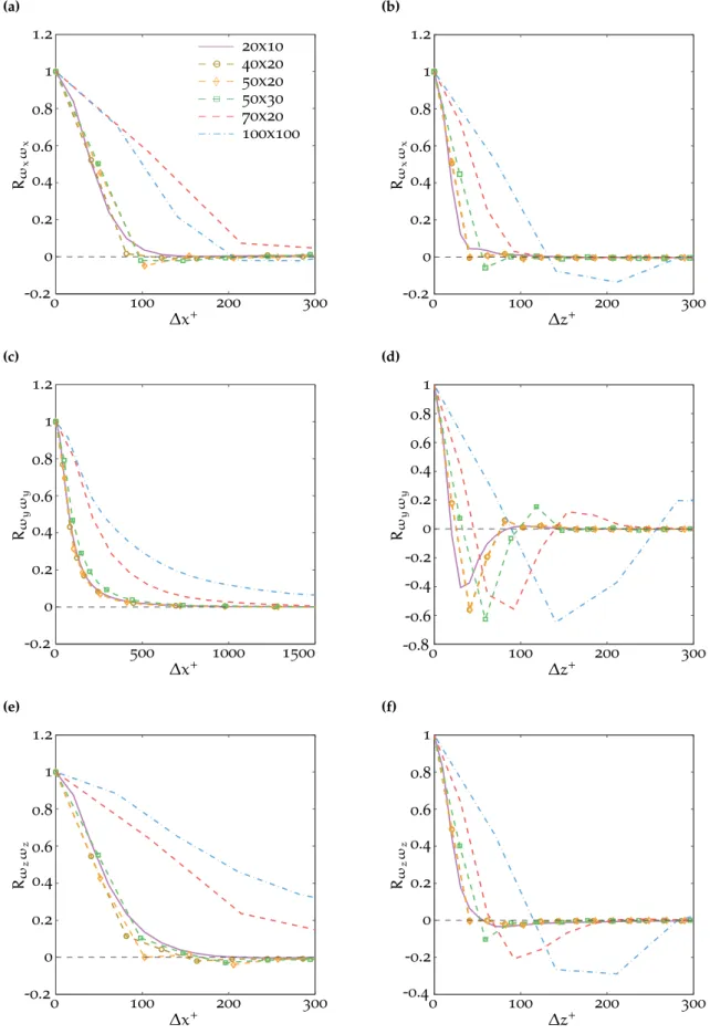
3.2.2.3 Velocity correlation and spectra . . . 56
3.2.2.4 Vorticity correlation . . . 59
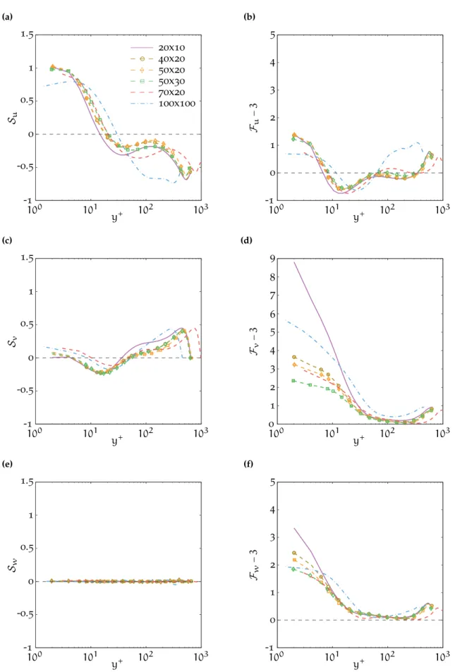
3.2.2.5 Velocity skewness and kurtosis . . . 61
3.2.3 Conclusion . . . 63
4 scaling techniques for compressible turbulent channel flow at mach number up to 3
65
4.1 Review of scaling techniques . . . 654.1.1 Incompressible transformation . . . 65
4.1.2 Compressibility effects . . . 66
4.1.3 Van Driest transformation . . . 67
4.1.4 Semi-local transformation . . . 69 4.1.5 Trettel’s transformation . . . 70 4.2 Numerical test . . . 71 4.2.1 Simulation parameters . . . 72 4.2.2 Results . . . 73 4.2.2.1 Mean velocity . . . 74
4.2.2.2 Rms profiles of velocity and vorticity . . . 74
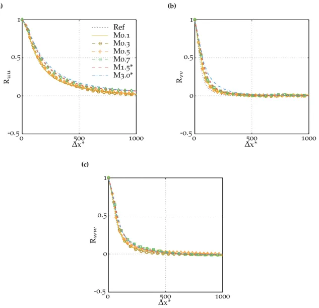
4.2.2.3 Velcity correlation . . . 78
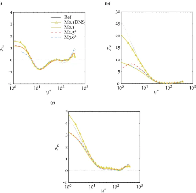
4.2.2.4 Velocity skewness and kurtosis . . . 80
4.3 Conclusion . . . 82
5 inner-outer layer scales-interaction
83
5.1 Overview on large-scale structures in wall-bounded turbulent flow . . . 835.2 Grid requirement . . . 85
5.3 Simulation at high Reynolds & Mach number . . . 87
5.3.1 Validation of the simulations . . . 87
5.3.2 Evidence of Large Scale Structures and their effect on near-wall scales 89 5.3.3 Procedure to extract large-scale structures . . . 93
5.3.4 Organisation of large-scale structures . . . 96
5.3.5 Quantification of large-scale influence . . . 102
5.4 Conclusion . . . 108
6 temporal simulation of channel flow with acoustic liner
109
6.1 Boundary condition - Impedance wall . . . 1096.1.1 Validation . . . 111
6.2 Grid requirement for channel flow with acoustic liner . . . 112
6.3 Flow statistics . . . 115
6.3.1 Effect of the liner resistance R . . . 116
6.3.2 Effect of the resonance frequency ωres . . . 117
6.3.3 Effect of the flow Mach numberM . . . 119
6.4 Existence of a wave along the acoustic liner . . . 120
6.5 Drag . . . 126
6.6 Linear stability analysis . . . 128
6.6.1 Instability due to impedance boundary . . . 128
6.6.2 Comparison with the numerical simulations . . . 131
6.7 Conclusion . . . 133
7 spatial simulation of channel flow and sound attenuation
135
7.1 Boundary conditions . . . 1357.1.1 Subsonic inflow boundary condition . . . 135
7.1.1.1 Based on Local One Dimensional Inviscid (LODI) relations 136 7.1.1.2 Based on Navier-Stokes equations . . . 137
7.1.1.3 Non-reflecting characteristics boundary condition . . . 137
7.1.2 Subsonic outflow boundary condition . . . 138
7.1.2.1 Sponge zone . . . 139
7.2 Wave extraction using global minimization . . . 141
7.3 Validation . . . 145
7.3.1 Poiseuille flow . . . 145
7.3.1.1 Flow configuration . . . 145
7.3.1.2 Results . . . 147
7.3.2 Poiseuille flow with acoustic wave . . . 148
7.3.2.1 Multiple plane acoustic waves . . . 150
7.3.2.2 Plane and transverse acoustic waves . . . 152
7.4 Spatial turbulent channel flow . . . 154
7.4.1 Turbulent inflow . . . 154
7.4.2 Turbulent flow statistics . . . 155
7.4.2.1 Simulation set-up . . . 155
7.4.2.2 Results . . . 156
7.4.3 Interaction between sound and turbulence . . . 161
7.4.3.1 Simulation setup . . . 161
7.4.3.2 Results . . . 163
7.5 Conclusion . . . 167
8 simulation of flow tube with acoustic liner
169
8.1 Simulation setup . . . 1708.2 Flow statistics . . . 172
8.3 Instability over the acoustic liner . . . 176
8.4 Turbulence-liner-acoustic interaction . . . 177
8.5 Effect on sound attenuation . . . 179
8.6 Conclusion . . . 182
9 conclusion and perspectives
183
9.1 Future works . . . 184Appendix
a brief history of code “compact3d” and coefficients for compact schemes189
a.1 History of Compact3D . . . 189a.2 Coefficient of compact schemes . . . 190
b grid stretching
193
b.1 Wall-normal grid . . . 193b.1.1 Tanh stretching . . . 193
b.1.2 Incompact stretching . . . 194
b.2 Stream-wise grid . . . 194
c comparison between dns and iles
197
e linearised 2d navier-stokes equations and boundary
con-ditions
203
f target solution for sponge zone
207
bibliography
209
L I S T O F F I G U R E S
1 Introduction
Figure 1.1 Illustration of engine noise treatment . . . 2
Figure 1.2 Schematic of grazing flow . . . 3
Figure 1.3 Regions of TBL . . . 7
Figure 1.4 Illustration of DNS, LES and RANS . . . 9
Figure 1.5 Objectives of the thesis . . . 11
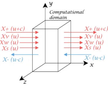
2 Equations and Simulation techniques Figure 2.1 Flow configuration for the temporal channel flow simulation . . . 17
Figure 2.2 Characteristics waves entering and leaving the computational do-main for a subsonic flow . . . 20
Figure 2.3 Illustration of wall boundary treatment . . . 20
Figure 2.4 Modified wave-numbers for spatial first-derivative . . . 23
Figure 2.5 Spatial discretisation for first-derivative in non-periodic boundary 24 Figure 2.6 Modified wave-numbers for spatial second-derivative . . . 24
Figure 2.7 Modified wave-numbers of spatial second-derivative scheme used for DNS . . . 26
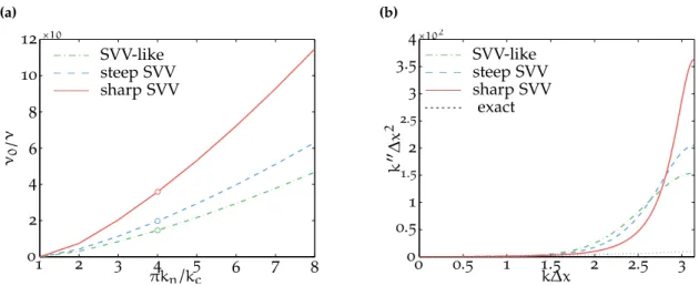
Figure 2.8 Shape of SVV kernel . . . 28
Figure 2.9 Modified wave-numbers of spatial second-derivative kernels used for ILES . . . 28
Figure 2.10 Spatial discretisation for the second-derivative in non-periodic boundary . . . 30
Figure 2.11 Constraint on explicit time stepping due to RebandM . . . 32
Figure 2.12 Time constraint due to CFL and Fourier constraint with different mesh size at the wall . . . 33
Figure 2.13 2D pencil domain decomposition using 2DECOMP library . . . 33
Figure 2.14 Scalability curves for Compact3D . . . 34
Figure 2.15 Comparison of mean velocity profile . . . 36
Figure 2.16 Comparison of rms velocity profiles . . . 36
Figure 2.17 Comparison of mean profile of scalar quantities . . . 37
Figure 2.18 Comparison of rms profile of scalar quantities . . . 38
Figure 2.19 Comparison of stress profiles . . . 38
Figure 2.20 Comparison of stream-wise and span-wise correlations . . . 39
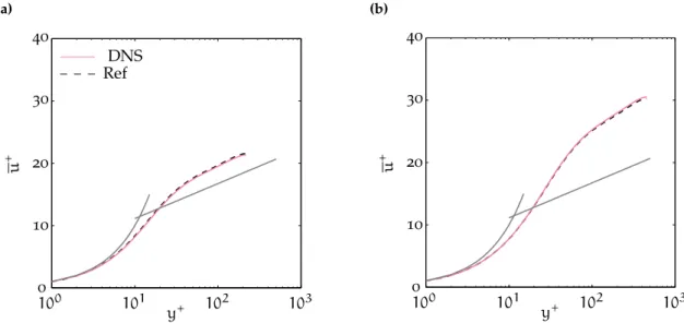
3 Modified Finite Difference scheme for Implicit Large Eddy Simulation Figure 3.1 Comparison of mean, rms velocity profiles and spectra from ILES of channel flow with fine grid at Reτ≈ 400 and M = 0.5 . . . 44
Figure 3.2 Comparison of mean and rms velocity profiles from ILES of
chan-nel flow with coarse grid at Reτ≈ 400 and M = 0.5 . . . 45
Figure 3.3 Comparison of spectra from ILES of channel flow with coarse grid at Reτ≈ 400 and M = 0.5 . . . 46
Figure 3.4 Comparison of mean and rms velocity profiles for ILES of channel flow for Reτ= 640 and 1000 at M = 0.5 . . . 48
Figure 3.5 Comparison of mean and rms velocity profiles for ILES of channel flow atM = 1.5 and Reb= 3000 . . . 50
Figure 3.6 Comparison of mean and rms velocity profiles for ILES of channel flow atM = 3 and Reb= 4880 . . . 50
Figure 3.7 Comparison of mean and rms velocity profile for analysing the grid requirement for wall-resolved ILES . . . 54
Figure 3.8 Comparison of Reynolds stress profiles for analysing the grid re-quirement for wall-resolved ILES . . . 55
Figure 3.9 Comparison of√ω′2 profiles for analysing the grid requirement for wall-resolved ILES . . . 55
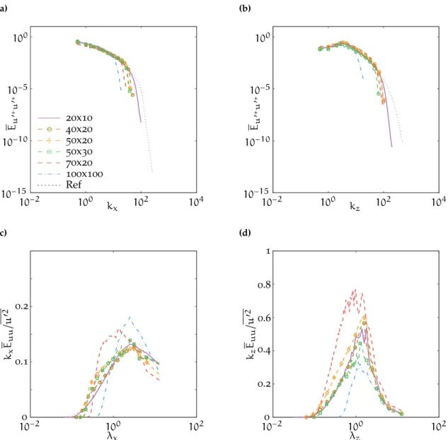
Figure 3.10 Comparison of velocity correlation in stream-wise and span-wise direction at y+ = 10 for analysing the grid requirement for wall-resolved ILES . . . 57
Figure 3.11 Comparison of stream-wise velocity spectra at y= 0.5H for analysing the grid requirement for wall-resolved ILES . . . 58
Figure 3.12 Comparison of ω correlation in stream-wise and span-wise direc-tion at y+= 10 for analysing the grid resolution for wall-resolved ILES . . . 60
Figure 3.13 Comparison of skewness and kurtosis of velocity components for analysing the grid requirement for wall-resolved ILES . . . 62
4 Scaling techniques for compressible turbulent channel flow at Mach num-ber up to 3 Figure 4.1 Mean velocity profiles for incompressible and compressible chan-nel with cold walls . . . 69
Figure 4.2 Local friction length scale as a function of wall-distance . . . 70
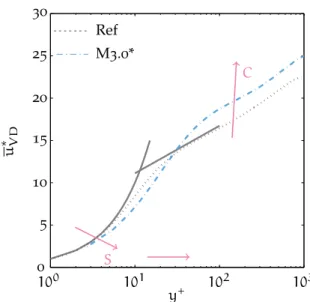
Figure 4.3 Raw and transformed mean velocity profiles . . . 74
Figure 4.4 Raw and transformed rms velocity profiles . . . 75
Figure 4.5 Rms velocity profiles for showing Reynolds number effect . . . 76
Figure 4.6 Raw and transformed rms vorticity profiles . . . 77
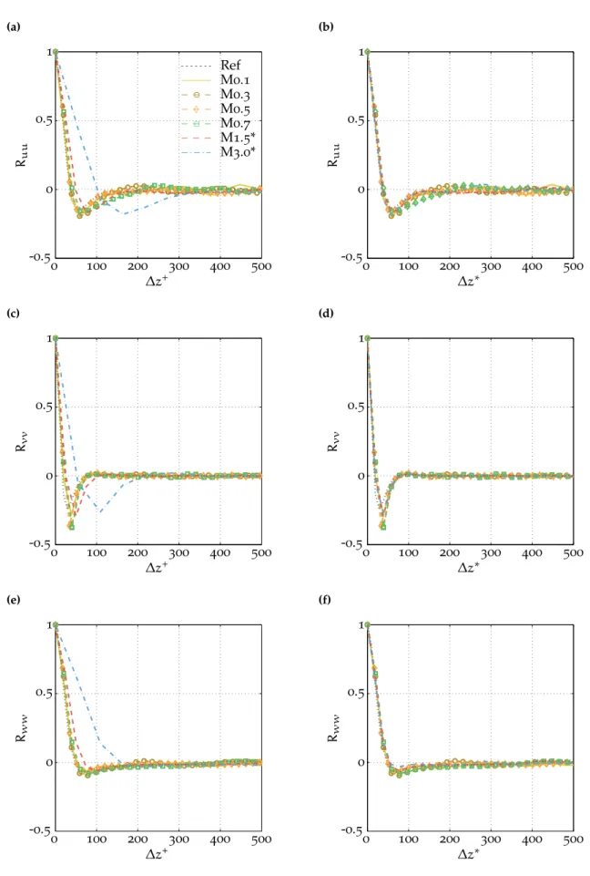
Figure 4.7 Raw and transformed near-wall span-wise correlation . . . 78
Figure 4.8 Transformed near-wall stream-wise correlation . . . 79
Figure 4.9 Velocity skewness profiles . . . 80
Figure 4.10 Velocity flatness profiles . . . 81
5 Inner-outer layer scales-interaction Figure 5.1 2D pre-multiplied stream-wise velocity spectra at y+≈ 15 . . . 86
Figure 5.3 Mean and rms of stream-wise velocity profiles . . . 88
Figure 5.4 Instantaneous visualisation of u′∗on the wall parallel plane close to the wall . . . 89
Figure 5.5 Pre-multiplied spectra of stream-wise velocity and qualitative rep-resentation of scales-interaction in the inner-outer region . . . 90
Figure 5.6 Tilting angle of the large-scale structures . . . 91
Figure 5.7 Decoupling procedure for quantifying inner-outer scales interaction 92 Figure 5.8 Amplitude modulation covariance map . . . 93
Figure 5.9 Rms of the small- and large-scale velocity fluctuation . . . 95
Figure 5.10 Example of feature extraction for large-scale structures . . . 96
Figure 5.11 Conditionally averaged LMLSS in the y− z plane . . . 97
Figure 5.12 Example of detected large-scale structures after different thresh-olding criteria . . . 99
Figure 5.13 Conditionally averaged 3D large-scale structure . . . 100
Figure 5.14 Comparison of large-scale footprint at differentM with detection based on conventional wall-units . . . 101
Figure 5.15 Comparison of large-scale footprint at differentM with detection based on semi-local units . . . 101
Figure 5.16 Organisation of large-scale structures . . . 102
Figure 5.17 Conditional statistic for the high- and low-momentum large-scale structures . . . 106
Figure 5.18 Conditional average of rms of stream-wise velocity for the high-and low-momentum large-scale structures . . . 107
Figure 5.19 Conditional average of rms of stream-wise velocity for the high-and low-momentum large-scale structures for Re∗τ= 590 and 640 . 107 6 Temporal simulation of channel flow with acoustic liner Figure 6.1 Validation curves for impedance boundary condition . . . 111
Figure 6.2 Grid convergence for impedance wall test cases . . . 113
Figure 6.3 Comparison of channel flow simulation with Scalo et al. (2015)[240] 114 Figure 6.4 Results for varying liner resistance . . . 117
Figure 6.5 Change in drag as a function of liner resistance . . . 117
Figure 6.6 Mean velocity profile for varying resonance frequency of the liner 118 Figure 6.7 Turbulent statistics for varying liner resonance frequency . . . 119
Figure 6.8 Change in drag as a function ofM number . . . 120
Figure 6.9 Velocity spectra for varying liner resonance frequency . . . 121
Figure 6.10 Instantaneous visualization of turbulent structures for channel flow with acoustic liner . . . 123
Figure 6.11 Slice of instantaneous flow field for varying liner resonance fre-quency . . . 124
Figure 6.12 Amplitude of wave along the liner . . . 125
Figure 6.13 Phase averaged drag . . . 126
Figure 6.14 Phase averaged Reynolds stress . . . 127
Figure 6.15 Complex phase speed spectrum for parabolic base flow . . . 129
Figure 6.16 Complex phase speed spectrum with MSD wall tuned to desta-bilise A-branch mode . . . 130
Figure 6.17 Eigenfunction for parabolic and steeper base flow with bottom
MSD wall . . . 131
Figure 6.18 Comparison between simulation and temporal linear stability anal-ysis for test-case AC02 . . . 132
Figure 6.19 Comparison of eigenfunction from simulation and linear stability analysis . . . 133
7 Spatial simulation of channel flow and sound attenuation Figure 7.1 Sponge layer for a spatial channel flow simulation . . . 140
Figure 7.2 Up-stream and down-stream travelling acoustic waves and the measurement configuration for the TMM . . . 141
Figure 7.3 Comparison of raw and span-wise averaged signal . . . 143
Figure 7.4 Example of transverse acoustic modes . . . 144
Figure 7.5 Flow configuration for Poiseuille flow validation . . . 146
Figure 7.6 Time evolution of inlet and outlet mass flow rate . . . 147
Figure 7.7 Mass flow rate and percentage change in pressure and tempera-ture in stream-wise direction . . . 148
Figure 7.8 Flow field for the low Reynolnds number poiseuille flow . . . 149
Figure 7.9 Comparison of simulation results with analytical solution . . . 150
Figure 7.10 Perturbation field with two plane waves . . . 151
Figure 7.11 Comparison of wave profiles from simulation and modal analysis 152 Figure 7.12 Instantaneous acoustic pressure field with plane and transverse wave . . . 153
Figure 7.13 Comparison of transverse wave profile from simulation and modal analysis . . . 153
Figure 7.14 Flow configuration for turbulent spatial channel flow simulation . 155 Figure 7.15 Mean flow field of turbulent channel flow . . . 157
Figure 7.16 Stream-wise distribution of mean flow variables . . . 158
Figure 7.17 Evolution of mean pressure and temperature . . . 159
Figure 7.18 Profiles of mean stream-wise velocity and temperature . . . 159
Figure 7.19 Comparison of Reynolds stresses profiles . . . 160
Figure 7.20 Comparison of rms profiles of thermodynamic quantities . . . 161
Figure 7.21 Simulation setup to study sound attenuation in a turbulent chan-nel flow . . . 162
Figure 7.22 Schematic of acoustic and turbulent boundary layers . . . 162
Figure 7.23 Instantaneous pressure perturbation field in turbulent channel with multiple plane waves . . . 163
Figure 7.24 Frequency spectra of wall-pressure . . . 164
Figure 7.25 Comparison of down-stream travelling acoustic wave profiles . . . 165
Figure 7.26 Comparison of wave profiles from simulation and modal analysis 166 Figure 7.27 Damping coefficient for the down-stream and up-stream travel-ling waves in a turbulent channel flow . . . 166
8 Simulation of flow tube with acoustic liner Figure 8.1 Configuration for flow tube with acoustic liner . . . 169
Figure 8.2 Instantaneous flow visualisation at bottom wall of the flow tube with lined section . . . 171 Figure 8.3 Contours of mean spatial flow-field for the flow tube with lined
section . . . 172 Figure 8.4 Evolution of mean velocity over the lined surface . . . 173 Figure 8.5 Stream-wise distribution of mean flow variables . . . 173 Figure 8.6 Evolution of mean pressure and temperature in the flow tube
with acoustic liner . . . 174 Figure 8.7 Comparison of Reynolds stress profiles . . . 175 Figure 8.8 Instantaneous wall-normal velocity on the impedance surface . . . 176 Figure 8.9 Spatial and temporal spectra over the acoustic liner . . . 176 Figure 8.10 Eigen function over acoustic liner . . . 177 Figure 8.11 Linear Stability Analysis (LSA) of experiment of Marx et al. (2010)[181]
(liner corresponding to test-case AC01) . . . 178 Figure 8.12 Turbulence-acoustic interaction for experiment of Marx et al. (2010)[181]178 Figure 8.13 LSAof simulation with liner corresponding to test-case AC02 . . . 179
Figure 8.14 Turbulence-acoustic interaction for simulation test-case AC02 . . . 179 Figure 8.15 Pressure signal and SPL on the top wall . . . 180 Figure 8.16 Stability analysis for varying resistance of the liner . . . 181 Figure 8.17 Comparison of complex wave-number over liner against the modal
analysis . . . 181 Figure 8.18 Sound attenuation in the flow-tube with liner . . . 182
C Comparison between DNS and ILES
Figure C.1 Comparison of velocity spectra obtained from different simula-tion techniques for channel flow at Reb= 3000 and M = 1.5 . . . . 198 Figure C.2 Comparison of mean velocity profiles . . . 199 Figure C.3 Comparison of rms velocity profiles . . . 200 Figure C.4 Comparison of Reynolds stress profiles . . . 200
D Compressible relationship
Figure D.1 Evolution of density and viscosity ratio as the function of M number . . . 201 Figure D.2 Evolution of ρwuτas the function ofM number . . . 202 F Target solution for sponge zone
L I S T O F TA B L E S
2 Equations and Simulation techniques
Table 2.1 Spatial discretisation for first-derivative . . . 23 Table 2.2 Spatial discretisation for second-derivative . . . 29 Table 2.3 Parameters of validation test-case for DNS of supersonic channel
flows . . . 35 Table 2.4 Validation results . . . 35
3 Modified Finite Difference scheme for Implicit Large Eddy Simulation Table 3.1 Computational grids used for the parametric study of modified
spatial 2nd-derivative FDS at Reτ≈ 400 and M = 0.5 . . . 42 Table 3.2 SVV kernels used for the parametric study of modified spatial
2nd-derivative FDS for ILES of channel flow at Re
τ ≈ 400 and M = 0.5 . . . 43 Table 3.3 Mean flow variables and errors in their prediction with different
SVV kernels for ILES of channel flow at Reτ≈ 400 at M = 0.5 . . . 43 Table 3.4 Simulation parameters and results for the parametric study of
modified spatial 2nd-derivative FDS for ILES of high Reτ channel flows . . . 48 Table 3.5 Computational grids used for the parametric study of modified
spatial 2nd-derivative FDS for ILES of supersonic channel flows . . 49 Table 3.6 Mean flow variables and their errors with different SVV kernels
for ILES of supersonic channel flows . . . 51 Table 3.7 Test-cases for analysing grid requirement for ILES of channel flows 53
4 Scaling techniques for compressible turbulent channel flow at Mach num-ber up to 3
Table 4.1 Simulation test-cases for analysing the scaling techniques . . . 73 Table 4.2 Mean flow variables for simulation test-cases for analysing
scal-ing techniques . . . 73
5 Inner-outer layer scales-interaction
Table 5.1 Simulation test-cases for studying inner-outer scales interaction at differentM numbers . . . 87 Table 5.2 Area occupied by the large-scale structures . . . 103 Table 5.3 Change in drag due to the large-scale structures . . . 104 Table 5.4 Contribution to skin-friction from the large-scale structures . . . . 104
6 Temporal simulation of channel flow with acoustic liner
Table 6.1 Grid convergence analysis with impedance boundary condition . 112 Table 6.2 Simulation test-cases with impedance boundary condition . . . 115 Table 6.3 Characteristics of the wave along the liner . . . 122 Table 6.4 Comparison between simulation and linear stability analysis . . . 132
7 Spatial simulation of channel flow and sound attenuation
Table 7.1 Comparison of wave properties computed from simulation and modal analysis for multiple plane acoustic waves . . . 152 Table 7.2 Comparison of wave properties computed from simulation and
modal analysis for plane and transverse acoustic waves . . . 154 Table 7.3 Simulation parameters to study wave attenuation in turbulent
channel flow . . . 163 Table 7.4 Details of signal used for post-processing . . . 164 Table 7.5 Properties of acoustic waves in turbulent channel flow . . . 167
A Brief history of code “Compact3D” and coefficients for compact schemes Table A.1 Compact schemes for spatial first-derivative . . . 190 Table A.2 Compact schemes for spatial second-derivative . . . 191
C Comparison between DNS and ILES
Table C.1 Computational grids for testing DNS and ILES . . . 197 Table C.2 Computational grid for comparing the benchmark channel flow
L I S T I N G S
B Grid stretching
Listing 1 Wall-normal grid stretching . . . 193 Listing 2 Stream-wise grid stretching . . . 194
N O M E N C L AT U R E
Physical quantities
η Kolmogorov scale
γ Ratio of specific heats µ Dynamic fluid viscosity
ω Angular frequency ρ Fluid density τ Stress ξ Damping ratio c Speed of sound cf Drag coefficient
cp Adiabatic specific heat
H Channel half-height h Enthalpy K Stiffness Kt Thermal conductivity lν Viscous length-scale M Mass p Pressure q Heal flux R Resistance ruv Reynolds stress s Entropy T Temperature t Time u; u1 Stream-wise velocity uτ Friction velocity v; u2 Wall-normal velocity w; u3 Span-wise velocity x; x1 Stream-wise coordinate y; x2 Wall-normal coordinate z; x3 Span-wise coordinate Non-dimensional numbers κ von Kármán constant M Mach number Bq Heat flux Pr Prandtl number Re Reynolds number C Log-law intercept
Numerics
α; β; a; b; c; d FDS coefficients ν Spectral viscosity
ν0 Spectral viscosity at cut-off
σi stability footprint on imaginary
axis
σr stability footprint on real axis
k Spatial wave-number
k′ Modified wave-number for 1th spatial derivative
k′′ Modified wave-number for 2nd spatial derivative
kc Spatial cut-off wave-number
kη Wave-number for Kolmogorov
scale
Nfac; c1 Parameters for SVV kernel shape
Simulation parameters ∆x,y,z,t Discretisation
Lx,y,z Domain length
Nx,y,z Number of grid points
Other
F Flux vector
F Flatness
S Skewness
A; <A> Mean of quantity A A′ Fluctuation of quantity A q Solution vector √ A′2 rms of quantity A F Forcing term X±; Y±; Z± Acoustic waves Xs; Ys; Zs Entropy waves Xv,w; Yu,w; Zu,v Vorticity waves Subscripts
Ab Bulk quantity A
Ac Value of quantity A at centre of
the channel
At Turbulent quantity of A
Aw Value of quantity A at the wall
Aflow Quantity A of the flow Ares Quantity A of the resonance
Awave Quantity A of the wave
Superscripts
˜A Dimensional quantity A
A∗ Quantity A after compressible transformation
A+ Quantity A scaled with viscous scales
A C R O N Y M S
2DOF Two Degree Of Freedom BPF Blade Passing Frequency CAA Computational Aero Acoustics CFD Computational Fluid Dynamics CFL Courant–Friedrichs–Lewy DGM Discontinuous Galerkin Method DNS Direct Numerical Simulation FDS Finite Difference Scheme HMLSS High Momentum Large Scale
Structure
HPC High Performance Computation IBC Impedance Boundary Condition IBM Immersed Boundary Method ILES Implicit Large Eddy Simulation LEE Linearised Euler Equations LES Large Eddy Simulation
LODI Local One Dimensional Inviscid LMLSS Low Momentum Large Scale
Structure
LSA Linear Stability Analysis LSM Large Scale Motion LSM Least Square Method MMM Mode Matching Method MPI Message Passing Interface MSD Mass-Spring-Damper NSE Navier-Stokes Equations
RANS Reynolds Averaged Navier Stokes SDOF Single Degree Of Freedom
SFM Straight Forward Method SGS Sub-Grid Scale
SNR Sound to Noise Ratio SPL Sound Pressure Level SVV Spectral Vanishing Viscosity SWR Standing Wave Ratio
TBL Turbulent Boundary Layer TMM Two Microphone Method TPM Two Port Matrix
1
I N T R O D U C T I O NAircraft and engine manufacturers are always under the continuous pressure of growing demand for quieter aircraft. This is due to the increasing quality of life and due to the necessity to compensate air traffic growth and the encroachment of neighbouring com-munities for larger airport infrastructures. Air traffic is increasing because of the time efficiency of aircraft, and it is speculated to double in the next 20 years. But at the same time aircrafts are noisy and the well-known issues associated with elevated aircraft noise level includes stress, sleep depreciation and hypertension among others. Governments and other related institutions are taking necessary actions to control the noise emission and protect people. Major source of aircraft noise can be broadly classified into (a) engine, (b) airframe and (c) mechanical vibrations. The growth in the theoretical description of many aeroacoustic mechanisms in the past sixty years has led to a progressive reduction of aircraft noise.
Engine noise is a major contributor to the aircraft noise. The first generation of aircrafts in 1960s were very noisy, which led to the introduction of high by-pass ratio turbofan engines and effective nacelle acoustic treatment. These type of engines not only reduced the sound level by 25-30 dB, but they were also very fuel efficient. This makes turbofan engines the only choice for commercial aircrafts. However, since the 1980s the noise reduction trend has not been so significant. Therefore, any further noise reduction is very difficult to be achieved without affecting the aircraft operating cost. Due to the entry of ultra high-bypass ratio turbofans into service and novel noise control devices on modern civil aircraft, the engine noise is expected to be comparable and even lower than the airframe noise generated by the high-lift devices and by the undercarriage. A great deal of interest have been devoted during the last years to the rediscovery and improvement of analytical models for both airframe and engine noise prediction using multi-disciplinary/multi-objective optimisation processes which relies on fast numerical methods[7,8,170,171].
A turbofan engine produces both tonal and broadband noises. Tonal noise is generated due to the fan, and the broadband noise is due to the turbulence. Various technologies have been developed to reduce the engine noise, such as scarf inlet, forward swept fans, trailing-edge blowing, among others acoustic treatment. Acoustic liners are key technol-ogy to absorb sound in ducts such as turbofan engines, and it is the passive method for noise reduction. Acoustic liner is a sandwich panel and work as a group of Helmholtz resonators. A single degree of freedom liner panel will include the perforated face-sheet, honeycomb structure and the solid back-plate. Some liners have multiple layers of hon-eycomb and perforated face-sheet for multiple degrees of freedom. In many practical applications they are subjected to high-speed flows and turbulence. In turbofan engines, liners are usually applied on the internal walls of the engine nacelle to absorb the radi-ated acoustic energy (seefigure 1.1for an example of acoustic liner.) Many studies have been devoted to understand the behaviour of acoustic liner, owing to the importance of
Acoustic liner
Figure 1.1: Illustration of engine noise treatment.
noise reduction. In the past, most of the research was done with the help of experimental techniques. Experimental techniques have several advantages, but the major drawback is the intrusive measurement of the flow. This indeed limits access to the major part of the flow, where one might find interesting physics. On the other hand numerical sim-ulation gives access to every point in space, but the major setback is the truncation of the computational domain and high computational cost. With the recent developments in the computer technology, High Performance Computing (HPC) has entered the reality of petascale computing. Currently,HPChas deep consequences for scientific research as it open doors for solving complex turbulence problems, which were once considered im-possible. The major objective of this Ph.D. thesis is to study how acoustic liners affect the turbulent flow and noise attenuation with the help of numerical simulations. This is an attempt to study the interaction within a complex flow physics, therefore this topic of-fers wide range of possibility for research. The thesis was conceived as a 6 step approach, therefore before presenting the motivations and the multiple objectives (in Section 1.4) a brief introduction on acoustic liners, wall-turbulence and the numerical simulation is given inSections 1.1– 1.3. Finally, the organisation of the thesis is presented inSection 1.5.
1.1 overview on acoustic liners
Acoustic liner covers most of the available surface in turbofan engines depending on the installation of other engine systems. The typical acoustic liners are locally reacting and the acoustic impedance of the liner will depend on properties of the lining, grazing flow and frequency of the sound. In the future the bypass ratio of the turbofan engine will
in-crease and the inlet length will not be scaled with the same factor. Since the performance of the liner is limited to its length, these changes will make liners less effective. Different methods of optimisation can focus on the variations in the depth of the honeycomb core, core-cell dimensions and number of layers. However from the engineering point of view, manufacturers should also keep in mind that the liner will increase the overall engine weight.
Since 1970’s acoustic liner with adjustable impedance that has potential application in the active control of duct noise and unstable flow in turbo-machines has received some attention[62,305]. It is well known that the grazing flow changes the acoustic impedance of the liner, thereby affecting the noise attenuation in the duct. A better understand-ing of this so called grazunderstand-ing flow effect is necessary for the design of efficient acoustic liners[102,148,204]. During the past decades, considerable research has been carried out to understand the effect of grazing flow on the acoustic impedance of the liner[138]. The acoustic resistance of perforated face-sheet linearly increases and the acoustic reactance slightly decreases with increasing grazing flow velocity[57,96,102,138,221]. The visualisation and the measurements of the flow details in the vicinity of an orifice reveal that vortices are generated from leading edge of the orifice under the acoustic excitation and con-vected down-stream by the mean grazing flow[208,295]. The vortical and acoustic flow at an orifice in the presence of grazing flow interacts strongly, and this leads to the change of the orifice acoustic impedance. Several investigations have been concentrated on
de-Grazing flow
Perforated facesheet
Solid backplate
Honeycomb core
Figure 1.2: Schematic of grazing flow.
scribing how sound energy is dissipated in the near-field of the orifice and theoretical models have been developed[108,116,143,236,288]. Although several models has been pro-posed with different assumption and in order to make the model flexible the problem has been generally over simplified. Theoretical modelling of the acoustic behaviour of perforates subjected to grazing flow is mainly dependent on the experimental data.
Mea-surement of the impedance of perforated plates is generally restricted to a single orifice, and it has been assumed that the results could be extrapolated to multi-orifice perfo-rated plates via the percentage open area or porosity of the perforate[148]. Ronneberger (1972)[235], Goldman and Panton (1976)[96] and Rao and Munjal (1986)[228] among oth-ers measured the impedance of the orifice within a thin boundary layer and found that the boundary layer thickness affects the impedance of the orifice. Goldman and Chung (1982)[97] found that the orifice impedance was affected only by the inner-region of the boundary layer. Later Cummings (1986)[57] concluded that boundary layer turbulence is an important parameter in the measurement of perforate impedance and it is necessary to measure the perforates under conditions similar to those in which they are to be used. The acoustic liners have millimetre-size perforated holes. These holes are too small to simulate accurately in most of the computational codes, therefore their analysis is restricted to theoretical modelling, measurement and high fidelity simulations. The ma-jority of modelling work has been carried out in the frequency domain. Howe (1979)[114] modelled the acoustic energy dissipated by periodic vortex shedding for a single orifice in a high Reynolds number flow. Followed by experimental and numerical investigation of Jing and Sun (1999)[139] and Jing and Sun (2000)[140] on the effect of the orifice thick-ness and the bias flow rate, showing that an appropriate bias flow rate can significantly increase damping and that the orifice thickness is important. Tam et al. (2001)[267]carried out Direct Numerical Simulation (DNS) of a separate aperture and showed that vortex shedding was the dominant damping mechanism for large-amplitude incident waves. Mendez and Eldredge (2009)[189] performed compressible Large Eddy Simulation (LES) to study the aeroacoustic characteristics of orifice. Burak et al. (2009)[40] also used LES to solve linearised Navier-Stokes Equations (NSE) to study the damping performance of an acoustic liner (without meshing the holes) in the presence of grazing flow. With the DNS, Zhang and Bodony (2012)[302] investigated the acoustic behaviour of a honeycomb liner and found that the orifice boundary layer played a critical role. Since it is easier to measure near the tiny orifice, experimental investigations focus on measuring the liner impedance or power absorption coefficient[303,304]. Ingård and Labate (1950)[131] exper-imentally visualised that the incident sound amplitude, frequency, the orifice diameter and thickness affected the induced motion of the fluid near the orifice. Hughes and Dowling (1990)[121]showed that the sound incident on a perforated liner with a bias flow might be completely absorbed, if the flow speed and the liner geometry were chosen properly. Experiment of Jing and Sun (1999)[139] confirmed that the orifice thickness and the bias flow Mach number played dominant roles in affecting the liner’s damping per-formance. Tam et al. (2014)[271]conducted experiments to study the grazing flow effect on the damping performance of acoustic liners. They showed that the acoustic liner could generate self-noise, which might result from a feedback resonance mechanism driven by a Kelvin-Helmholtz instability wave of the free shear layer spanning the openings of the liner cavity. Furthermore the drag was found to increase by about 4% for an acoustic liner with a 10% open area ratio in comparison to the turbulent boundary layer drag over a flat wall.
The key parameter in the liner optimisation process is the acoustic impedance. This is comprised of a real part, the resistance, and an imaginary part, the reactance. The first step in the liner design consists in estimating the values of the liner resistance and reac-tance that ensure the maximum sound attenuation for a prescribed duct modal content, over the frequency range of interest[46]. The second step consists in selecting a liner class
that matches as close as possible the optimal resistance and reactance values for each fre-quency band of interest[45]. The acoustic liners used in turbofan engines consist of one or two sandwich layers. A Single Degree Of Freedom (SDOF) panel is constituted of a porous face-sheet, a honeycomb core, and a solid backplate. A Two Degree Of Freedom (2DOF) panel is constituted of a porous face-sheet, two layers of honeycomb separated by a porous septum, and a solid backplate. BothSDOFand2DOFliners are effective over nar-row frequency ranges and must be tuned on one or two fan tones, respectively. 2DOF has larger band-width thanSDOF. Typically, the acoustic properties of this class of treat-ment shows linear behaviour at low Sound Pressure Level (SPL) and with no flow and do not depend on the amplitude of the incident acoustic wave. For a high value of the incident sound pressure level the liner resistance starts exhibiting non-linear behaviour and dependence on the incident wave amplitude. Melling (1973)[188] first recognised this behaviour and argued that, in the linear regime, the micro flow in the orifice is lami-nar and the dissipative (resistive) losses maybe of Poiseuille type or Helmholtz type. In both cases the losses are due to viscous dissipation in the shear layer. This hypothesis have been partially confirmed by Tam et al. (2000)[272]. In the linear regime, a jet-like flow close to the orifice openings and a strongly oscillatory boundary layer. In the non-linear regime, Melling (1973)[188] argued that a turbulent jet takes place at the mouth of the resonator and the primary dissipation mechanism is turbulence. This mechanism was not confirmed by the numerical analysis by Tam et al. (2000)[272] who observed a vortex-shedding mechanism taking place at certain acoustic frequency bands, which is responsible for the conversion of acoustic energy into kinetic energy and further viscous dissipation into heat.
In many practical situations, liners are subject to high speed flows and turbulence, and much effort has been devoted for studying the effect of grazing flow on the liner impedance. It is for example, well known that as a result of the interaction between the acoustic and vortical modes in the holes of the perforated face-sheet liner properties can be modified. Conversely, the liner may modify the flow and turbulence in its vicinity, compared to a rigid wall. An effect of this is drag increase,[271,294] especially for small liner porosity. Another effect is the flow instability observed in the vicinity of a low re-sistance acoustic liner[181]. Several numerical simulations in flow ducts with liners have been performed in connection with this topic. The objective of many simulations has been to study sound propagation in lined ducts with a known base flow using the lin-earised Euler equations. A difficulty is then to impose a well-posed impedance boundary condition, especially in the time-domain solvers[86,169,183,212,213,230,233,264,306]. These sim-ulations neglect both the effect of the grazing flow on the impedance and the effect of the impedance on the flow. Other simulations are based on the full non-linear NSE and the flow is computed together with the acoustic field[211,240,267,270,301,302]. Among these sim-ulations, some include the liner back cavity and the face sheet perforations,[267,270,301,302] so as to include all possible flow-acoustics interactions. Others use an impedance bound-ary condition with a given impedance,[211,240] which means that the effect of the flow on the impedance is not a part of the computation. Olivetti et al. (2015)[211] computed the sound propagation in a lined pipe, a simple model for a nozzle, in order to suppress resonant modes in the duct which have a strong impact on the noise produced by the jet outside the nozzle. Scalo et al. (2015)[240]studied the turbulent flow in a compressible pe-riodic channel with an impedance boundary condition and described how the structure of turbulence gets modified as the resistance of the liner decreases. Scalo et al. (2015)[240]
set the resonance frequency of the liner so that it corresponds to some typical time scale of the flow. As a result the liner resonance frequency was rather high, and larger than typical frequencies encountered in aeroacoustic applications. Apart from sound damp-ing in ducts, there is a growdamp-ing interest in passive methods for aeroacoustic and flow control,[307], and a better knowledge of the behaviour of the turbulent flow in the vicinity of non-rigid wall is interesting in general.
1.2 overview on wall turbulence
Wall-bounded turbulent flows have received continuous attention due to its immense practical importance. Turbulence has remained one of the greatest unsolved problem of classical physics since the pipe flow experiment of Reynolds. Many challenges are present in physical understanding, theoretical interpretation, experimental techniques and nu-merical simulations. In the past few decades, high Reynolds number wall-bounded tur-bulent flows have become a very active area of research. The research on wall-turbulence can be categorised into: (a) scaling and (b) coherent structures of wall-turbulence.
Initially, the scaling was mainly focussed on the mean velocity profile and the Tur-bulent Boundary Layer (TBL) was categorised into two distinct regions: (a) near-wall region and (b) outer-region. Viscosity is dominant in the near-wall region and not in the outer-region[51,103]. In the near-wall region, friction velocity and viscous length scale are used as the inner-variables for scaling, and in the outer-region, friction velocity and characteristics flow length scale are used. Recent advances in computational and exper-imental capabilities have expanded the understanding about turbulence. For example, the inability of the present scaling techniques to collapse the distribution of stream-wise turbulence intensity. Stream-wise turbulence intensity near the wall in inner-variables show a Reynolds number dependence. Moreover, the emergence of a secondary peak in the outer-region distribution of turbulence intensity is also found at higher Reynolds number.
An example of the law-of-the-wall with different regions of TBLis shown in figure 1.3. Viscosity is dominant in the near-wall region up to y+≈ 5 (y+is the wall-normal distance scaled with friction length-scale), and this region is known as viscous sub-layer. Log-law is valid from approximately y+= 30 up to y = 0.2H. The region which blends the viscous sub-layer and log-region is known as buffer layer. Generally, part of the TBLwithin the log-region is called as inner-layer and above y= 0.2H is called as outer-layer. Definition of y+and u+will be given inequation 2.51.
The second category of wall-turbulence research was inspired by the observation of coherent structures in TBL. Theodorsen (1952)[275] identified the horse shoe vortices, fol-lowed by the discovery of near-wall streaks and their role in the turbulence production cycle by Hama et al. (1957)[104] and Kline et al. (1967)[151]. Townsend (1961)[280] intro-duced the idea of active and inactive motion to distinguish the motions that contribute to wall-normal velocity fluctuations and the momentum transport. Other works on coherent structures in wall-turbulence can be found in Bradshaw (1967)[33], Townsend (1976)[281], Head and Bandyopadhyay (1981)[107]and Perry and Chong (1982)[220], among others. Re-view on this topic have been presented by Cantwell (1981)[44] and Robinson (1991)[234].
y+ u + viscous sub-layer buffer layer log layer inner-layer outer-layer y/H 10−3 10−2 10−1 100 100 101 102 103 0 5 10 15 20 25
Figure 1.3: Regions of turbulent boundary layer. (a) u+= y+, (b) u+= 1/κ ln(y+) + C. The advancement in experimental and computational facilities have encouraged the re-search on high Reynolds number flows. The findings revisited questions on the universal-ity of turbulence and the influence of outer-region structures. A summary of the current state-of-art research on scaling and coherent structures can be found in McKeon and Sreenivasan (2007)[187].
Coherent structures are generally considered as organised motions that are continu-ous in time and space and contribute significantly to the transport of heat, mass and momentum[179]. The self-sustaining or regeneration mechanism of the near-wall turbu-lence can be related to these structures[105,137]. Panton (2001)[215] reviewed the ideas “why wall-turbulence is self-sustaining?”, and the process can be classified into two
cate-gories, based on: (a) instability and transient growth mechanism and (b) vortex structure regeneration mechanism[4,248]. The main coherent structures can be categorised as: (1) near-wall streaks associated with the near-wall cycle and scale on inner-variables; (2) Least Square Method (LSM) which are related to outer-layer bulge and the vortex packets as discussed by Head and Bandyopadhyay (1981)[107] and Adrian (2007)[4] which scale inO(H) and (3) Very Large Scale Motion (VLSM) is the concatenated packets of vortices and/or meandering superstructures with stream-wise length scale ofO(10H), where H is the characteristic flow length scale. While large stream-wise structures in wall turbu-lence has been observed several decades ago[153,281], the dynamical importance of the these structures had not been acknowledged until recently. The measurements of spectra revealed the presence of large-scale motions and found that these structures contribute about half of the total energy to the spectra[12,178]. These structures are not yet fully un-derstood, but they are generally associated with a peak in the pre-multiplied spectra of stream-wise velocity. Guala et al. (2006)[101], Adrian (2007)[4]and Balakumar and Adrian (2007)[12]have reported that even though there is no evidence of extremely long scales in the wall-normal velocity spectra due to the presence of wall, the superstructures must be considered to be active in the sense that they carry a significant part of the shear stress.
A popular example of external wall-bounded flow is a boundary layer flow, and chan-nel and pipe for the internal flows. The main differences in these flows are the geo-metrical confinement. The inner-region of the TBL is invariant for all these flow types, but the outer-region large-scale structures will depend on the flow geometry. Monty et al. (2009)[196] compared a channel, pipe and boundary layer flow at the same friction Reynolds number and foundVLSMenergy in pipes and channels agrees well, but resides in longer wave-length and further away from the wall than in boundary layers.
The main problem with the detection of large-scale structures is that their transverse scale is of the order of the flow characteristic length-scale and their lateral arrangement can lead to overestimation of width, if the neighbouring lateral structures are grouped and considered as a single structure[242]. Currently, high Reynolds number simulations (for investigating large-scale structures) can be performed with larger computational domain up to certain extent, but there is still a long way to go. On the other hand large amount of experimental data on the large-scale structures are gathered using the Taylor’s hypothesis[274]. The validity of Taylor’s hypothesis to convert the temporal data to spatial data remains a big concern. Taylor’s hypothesis becomes worse towards the wall because convection velocity of the large-scale structure is of the order of centreline velocity rather the local mean velocity[65].
taylor’s hypothesis: If turbulence level were low, the time variation in the velocity uobserved at a fixed point in the flow would be approximately the same as those due to the convection of an unchanged spatial pattern past the point with a constant convection velocity uconv.
u(x, t) = u(x − uconvt, 0)
where x is the distance measures down-stream in the mean flow direction and t is the time respectively.
The study of coherent structures also revealed that the turbulent motion in the near-wall region interacts with the outer-region large-scale motions. The inner-outer interac-tion was documented earlier by Rao et al. (1971)[227] and Wark and Nagib (1991)[289], but their objective was investigating Reynolds number scaling and large-scale structures. Due to the unavailability of experimental facilities and computational resources for high Reynolds number flows in those periods, most of the research was primarily focussed on low Reynolds number flows. Enough scale separation does not exist at lower Reynolds number and different scales of turbulence overlap with the small-scales of near-wall cycle[111]. An important consequence of this interaction between these structures is ob-served via the Reynolds number dependent peak of the stream-wise intensity in the buffer-layer. Computational studies by Spalart (1988)[262], Toh and Itano (1999)[278], Abe et al. (2004)[1], Hoyas and Jiménez (2006)[117], among others tried to analyse the influence of large-scale structures at the wall. Several studies including Jiménez et al. (1999)[135], Del Álamo and Jiménez (2003)[64], Hutchins and Marusic (2007)[125] among others have shown that outer-region large-scale influence on the near-wall region becomes increas-ingly noticeable with the increasing Reynolds number. With high Reynolds number TBL experiments Hutchins and Marusic (2007)[125,126] showed the evidence of the influence of large-scale structures or superstructures on the near-wall small-scales. They used in-stantaneous time series which was converted to spatial data with the help of Taylor’s hypothesis. By analysing the low-pass filtered time-series with the Hilbert transform of
stream-wise velocity Tardu (2008)[273], Mathis et al. (2009)[186]found the inner-outer inter-action was similar to the amplitude modulation of near-wall small-scale structures by the outer-region large-scale structures. The influence of the outer-region large-scale structure increases with the Reynolds number[125], however the near-wall streaks which are typical coherent structures close to the wall remains unchanged even at higher Reynolds num-ber. Mathis et al. (2009)[186] investigated the location of the outer-region spectral peak and found that the geometric centre of the logarithmic region coincides with the reversal of the phase relationship between large-scale and small-scale turbulent intensities.
1.3 overview on large eddy simulation
Currently numerical simulations are gaining importance and more companies are com-ing forward for simulation driven engineercom-ing or product development. This is due to the cost-effectiveness of the numerical simulations, and their ability to provide infor-mation about the complete flow-field. It was mentioned in the previous section that wall-turbulence involves different scales with non-linear energy cascade. Hence, the Computational Fluid Dynamics (CFD) approaches for wall-turbulence can be classified into three: (a)DNS, (b)LESand (c) Reynolds Averaged Navier Stokes (RANS) simulations based on the quantity of flow scales that are discretised. In comparison with DNS, LES is computationally cheap and applicable to high Reynolds number flow, whereasRANS fails to reproduce the small-scale dynamics accurately (seefigure 1.4). The idea ofLES
Figure 1.4: Differences between DNS, LES and RANS.
is to reduce the number of degrees of freedom to save the computational resources. This is done by introducing the low-pass filter to define the large-scales and the unresolved part is known as Sub-Grid Scale (SGS). The equations for the resolved scales are solved by introducing theSGStensor within the framework of a closure problem. One restrictive assumption in establishing the equations concerns the commutation between the filtering operator and the spatial derivatives[59,91–93,239]. The commutation error is always ignored and it is actually negligible if the distortion of computational grid is very weak, however the contrary is not true.
Another widespread LES approach is to define modelling strategy. This involves de-veloping SGS models purely based on theory and physics. The SGS model ensure the dissipation for LES, but has considerable truncation error at the mesh cut-off as the ki-netic energy is still significant at the cut-off wave-number. These numerical errors can become superior compared to the SGS contribution even with the high-order scheme. The errors from aliasing and differentiation can be comparable or even outweigh SGS modelling terms in LES[48,93]. The role of discretisation and modelling errors have also been investigated directly byLESthrough a posteriori tests[190–192,286].
The restrictive formalism of LES combined with the numerical errors lead to the mis-match between theory and practice. Therefore the motivation behind another approach known asILESwas to overcome this mismatch using formulation based on numerical and physical consideration[28,73,85,152,177,277]. The source of regularisation was the discretisa-tion of the governing equadiscretisa-tions and/or through an addidiscretisa-tional discrete operator to selec-tively damp or filter the smallest scale[9,14,22,25,26,133,265]. This type of relaxation model can be used alone[185,243] or in conjunction with a deconvolution model[70,71,109,110]. An overview can be found in Grinstein et al. (2007)[100].
Dairay et al. (2014)[58] found dynamic Smagorinsky model[90,259] or the WALE[209] model were unable to prevent the production of small-scale oscillation. With artificial dissipation significant improvement was found in the LES by damping the small-scale oscillation. This led to smooth solution as expected in the formalism based on filtering procedure. Example of mismatch between practice and theory was shown by Dairay et al. (2014)[58], where aSGSmodel (based on filtering in practice) cannot ensure filtering effect, and on the other hand the use of artificial dissipation free from rigorous formalism pro-vides filtering effect that is favourable for the accuracy of the calculation. To overcome the weakness of classical LES, a selective action is carried out on the small-scales. This selec-tive action can be based on a numerical stabilisation procedure[149,172,216–218,256,284,297] that can be combined withSGSmodel particularly in the framework of Variational Multi-scale method[99,122–124]. The numerical parameter driving the regularisation depend on the physicalSGSmodel because the selective action on small scales and theSGSmodel are combined together. Dairay et al. (2017)[59]presented a new way to calibrate the numerical dissipation based on the explicitSGS modelling through a physical scaling. Due to this, the numerical dissipation becomes a substitute for the SGS model, thus the difference between artificial dissipation andSGS modelling becomes less worthwhile. The implicit dissipation is controlled explicitly and Dairay et al. (2017)[59] introduces the notion con-trolledILESto describe this approach.
This is an alternative way to perform LES based on targeted numerical dissipation introduced by the discretisation of the diffusion terms in NSE. Regularisation technique is equivalent to the use ofSVV. The flexibility of this method ensures high-order accuracy while controlling the level and spectral features of excess artificial numerical viscosity. Dairay et al. (2017)[59] used a Pao-like spectral closure based on physical arguments to scale the numerical viscosity a priori, and found this approach more efficient and accurate. The main benefit of this approach is the possibility to correctly calibrate the numerical dissipation at the smallest scale. This model can be viewed as (a)ILESbecause numerical error is the source of artificial dissipation and (b) as explicit SGS model because of the equivalence with spectral viscosity prescribed on a physical basis.
1.4 motivations and objectives
In many practical situations, acoustic liners are subject to high speed flows and tur-bulence. It is well known that the acoustic liner interacts with the flow and vice-versa. Several experimental studies have been performed to understand the liner behaviour and properties, but due to the limitations in the experimental diagnostics it is not yet fully
understood. Hence, the main objective of this thesis is to understand the flow physics: acoustic propagation in turbulent flow in the presence of acoustic liners with the help of numerical simulation. This is a very broad topic which offers the possibility to dive into many other directions. A brief outline of the thesis is presented infigure 1.5. Motivations behind each objective will be presented in the following.
1. Compressible NS solver (Chapter 2) 2. Large Eddy Simulation (Chapter 3) 3. Turbulence (Chapter 4&5) 4. Flow-liner interaction (Chapter 6) 5. Flow-noise interaction (Chapter 7) 6. Flow-noise-liner interaction (Chapter 8)
Objectives
Figure 1.5: Objectives of the thesis.
To accomplish the objectives the thesis, sound propagation at moderately higher sub-sonic Mach numbers has to be simulated. This requires solving compressible NSE, and this led to the development of parallel 3D compressible NSE solver “Compact3D”. The solver bears many similarity with the incompressible solver “Incompact3D” (which was developed with the collaboration between the Institut PPRIME and Imperial College, London). The solver uses high-order compact Finite Difference Schemes (FDS) for the spatial discretisation and 2D pencil domain decomposition. Compact3D was initially de-veloped in early 2000 at the Institut PPRIME for the direct computation of sound[78,79]. Initially the solver was sequential, which has then been constantly updated to simulate different flow configuration. This is the first version of Compact3D which (a) allows for parallel computation and (b) includes wall-bounded flow configuration. A more detailed introduction about Compact3D is provided inChapter 2andAppendix A.1.
Solving compressible NSE facilitates solving both sound generation and propagation. For a turbulent flow the scale-separation increases with the Reynolds number. In direct computation one has to discretise all scales of the flow which will lead to the usage of a very large number of grid points. This will have a direct impact on the computational cost of the numerical simulation. To circumvent this issue, LES is performed where only the large-scales of the flow are resolved and the unresolvedSGS are modelled. With proper modelling, one can account for the unresolved small-scales and reproduce solution simi-lar to theDNS. The advantage ofLESis that, one can find accurate solution with a reduced computational cost. There are severalLEStechniques for instance; low-pass filtering filter-ing, SGS modelling, numerical dissipation andSGS modelling combined with numerical dissipation. When the numerical dissipation is used it is called as Implicit Large Eddy Simulation (ILES), but the challenge with this technique is that if the dissipation is not calibrated properly then the model would not behave as expected. Hence, in the thesis controlled ILES is performed where the information from the turbulence physics is used to find the amount of excess dissipation that needs to be introduced with the discretisa-tion scheme forILES. The thesis mainly includesILESof channel flows with different wall boundary conditions. A detailed note on differentLEStechniques is given inSection 1.3. As mentioned earlier, the primary objective of this thesis is to study the interaction between three entities: turbulence, acoustic liner and sound propagation. These subjects could be investigated standalone by themselves, but here they are considered to be inter-acting with each other. This complicates the situation, thus first and foremost an attempt is made to look into these entities separately, because it will give better insight into the flow physics. First of all, large-scale motions of the wall-bounded turbulent flows were investigated. The large-scale motions have gained huge interest in the past decade due to the advancements in experimental and computational facilities. These structures were identified long ago, but they were considered inactive. The recent research with the in-compressible flow found that these structures are energy containing eddies and plays a significant part in the high Reynolds number wall-bounded turbulent flows. A brief review on wall-turbulence is given in Section 1.2. The effect of compressibility was not explored in this direction, therefore the influence of large-scale motions in high Reynolds number supersonic channel flows up to Mach 3 is investigated in this thesis.
It is well-known that the liner modifies the flow and turbulence in its vicinity compared to a rigid wall. An effect of this is the drag increase, especially for small liner porosity. Another effect is the flow instability in the vicinity of a low resistance liner. A brief overview on acoustic liners is given inSection 1.1. In the numerical simulations acoustic liners are generally modelled with the Impedance Boundary Condition (IBC) without cavity meshing. In the past several researchers have worked in this direction. A difficulty is then to impose a well-posed IBC, especially in the time domain. These simulations neglect both the effect of grazing flow on the impedance and the effect of the impedance on the flow. Another technique is to use the IBCwith a given impedance, which means the effect of the flow on the impedance is not part of the computation. In the current case, non-linear NSE are solved with the latter technique for the IBC. The objective is to study the behaviour of turbulent flow in the vicinity of non-rigid wall, to see how the introduction of such boundary condition modifies the flow.
Flow-acoustic interaction in a duct is an extensively researched topic in the past with the help of experiments. The major limitation with the experiments was the intrusive
measurement techniques, therefore measurements were done only at the duct walls. Cur-rently, with the numerical simulation one has access to all the points in space. This gives an opportunity to accurately examine the interaction. In this thesis, plane and first-order transverse waves were studied.
Without the mean flow the impedance of the liner can be easily educed, whereas with the mean flow it is very difficult. Similarly, in the past with the help of experiments it was found that the acoustic liner creates self-noise. Therefore, the final objective of the thesis will be to understand the interaction between the flow, acoustic liner and sound propagation.
1.5 organisation of thesis
The numerical method for simulating channel flow is presented in Chapter 2. The com-pressible NSE are written in the characteristic form presented of Sesterhenn (2000)[255]. In the first part of the thesis (Chapter 2– 6), stream-wise periodic channel flow will be studied (the flow configuration is given inSection 2.2). A brief review of the compact Finite Difference Scheme (FDS) was performed and the time-integration scheme was pre-sented. Since this is the first parallel version of compressible NSE solver “Compact3D”, the parallel implementation is presented. Finally, the numerical schemes and boundary conditions are validated by performing aDNSof supersonic temporal channel flow.
In Chapter 3, first of all a parametric study of the “controlledILES”technique used in
this thesis was performed. Since this technique was calibrated with physical arguments of isotropic turbulence, it was very important to check the technique before using it for simulating channel flows. Secondly, the grid requirement analysis for wall-resolvedILES was studied on a moderately high Reynolds number channel flow. Various degree of grid coarsening was tested to access the accuracy of the simulation technique.
At higher Mach number the compressibility effects will be manifested through the mean property variations of density and temperature across the channel, moreover due to the isothermal walls, heat transfer through the walls increase at higher Mach number. Therefore, a review of the compressible scaling techniques was performed inChapter 4. Another interest in the compressible scaling techniques was to use it in the development of an algorithm for detecting large-scale structures of wall-bounded turbulent flow in Chapter 5.
InChapter 5, first of all a grid requirement analysis for accurately reproducing the flow
physics of large-scale motions was performed. ILES of high Reynolds number channel flow at subsonic and supersonic Mach numbers were performed. A feature extraction algorithm was developed to detect the large-scale motions. Conditional averaging was computed based on the detected structures to analyse the inner-outer scales-interaction. The boundary condition for acoustic liner is presented in Chapter 6. Boundary condi-tion is validated and the grid requirements for the channel with acoustic liners was in-vestigated. Finally a series of simulations was performed by changing the parameters of the boundary condition, to access the flow-liner interaction. Phase-averaging procedure