Heliostat aiming points optimization for Concentrated Solar Power plant

HAL Id: hal-01912767

https://hal.archives-ouvertes.fr/hal-01912767

HAL is a multi-disciplinary open access archive for the deposit and dissemination of sci-entific research documents, whether they are pub-lished or not. The documents may come from teaching and research institutions in France or abroad, or from public or private research centers.

L’archive ouverte pluridisciplinaire HAL, est destinée au dépôt et à la diffusion de documents scientifiques de niveau recherche, publiés ou non, émanant des établissements d’enseignement et de recherche français ou étrangers, des laboratoires publics ou privés.

Heliostat aiming points optimization for Concentrated

Solar Power plant

Damien Faille, Pierre Haessig

To cite this version:

Damien Faille, Pierre Haessig. Heliostat aiming points optimization for Concentrated Solar Power plant. 60th Annual ISA Power Industry Division Symposium (POWID 2017), Jun 2017, Cleveland, OH, United States. �hal-01912767�

Heliostat aiming points optimization for Concentrated Solar

Power plant

D. Faille

P. Haessig

KEYWORDS

Optimization, Solar Plant, Heliostat, Aiming

ABSTRACT

EDF is investigating the dynamic behavior of a tower Concentrated Solar Power plant which consists of a heliostat field, a receiver and a boiler. The paper presents a solution to optimize the aiming point for each heliostat. The method is based on a simplified Gaussian model that reproduces the flux distribution for each heliostat, as a function of sun position. This model is calibrated using flux data generated with Tonatiuh, a ray-tracing software. The total power for the heliostat field is computed neglecting the blocking and shading effect by summing up the contributions of the heliostats. A set of aiming points is obtained by different strategies to optimize the distribution of the flux on the receiver resulting from a compromise between flux spillage and flux uniformity.

1. INTRODUCTION

To limit the emission of greenhouse gases and their impact on climate change, administrations all over the world have engaged an energy transition program which will increase the share of renewable energies such as wind, hydro and solar. The major drawbacks of these renewables are their limited dispatchability and intermittency which makes their integration into the grid more difficult than fuel-based generation. Different storage technologies such as batteries, hydrogen, etc. are thus being developed to facilitate this grid integration. Because thermal storage is a rather inexpensive solution, the IEA technology roadmap [1] expects that concentrated solar technology could represent around ten percent of the global share of electricity generation by 2050. CSP plants produce heat which can be stored for later use or hybridized with fossil plants in order to decrease their environmental impact.

construction and operation of the CSP plant Themis, located in the South of France, from 1983 to 1986. A collaboration with the Chinese Academy of Science (CAS) has recently been engaged to study tower CSP technology and in particular control aspects which are particularly important for disturbance rejection and flexible operations. Studies have been done for Direct Steam Generation as well as Molten Salt (MS) CSP plants. A Direct Steam Generation control solution is presented in [2, 3, and 4]. The optimization of heat storage operations for MS CSP plant is considered in [5].

The optimization of aiming points of the heliostat is an important aspect for the tower CSP control. A control strategy leading to a more efficient operation of the field by maximizing the power while keeping the receiver in operating conditions may be of great value. Moreover, aiming set-point can be changed to adapt the plant to disturbances such as cloud, wind, etc. and mitigate the wear and tear due to the transients. An efficient algorithm to make this adaptation in real time is however a challenging task due to the complexity of the process and its uncertainties and only a few papers address this problem in the control literature.

A control solution implemented in the Plataforma Solar de Almeria (PSA) Platform in Spain is presented in [6]. The algorithm is a heuristic which tries to reproduce what an operator would do without using any sophisticated models of the heliostats projection on the receiver. The control is based on temperature measurements (using thermocouples) and defines a discrete set of possible aiming points for the heliostats; the algorithm assigns each heliostat to an aiming point such that the temperature difference between the hottest and coldest aiming point temperature is less than 100°C. A comparison of the temperature distribution with and without the heliostat control solution shows that in the first case the temperature difference is two times smaller than in the second case, which leads to less mechanical fatigue.

Optimization of aiming points is not only useful for the operation stage, but also in the design stage of a solar project, to predict the annual energy yield of a given heliostat layout. Tools developed by NREL such as DELSOL or SolarPILOT can be useful to check a layout but the aiming strategy remains a kind of black-box and it might be difficult to adapt them in order to integrate new features. These tools are based on analytical models which represent the flux distribution for one heliostat (or group of heliostats) by analytical functions (Gaussian for instance) and computes the projection on the receiver panes taking into account the blocking and shading effects. Based on this kind of models, evolutionary algorithms are proposed in [7] to optimize the distribution for the Themis CSP plant receiver. A heuristic approach is also proposed to define the aiming points for the Gemasolar plant in [8]; the number of heliostats in this case is an order of magnitude greater compared to the Themis case.

A generic model based approach is needed because of the diversity of the encountered situations. The objective and constraints to take into account depend on the characteristics of the receiver (geometry, heat transfer fluid, material, etc.). It can be an external receiver if the flux is distributed around the receiver as Gemasolar for instance, the heliostats are located around the tower in that case. The configuration adopted for the heliostat field of the Badaling platform is considered in the present paper. It is a cavity or plane receiver, so the heliostats are aiming only at one side of the tower and are located at the north of the tower as the platform is located in the northern hemisphere.

The present paper proposes a generic model based approach to optimize the aiming points of the heliostats to maximize the power while avoiding high flux. The plant description and the objective is given in Section 2. The assumption and the models of the heliostat field is addressed in Section 3. The

optimization procedure and the main results are in Section 4. A conclusion gives the perspective for future developments.

2. SOLAR POWER PLANT DESCRIPTION

The process shown in Figure 1, which will be developed and tested on the Badaling facility owned by IEE-CAS, is an experimental tower CSP plant with a field of one hundred heliostats.

Figure 1 : Indirect and Direct Steam Generation Central Receiver System

The diagram on the right of Figure 1 corresponds to a Molten Salt plant with indirect steam generation. The primary circuit, which goes through the receiver, is filled with a heat transfer fluid made of molten salts that can be stored in tanks and exchange heat with the water and steam circuit inside the boiler. For the left diagram, which corresponds to Direct Steam Generation, the heliostats focus on the heat exchangers located at the top of the tower; the generated steam can be used directly in the turbine or stored in the steam accumulator.

The present paper addresses the problem of heliostat control which is common for both configurations described in Figure 1. An accurate control of the flux is required to avoid overheating of the receiver tubes, especially during load transient, startup, and shutdown. Otherwise creep can damage the pipes and lead to severe degradation. Another possible degradation mechanism is thermal fatigue due to the temperature gradient inside the receiver which may result from an incorrect flux distribution. Finally, temperature constraints are also imposed by the molten salt to avoid corrosion.

The Badaling heliostat field is made of 108 heliostats, see Figure 2. The layout shown in the figure is a theoretical layout defined in [9]. This layout was implemented in NREL Soltrace ray-tracing software to derive flux maps used for dynamic simulations with the CSP plant Dymola® model. In the present paper, the field is implemented in Tonatiuh [10], a software for which Matlab programs and scripts are available to pre and post process the simulations.

The model in Tonatiuh version 2.2.1 is shown in Figure 3 for a given sun position. The sun is defined by the two angular positions reproduced in Figure 4: azimuth as and elevation hs [6].

Figure 2 : Heliostat Field [9]

Figure 3 : Simulation with Tonatiuth (1000 rays, azimuth 0 deg, elevation 80 deg)

The envisioned control of the CSP power plant is hierarchical and consists of two levels. The upper level is the plant controller which optimizes the set points for the lower level controllers (e.g. trackers). One of the most important upper level task is to control the aiming point of each heliostat. This is an

Tour 1 2 3 4 5 6 7 8 9 10 11 12 13 14 15 16 17 18 19 20 21 22 23 24 25 26 27 28 29 30 31 32 33 34 35 36 37 38 39 40 41 42 43 44 45 46 47 48 49 50 51 52 53 54 55 56 57 58 59 60 61 62 63 64 65 66 67 68 69 70 71 72 73 74 75 76 77 78 79 80 81 82 83 84 85 86 87 88 89 90 91 92 93 94 95 96 97 98 99 100 101 102 ₁₀₃ 104 105 106 107 108

optimization problem, where the objective should be a compromise between limiting the flux spillage on one hand and the limiting peak flux on the other hand. This aiming point optimization is subsequently developed in order to be integrated into the plant controller.

3. HELIOSTAT FIELD MODELING

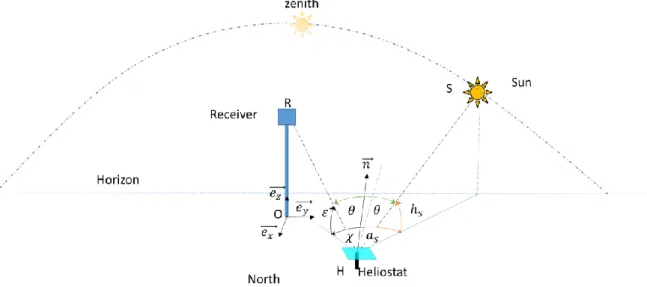
The analytical expression to compute the power P projected by a heliostat on the receiver can be found in [6]. It depends on the Direct Normal Irradiance (DNI) 𝐸𝑠𝑜𝑙 which varies with the day and weather,

the heliostat surface S and the orientation angle of the heliostat 𝜃 which can be derived from the different angles 𝑎_𝑠, ℎ_𝑠, 𝜀 𝑎𝑛𝑑 𝜒 defined in Figure 4.

𝑃 = 𝜂 𝐸_𝑠𝑜𝑙𝑆 cos𝜃 

The coefficient 𝜂 takes into account the heliostat efficiency and the atmospheric attenuation. Formula are proposed in the literature to compute the atmospheric attenuation, which depends on the distance between the heliostat and the receiver.

Figure 4 : Definition of sun angular position and incidence

The previous model is rather simple but it cannot be utilized in practice for several reasons.

The first reason is that there might be shading effects due to the tower or other heliostats which impact the light received by the heliostat. There might also be blocking effects when the direct line between the heliostat and the receiver meets another heliostat. These blocking and shading effects impact the power

P.

The second important reason is that this model only gives the total power received on the tower (in kW), but gives no information on the spatial distribution of the flux on the receiver (in kW/m²). Indeed, the light spot on the receiver is not a perfectly focused point. Reasons for this imperfect focusing are mainly because the sun cannot be assimilated to a point and because of the imperfections of the heliostats. The rays coming from the sun hit the heliostat in different points and are reflected in different directions such that the normal to the heliostat surface is the bisector of the angle between the incident and reflected ray.

The projection of the heliostat on the receiver is thus a fuzzy spot with rather ellipsoidal shape centered on the aiming point.

There are analytical models which take into account all aforementioned effects, such as HFLCAL or UNIZAR [8]. However, it is difficult to find the value for the many parameters of these models. The alternative approach we use is to model the heliostat field is using the data obtained with Tonatiuh and directly fit the flux map with Gaussian functions. Notice that this fitting approach can also be applied to real measurements of flux maps.

Gaussian distribution

The results of Tonatiuh simulations are the impact points of the rays on the receiver. For each heliostat, a statistic of this two-dimension data set can be computed.

We compute 𝜇 = (𝜇_𝑥, 𝜇_𝑦)𝑇 _{the mean value (barycenter of the energy) and Σ = [}𝜎𝑥 2 _𝜎

𝑥𝑦

𝜎𝑥𝑦 𝜎𝑦2

] the covariance matrix. With these parameters, the flux distribution is approximated by a Gaussian functions 𝜑 defined on the coordinate 𝑋 = (𝑥, 𝑦)𝑇 of the receiver plane:

𝜑(𝑥, 𝑦) = 1

2𝜋 √𝑑𝑒𝑡Σexp − 1

2(X − 𝜇)

𝑇_Σ−1_{(X − 𝜇)}

It can be mentioned that the covariance matrix Σ is an aggregation of the errors due to the sun diameter, the imperfection of the tracking and the imperfections of the mirror considered in the models found in the literature [8].

The function 𝜑 is a normalized distribution function which is multiplied by the power P to obtain the flux on the receiver plane:

Φ(x, y) = 𝑃. 𝜑(𝑥, 𝑦)

Parameterization

For a given heliostat, the power P and the covariance matrix Σ which characterizes the shape of the spot, depend only on the position of the sun given by the azimuth and elevation, not on the aiming points. Indeed, numerous fitting results showed us that: (i) center of the distribution 𝜇 is located at the aiming point and (ii) P and Σ are independent of the aiming point. Practically, this means that, when moving the aiming point, the flux distribution is translated but not distorted.

For the power P, the analytical expression given above can be the same as the value given by Tonatiuh if there are no shading or blocking effects, otherwise a correction must be made. The variance and covariance coefficients 𝜎_𝑥𝑦, 𝜎_𝑥, and 𝜎_𝑦 are computed for different positions of the sun and the results are interpolated with 2D polynomials of order 2×3.

Field model

The total flux Φtot on the receiver plane is obtained by adding the contributions of each heliostat where

and elevation angle of the sun, and (𝑥𝑎𝑝𝑖 , 𝑦𝑎𝑝𝑖 ) is the aiming point of each heliostat.

Φ_tot(x, y, 𝑎_𝑠, ℎ_𝑠, 𝑎𝑝) = ∑ 𝑃_𝑖(𝑎_𝑠, ℎ_𝑠). 𝜑_𝑖(𝑥 − 𝑥_𝑎𝑝𝑖 , 𝑦 − 𝑦_𝑎𝑝𝑖 , 𝑎_𝑠, ℎ_𝑠)

𝑁ℎ

𝑖=1

For keeping the notation compact, we name 𝑎𝑝 the set of all aiming points: 𝑎𝑝 = {𝑥_𝑎𝑝𝑖 _{, 𝑦}

𝑎𝑝𝑖 }𝑖=1..𝑁ℎ.

The integration of the 2D Gaussian being equal to one, 𝑃𝑟𝑒𝑓 the total power received by the infinite plane

containing the receiver surface is given by the equation: 𝑃_𝑟𝑒𝑓= ∑𝑁ℎ 𝑃_𝑖(𝑎_𝑠, ℎ_𝑠)

𝑖=1 .

However, the receiver is a limited five-by-five-meter square and a part of the flux reflected by the heliostat does not hit the receiver. The power received 𝑃_𝑡𝑜𝑡 is obtained by limiting the integration to the receiver surface:

𝑃_𝑡𝑜𝑡(𝑎𝑝) = ∬ Φ_tot(x, y, 𝑎_𝑠, ℎ_𝑠, 𝑎𝑝) 𝑑𝑥𝑑𝑦

𝑅𝑒𝑐𝑒𝑖𝑣𝑒𝑟 𝑆𝑢𝑟𝑓𝑎𝑐𝑒

Practically, this surface integral is computed numerically by dividing the receiver in 50x50 small squares. First results show a mean error between Tonatiuh and the approximation for the flux around 1%. Further analysis must be done to assess the precision of the model. However the model is much faster than the Tonatiuh model with a speedup factor 100. Finally, the proposed model is implemented in Matlab and can be integrated easily in optimization routines. This is also a major improvement over the original ray tracing model, since current version of Tonatiuh cannot be controlled by an external process (no API or command line automation).

AIMING POINTS OPTIMIZATION

Reference configuration

A natural strategy, if one wants to maximize the power, is to aim at the center of the receiver. The resulting flux is shown in Figure 5 for this reference configuration. The total power 𝑃_𝑡𝑜𝑡 is equal to 10.4 MW but the power is concentrated in a small part located around the center of the receiver. This aiming strategy leads to a high flux at the center (Φmax = 3793 kW/m²), which may not be compatible with

Figure 5 : Flux distribution in kW/m² for the reference configuration which maximizes the power 𝑷𝒕𝒐𝒕.

Multi objective Optimization

To avoid peak flux, the idea is to spread the received power without losing too much energy. This is a multi-objective optimization between loss and spread for which a mathematical formulation is proposed in the following.

Loss ratio. The loss ratio 𝐽_{𝐿𝑜𝑠𝑠} is defined below as the normalized lost power, a value between 0 and 1. Zero is the ideal value, but it cannot be reached due to imperfect focusing (as mentioned above, in the reference configuration for which they are minimum, losses are estimated to 4.7%).

𝐽𝐿𝑜𝑠𝑠 = 1 − 𝑃𝑡𝑜𝑡

𝑃𝑟𝑒𝑓 ,

𝑃𝑡𝑜𝑡, 𝑃𝑟𝑒𝑓 are defined in the previous paragraph.

Spread ratio. We first define the spread Δ Φ_𝑡𝑜𝑡 by the difference between the maximum and the minimum of the flux in kW/m2. This value is not dimensionless, so to facilitate the comparison with the loss criterion, it is normalized by its value in the reference configuration Δ Φ_𝑟𝑒𝑓. The spread ratio 𝐽_{𝑆𝑝𝑟𝑒𝑎𝑑} is again a number between 0 and 1. One is the worst value and it is attained in the reference configuration (all aiming point superimposed at the center).

𝐽𝑆𝑝𝑟𝑒𝑎𝑑 =

Δ Φ𝑡𝑜𝑡

Δ Φ𝑟𝑒𝑓

A spread of zero is the ideal value since it means that the flux would be uniformly distributed. However, we expect that for such a configuration the loss would be too big and inacceptable. So the aiming point strategy must find a compromise between the minimization of the loss and the spread ratio by the minimization of the combined criterion 𝐽_𝛼, where 𝛼 is a tuning factor.

x-coordinate (m) y-co o rd in a te ( m ) Flux Distribution kW/m2

Loss = 4.7107%, Dispersion = 1, Critere = 1 MaxFlux = 3793.2471, MinFlux = 1.3976 -2 -1 0 1 2 -2 -1.5 -1 -0.5 0 0.5 1 1.5 2 0 500 1000 1500 2000 2500 3000 3500

𝐽_𝛼 = 𝐽_{𝑆𝑝𝑟𝑒𝑎𝑑}+ 𝛼 𝐽_{𝐿𝑜𝑠𝑠}

Optimization Algorithms

The multi objective optimization defined in the previous section is a difficult problem without any analytical solution. A numerical optimization routine must be used to solve the problem. One can utilize unconstrained minimization algorithm or constrained optimization to take some constraints into account like forcing the aiming points to be inside the receiver. Specifically, we used fmin and fmincon from Matlab Optimization toolbox.

Two approaches are defined for the solving the optimization problem: a direct approach where optimization unknowns are the aiming points coordinates {𝑥_𝑎𝑝𝑖 _{, 𝑦}

𝑎𝑝𝑖 }𝑖=1..𝑁ℎ(2×108 real variables); an

indirect approach where optimization unknowns are the parameters of a parametric model (with a small number of parameters), the aiming points being computed with the parametric model. Notice that in this optimization section, we drop the “ap” indices from the aiming point variables for clarity.

Direct Approach.

The optimization problem is to find the aiming point heliostats coordinates 𝑥∗, y∗ in the receiver axes which minimize the objective function:

𝑥∗, y∗ = arg min

𝑥,𝑦 𝐽𝛼(𝑥, 𝑦)

Constraints can be added to limit the domain of research or to requirements for the solution.

The number of unknown is two times the number of heliostats (as there is one aiming point for each heliostat) which is a relatively important number, even for the small-sized field considered in the present paper.

To reduce the complexity of the optimization, we suppose that the problem can be decomposed in sub problems by considering smaller groups of heliostats. If we consider that the objective function is additive with respect to the heliostat contributions (this assumption implies that no coupling exists between the optimization variables resulting from blocking, shading, etc.) and that the objective function terms for each heliostat are positive, we can decompose the optimization.

min 𝑥,𝑦 𝐽𝛼(𝑥, 𝑦) = min𝑥𝑖,𝑦𝑖 ∑ 𝐽_𝛼(𝑥_𝑖, 𝑦_𝑖) 𝑁𝑔 𝑖=1 = ∑ min 𝑥𝑖,𝑦𝑖 𝑁𝑔 𝑖=1 𝐽_𝛼(𝑥_𝑖, 𝑦_𝑖)

Where (𝑥_𝑖, 𝑦_𝑖) are the aiming points for the heliostats of the ith group. We could consider that the way of creating the group is not important. It is true in theory but the function J is not convex and we might get stuck in a local minimum more easily with certain grouping configurations.

Indirect Approach

If we suppose that the minimum is unique, the optimization creates a mapping function from each heliostat given by its coordinate (X,Y) in the field coordinate shown in Figure 2 to the aiming points with coordinate (x,y) in the receiver coordinates. The idea of the indirect approach is to find a parametric model to make assumption on the mapping function by stating a parametric a priori model and optimize the parameters of the mapping function.

For instance, if (, ) are the polar coordinates of the heliostat, we can envisage the following mapping with two parameters A and B to be optimized and a fixed parameter k.

𝑥 = (Α𝜌 + 𝐵) cos(𝑘𝜃) 𝑦 = −(Α𝜌 + 𝐵) sin(𝑘𝜃) The optimization problem becomes:

𝐴∗, B∗ = arg min

𝐴,𝐵 𝐽𝛼(𝑥(𝐴, 𝐵), 𝑦(𝐴, 𝐵))

The dimension is dramatically reduced compared to the direct optimization.

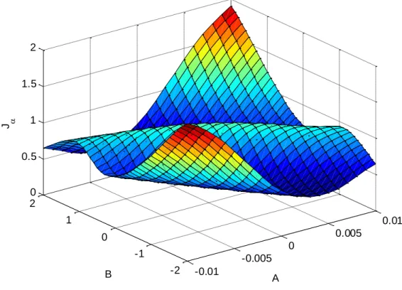
The objective function is more complex to compute and the convexity is no more guaranteed than in the direct approach as can be observed in Figure 6. The optimization is however two orders of magnitude faster than the direct approach. Of course, more complex mapping functions would lead to slower optimization, but better objective values.

Figure 6 : indirect method optimization function.

Results

The different optimization strategies described in the previous paragraphs were applied to the case study and are discussed in this paragraph.

The direct method optimized the entire field heliostats aiming points. The initial guess is chosen

-0.01 -0.005 0 0.005 0.01 -2 -1 0 1 2 0 0.5 1 1.5 2 A B J 

randomly. Several runs were made and the optimization generally ends with the maximum of iterations exceeded (n=100000), but results are acceptable even if the minimum is not reached.

The heliostat field is divided in four groups by taking shifted heliostat indices sets {1,5,9, …}, {2,6, ...}, {3,7,11, …}, {4,8,12, …}. Two initialization strategies have been adopted. The variant cold start assumes that the initial guess for each sub problem is chosen randomly. For the variant warm start the initial guess for the first group is chosen randomly and the solution of the optimization is chosen as a starting point for the next group, etc.

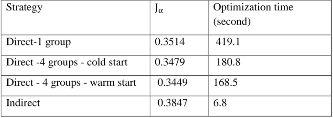
The results are given in Table 1. On the one hand, we can observe that the optimization time is divided by a speedup factor three by dividing the field in four groups and that the warm start does not bring significant improvement. On the other hand, a speedup factor 70 is obtained with the indirect approach. As the problem is non convex, several optimizations with randomly chosen starting point can be launched. With seven starting points, a speed up factor ten is obtained for the optimization - which can be performed in less than a minute. This appears to be sufficiently fast to be applied on line for control applications.

Strategy Jα Optimization time

(second)

Direct-1 group 0.3514 419.1

Direct -4 groups - cold start 0.3479 180.8 Direct - 4 groups - warm start 0.3449 168.5

Indirect 0.3847 6.8

Table 1 : optimization results

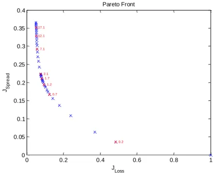
The Pareto front of the optimization with the indirect method is shown in Figure 7. We can see the effect of the parameter  on each objective. This parameter can be used as a tuning parameter to optimize the set points.

Figure 7 : Pareto front for the indirect optimization

5. CONCLUSION

A simple heliostat model is proposed for aiming point optimization. The flux distribution of each heliostat is approximated by a 2D-Gaussian model whose parameters are interpolated to obtain a model valid for all sun positions. To limit the complexity, the following assumptions are made. The center of the spot coincides with the aiming point. The vibration of the mirror caused by the wind (or other external disturbances) is neglected so that the aiming point set point is perfectly followed. A calibration procedure described in [6] must be done periodically to ensure this condition. The effect of blockage and shading between the heliostats are also neglected. The parameters of the 2D-Gaussian (x,xy,y) are identified

with data obtained with the Monte Carlo ray tracing software Tonatiuh. Identification procedures can also be applied with on-site measurement.

The optimization objective is to flatten as much as possible the flux distribution on the aperture plane and to simultaneously minimize the spillage. To quantify these objectives, two criteria for the spillage and the spread are defined. The heliostats aiming points are computed to minimize the multi objective function 𝐽_𝛼 . The parameter  can be adjusted to obtain the best compromise between the spillage and the spread.

In the perspective of designing a solution capable of modifying the aiming points in real time to take into account disturbances from the field - such as wind or clouds - or from the receiver - such as trip of pump or turbine - a fast solution was considered. Two approaches were adopted: the first one being to decompose the field in subsets of heliostats, the other one being to consider an a priori law for the aiming point and optimize the parameters of this mapping law. The mapping approach gives good results with an optimization done within a minute and is therefore a good candidate for on-line optimization.

0 0.2 0.4 0.6 0.8 1 0 0.05 0.1 0.15 0.2 0.25 0.3 0.35 0.4 0.2 0.7 1.2 1.7 2.1 7.1 12.1 17.1 Pareto Front J Loss J S p re a d

6. AKNOWLEGMENT

This work has been done in the frame of a collaboration with EDF China and IEE-CAS for the Badaling experimental platform. The authors would like to acknowledge the technical contributions of Supelec students Pan XuYang, Weicai Li, Paul Fino, and Baptiste Balique.

7. REFERENCE

[1] IEA, Technology Roadmap: Solar Thermal Electricity - 2014 edition

[2] D. Faille & al., Control Design Model for a Solar Tower Plant, Conf. SolarPaces 2013, Las Vegas, 2013

[3] D. Faille & al., Simulation Tools for Advanced Control Design and Hardware-In-The-Loop Verification, ISA, 2014

[4] S. Liu & al. Dynamic simulation of a 1MWe CSP tower plant with two-level thermal storage implemented with control system, Conf. SolarPaces 2014

[5] D. Faille & al., Control Solutions for Molten Salt Tower Concentrated Solar Plant, ISA, 2016 [6] E. Camacho & al., Advanced Control of Solar Plants, Springer Verlag

[7] A. Salomé, & al., Control of the flux distribution on a solar tower receiver using an optimized aiming point strategy: Application to THEMIS solar tower », Sol. Energy, vol. 94, p. 352 366, August 2013.

[8] A. Sánchez-González and D. Santana, « Solar flux distribution on central receivers: A projection method from analytic function », Renew. Energy, vol. 74, p. 576 587, February 2015.

[9] J. Zhang & al., Dynamic simulation of a 1MWe concentrated solar power tower plant system with Dymola®, Conf. SolarPaces 2013, Las Vegas, 2013