Predicting the Energy Consumption of MPI Applications at Scale Using a Single Node

HAL Id: hal-01523608

https://hal.inria.fr/hal-01523608v2

Submitted on 17 Jan 2019

HAL is a multi-disciplinary open access

archive for the deposit and dissemination of

sci-entific research documents, whether they are

pub-lished or not. The documents may come from

teaching and research institutions in France or

abroad, or from public or private research centers.

L’archive ouverte pluridisciplinaire HAL, est

destinée au dépôt et à la diffusion de documents

scientifiques de niveau recherche, publiés ou non,

émanant des établissements d’enseignement et de

recherche français ou étrangers, des laboratoires

publics ou privés.

Predicting the Energy Consumption of MPI

Applications at Scale Using a Single Node

Franz Heinrich, Tom Cornebize, Augustin Degomme, Arnaud Legrand,

Alexandra Carpen-Amarie, Sascha Hunold, Anne-Cécile Orgerie, Martin

Quinson

To cite this version:

Franz Heinrich, Tom Cornebize, Augustin Degomme, Arnaud Legrand, Alexandra Carpen-Amarie, et

al.. Predicting the Energy Consumption of MPI Applications at Scale Using a Single Node. Cluster

2017, IEEE, Sep 2017, Hawaii, United States. �hal-01523608v2�

Predicting the Energy Consumption of

MPI Applications at Scale Using a Single Node

Franz C. Heinrich, Tom Cornebize,

Augustin Degomme, Arnaud Legrand

firstname.lastname@imag.fr

Alexandra Carpen-Amarie

Sascha Hunold

Anne-Cécile Orgerie

Martin Quinson

CNRS/Inria/ENS Rennes, France firstname.lastname@irisa.fr

Abstract—Monitoring and assessing the energy efficiency of supercomputers and data centers is crucial in order to limit and reduce their energy consumption. Applications from the domain of High Performance Computing (HPC), such as MPI applications, account for a significant fraction of the overall energy consumed by HPC centers. Simulation is a popular approach for studying the behavior of these applications in a variety of scenarios, and it is therefore advantageous to be able to study their energy consumption in a cost-efficient, controllable, and also reproducible simulation environment. Alas, simulators supporting HPC applications commonly lack the capability of predicting the energy consumption, particularly when target platforms consist of multi-core nodes. In this work, we aim to accurately predict the energy consumption of MPI applications via simulation. Firstly, we introduce the models required for meaningful simulations: The computation model, the communication model, and the energy model of the target platform. Secondly, we demonstrate that by carefully calibrating these models on a single node, the predicted energy consumption of HPC applications at a larger scale is very close (within a few percents) to real experiments. We further show how to integrate such models into the SimGrid simulation toolkit. In order to obtain good execution time predictions on multi-core architectures, we also establish that it is vital to correctly account for memory effects in simulation. The proposed simulator is validated through an extensive set of experiments with well-known HPC benchmarks. Lastly, we show the simulator can be used to study applications at scale, which allows researchers to save both time and resources compared to real experiments.

I. INTRODUCTION

Supercomputers currently in use consume several megawatts of electrical energy per hour, making it an important goal to cut power consumption by finding the sweet spot between performance and energy consumption of applications run on these systems. Multi-core processors are responsible for a large fraction of the energy used by these machines and hence, exploiting power-saving techniques of these processors (e.g., Dynamic Frequency and Voltage Scaling (DVFS)) plays a crucial role.

When attempting to find trade-offs between performance and energy consumption on large-scale machines through experimentation, one faces a vast amount of configuration possibilities, e.g., number of nodes, number of cores per node, or DVFS levels. For that reason, a thorough experimental evaluation of the energy usage of HPC applications requires a large amount of resources and compute time. Simulation can help to answer the question of energy-efficiency, and

it has already been used to analyze HPC applications in a variety of scenarios. However, HPC simulators usually lack the capability to predict energy, although being able to study the effects of different DVFS policies may contribute to the understanding and the design of energy saving policies.

In this article, we address the problem of predicting the energy consumption of HPC applications through simulation. In particular, we show how to obtain energy predictions of MPI applications using the SimGrid toolkit. Energy usage in this context is modeled as the energy consumed by multi-core processors over the whole execution of the application, making an accurate prediction of the execution time of MPI appli-cations a basic requirement for a faithful prediction of their energy usage. Accurate predictions of performance and energy consumption of MPI applications could be highly beneficial for capacity planning, from both HPC platform designers and users’ perspectives, in order for them to adequately dimension their infrastructure.

The paper makes the following main contributions: 1) We first show how to predict (via emulation) the execu-tion time of MPI applicaexecu-tions running on a cluster of multi-core machines by using only a single node of that cluster for the emulation. More specifically, compared to our previous work in the context of SimGrid, our contribution addresses additional difficulties raised by the multi-core architecture of the nodes. In particular, we show that it is important to correctly model the two types of communications on such multi-core nodes, i.e., intranode (shared-memory) and intern-ode (MPI) communications as well as to account for the impact of memory/cache effects on computation time estimations in order to obtain reliable predictions of the energy consumption. 2) We propose and implement an energy model and explain how to instantiate it by using only a single node of a cluster. This model can later be used to predict the energy consumption of the entire cluster.

3) We demonstrate the validity of our model by showing that it can accurately predict both the performance and the energy of three MPI applications, namely NAS-LU, NAS-EP, and HPL.

4) We report pitfalls we encountered when modeling and calibrating the platform and that would lead to erroneous predictions when being overlooked.

providing evaluations of the amount of time (and energy) that can be saved by using simulations rather than real experiments to assess the performance of MPI applications.

The remainder of this article is organized as follows. Sec-tion II discusses related work, and SectionIIIintroduces our experimental setup. In SectionIV, we explain the models used within the SimGrid framework for predicting the computation and communication times, as well as the energy consumption of MPI applications. Section V presents how each of the involved models should be calibrated and instantiated to obtain faithful predictions. We evaluate the effectiveness of our approach in SectionVIbefore concluding in SectionVII.

II. RELATEDWORK

A. Energy Models for Compute Servers

In contemporary HPC nodes, processors are responsible for the lion’s share of the energy consumption [1]. The workload and the frequency of a CPU have a significant impact on its power usage [2]. The lower a processor’s frequency, the slower it computes but also the less energy it consumes.

Power models often break the power consumption of nodes into two separate parts: a static part representing the power consumption when the node is powered-on and idle; and a dynamic part that depends on the current utilization of the CPUs [3]. The static part can represent a significant percentage of the maximum power consumption. For that reason, turning off servers during idle periods can save significant amounts of energy [4]. The relationship between the power consumption and load (utilization) of a CPU is linear for a given application at a given frequency, as explained in [1].

For HPC servers experiencing only few idle periods, DVFS constitutes a favorable alternative to switching off machines. DVFS adapts the processor’s frequency according to the application workload and, for instance, can hence decrease the frequency during communication phases [5].

Power consumption of interconnects can account for up to 30 % of the overall power consumption of the cluster but it is generally fixed and independent of their activity, although some techniques for switching on and off links depending on traffic have been investigated [6]. The energy consumption of network cards (NICs) is often considered negligible for HPC servers, as it typically is responsible for only 2 % of the overall server’s consumption [3]. Furthermore, it usually does not exhibit large variations related to traffic [1]. Memory (e.g., DRAM), on the other hand, is accounts for a share of 20 % to 30 % of the power consumption of HPC nodes [3] and hence plays an important role.

Network cards and memory are typically accounted for in the static part of a server’s power consumption [1]. This static part also includes the power consumption of the nodes’ storage and other components.

B. Cloud and HPC Simulators

Energy optimization is a primary concern when operating a data center. Many simulators have been designed for a cloud context and include a power consumption model [7], [8]. For

example, Guérout et al. [9] extended CloudSim [10] with DVFS models to study cloud management strategies, while GreenCloud [11] is an extension of the NS2 simulator for energy-aware networking in cloud infrastructures. DCSim [8] is a simulation tool specifically designed to evaluate dynamic, virtualized resource management strategies, featuring power models that can be used to determine the energy used on a per-host basis.

However, as explained by Velho et al. [12], several simu-lation toolkits have not been validated or are known to suffer from severe flaws in their communication models, render-ing them ineffective in an HPC application-centric context. Simulators that use packet-level and cycle-level models are arguably realistic (provided that they are correctly instantiated and used [13]), but they suffer from severe scalability issues that make them unsuitable in our context.

Many simulators have been proposed for studying the performance of MPI applications on complex platforms, among others Dimemas [14], BigSim [15], LogGOPSim [16], SST [17], xSim [18] as well as more recent work such as CODES [19] and HAEC-SIM [20]. Most of these tools are designed to study or to extrapolate the performance of MPI applications at scale or when changing key network parameters (e.g., bandwidth, topology, noise). Surprisingly, only a few of them embed a sound model of multi-core architectures. A notable exception is Dimemas [14], which implements a network model that discriminates clearly between communi-cations within a node (going through shared memory) and communications that pass through the network. The PMAC framework [21] uses a rather elaborate model of the cache hierarchy and can be combined with Dimemas to provide predictions of complex applications at scale. However, both tools solely rely on application traces, which can be limiting in terms of scalability and scope.

To the best of our knowledge, none of these tools except HAEC-SIM embeds a power model or allows researchers to study energy-related policies. HAEC-SIM can process OTF2 application traces and can apply simulation models (communi-cation and power) that modify event properties. The simulation models are however quite specific to their envisioned use case and only cover a very small fraction of the MPI API. The validation is done at small scale (the NAS-LU benchmark with 32 processes), and although prediction trends seem very faithful and promising, 20 to 30 % of prediction errors in power estimation compared to reality are not uncommon.

III. EXPERIMENTALSETUP ANDMETHODOLOGY

In this work, we rely on the Grid’5000 [22] infrastructure, in particular on the Taurus cluster1_{, as each of its nodes is}

equipped with a hardware wattmeter. The measurements of these wattmeters are accessed through the Grid’5000 API, and power measurements are taken with a sampling rate of 1 Hz and an accuracy of 0.125 W.

1_{Technical specification at https://www.grid5000.fr/mediawiki/index.php/}

The Taurus cluster is composed of 16 homogeneous nodes, each consisting of 2Intel Xeon E5-2630CPUs with 6 phys-ical cores per CPU and 32 GiB of RAM. Each CPU has 3 cache levels of the following sizes: 32 KiB for L1, 256 KiB for L2 and 15 MiB for L3. These nodes are interconnected via 10 Gbit/ sec Ethernet links to the same switch as two other smaller clusters and a service network. In order to rule out any performance issues caused by other users, in particular regarding network usage, we reserved the two smaller clusters during our experiments as well. They are, however, not part of this study. We deployed our own custom Debian GNU/Linux images before any experiment to ensure that we are in full control of the software stack used. We used Open MPI 1.6.5 for our experiments, but our approach is independent of the specific MPI version used. Finally, unless specified otherwise, CPU frequency was set to 2.3 GHz.

We use three MPI applications in our study that are all CPU-bound for large enough problem instances. The first two originate from the MPI NAS Parallel Benchmark Suite (v3.3). The NAS-EP benchmark performs independent computations and calls threeMPI_Allreduceoperations at the end to check the correctness of the results. The NAS-LU benchmark solves a square system of linear equations using the Gauss-Seidel method and moderately relies on the MPI_Allreduce and

MPI_Bcast operations. Most of its communication patterns

are implemented through blocking and non-blocking point-to-point communications. Finally, we chose the HPL benchmark (v2.2), as it is used to rank supercomputers in the TOP500 [23] and in the Green500 lists.

To allow researchers to inspect and easily build on our work, all the traces and scripts used to generate the figures presented in the present document are available online2 as well as an extended version detailing the importance of experimental control3. Likewise, all the developments we have done have been integrated to the trunk of the open-source SimGrid simulation toolkit4_.

IV. PREDICTING THEPERFORMANCE OFMPI

APPLICATIONS: THESIMGRIDAPPROACH

Now, we present the main principles behind the simulation of MPI applications and explain more specifically in Sec-tionsIV-Aand IV-Bhow they are implemented in SimGrid, an open-source simulation toolkit initially designed for distributed systems simulation [24], which has been extended with the SMPI module to study the performance of MPI applica-tions [25]. Most efforts of the SimGrid development team over the last years have been devoted to comparing simulation pre-dictions with real experiments as to validate the approach and to improve the quality of network and application models. The correctness of power consumption prediction is particularly dependent on the faithfulness of runtime estimation, and so only recently, after the SMPI framework had successfully been validated with many different use cases [25], has it become

2 _{https://gitlab.inria.fr/fheinric/paper-simgrid-energy} 3 _{https://hal.inria.fr/hal-01446134}

4 _{http://simgrid.gforge.inria.fr/}

possible to invest in power models and an API to control them. This contribution will be detailed in SectionIV-C.

A. Modeling Computation Times

Two main approaches exist to capture and simulate the behavior of MPI applications: offline simulation and online simulation. In offline simulation, a trace of the application is first obtained at the level of MPI communication events and then replayed on top of the simulator. Such a trace comprises information about every MPI call (source, desti-nation, payload, . . . ) and the (observed) duration of every computation between two MPI calls. This duration is simply injected into the simulator as a virtual delay. If the trace contains information about the code region this computation corresponds to, correction factors can be applied per code region. Such corrections are commonly used in Dimemas [14] to evaluate how much the improvement of a particular code region would influence the total duration of the application.

In the online simulation approach the application code is executed and part of the instruction stream is intercepted and passed on to a simulator. In SimGrid, every MPI process of the application is mapped onto a lightweight simulation thread and every simulation thread is run in mutual exclusion from the others. Every time such a thread enters an MPI call, it yields to the simulation kernel and the time it spent computing (in isolation from every other thread) since the previous MPI call can thus be injected into the simulator as a virtual delay. This captures the behavior of the application dynamically but otherwise relies on the same simulation mechanisms used for replaying a trace. This form of emulation is technically much more challenging but is required when studying applications whose control flow depends on the platform characteristics, a property that is becoming more and more common. Note that this is actually the case for the HPL benchmark: It relies heavily on the MPI_Iprobe operation to poll for panel reception during its broadcast while overlapping the time for the transfer with useful computations. The main drawback of this approach is that it is usually quite expensive in terms of both simulation time and memory requirements since the whole parallel application is actually executed on a single host machine. SMPI provides simple computation (sampling) and memory (folding) annotation mechanisms that make it possible to exploit the regularity of HPC applications and to drastically reduce both memory footprint and simulation duration [25]. The effectiveness of this technique will be illustrated in SectionVI-B.

The online and the offline approach are implemented within SimGrid’s SMPI layer. The SMPI runtime layer mimics the be-havior of MPI in terms of semantic (synchronization, collective operations) and supports both emulation (online simulation) and trace replay (offline simulation). This organization allows users to benefit from the best of both worlds (e.g., using a lightweight replay mechanism combined with a dynamic load balancing [26] or easily implementing complex collective communication algorithms [25]). The price to pay compared to a simulator solely supporting offline simulation (e.g.,

Log-Figure 1. Communication time between two nodes of the Taurus cluster (Ethernet network). The duration of the communication with eitherMPI_Send

orMPI_Recvare modeled as piece-wise linear functions of the message size.

GOPSim [16]) is that the SMPI replay mechanism systemati-cally relies on simulation threads but careful optimizations can drastically limit this overhead [27], [25].

A few other tools, e.g., SST [17] and xSim [18], support online simulation and mostly differ in technical implementa-tion (emulaimplementa-tion mechanism, communicaimplementa-tion models, etc.) and coverage of the MPI standard. SMPI implements the MPI-2 standard (and a subset of the 3 standard but for MPI-IO) and allows users to execute unmodified MPI applications directly on top of SimGrid.

B. Modeling Communication Times

Several challenges arise when modeling communication of MPI applications. The first one is caused by the complex network optimizations done in real MPI implementations. Dif-ferent transmission protocols (short, eager, rendez-vous) may be used depending on the message size. This incurs different synchronization semantics even when using blocking Send and Receive operations (e.g., for short messages, MPI_Send

generally returns before the message has actually been deliv-ered to the receiver). Additionally, the low-delay high-latency network layer (e.g., Infiniband, Omnipath, TCP/IP, . . . ) relies on different mechanisms, which leads to very different effec-tive latency and bandwidth values depending on message size. To capture all such effects, SMPI relies on a generalization of the LogGPS model [25] where several synchronization and performance modes can be specified (see Figure 1). The calibration procedure of such a model consists of sending a series of messages viaMPI_SendandMPI_Recv, with carefully randomized sizes, between two nodes and to fit piece-wise linear models to the results with theRstatistical language5_{. As}

illustrated in Figure1, at least five modes can be distinguished depending on message size and correspond not only to differ-ent synchronization modes but also to varying performances. The protocol switches from one mode to another could clearly be optimized, but this behavior is not unusual and more than five modes are commonly found for TCP Ethernet networks.

The second key challenge is related to the modeling of net-work topology and contention. SMPI builds on the flow-level models of SimGrid and models communications, represented

5_{Seehttps://gitlab.inria.fr/simgrid/platform-calibrationfor more details.}

Averageidleconsumption(Pidle) Pstatic 0 50 100 150 200 250 0 1 4 8 12

Number of active cores

P o w er (W atts) Frequency (MHz) 1200 1400 1600 1800 2000 2200

Taurus cluster, Lyon, NAS−EP

Figure 2. Power consumption ontaurus-8when running NAS-EP, class C, varying the frequency and the number of active cores.

by flows, as single entities rather than as sets of individual packets. Assuming steady-state, the contention between active communications is modeled as a bandwidth sharing problem that accounts for non-trivial phenomena (e.g., RTT-unfairness of TCP, cross-traffic interference or simply network hetero-geneity [12]). Every time a communication starts or ends, the bandwidth sharing has to be recomputed, which can be too slow and complex to scale to large platforms. However, this approach not only leads to significant improvements in simulation accuracy over classical delay models but can also be efficiently implemented [28].

Finally, the third challenge is incurred by MPI collec-tive operations which are generally of utmost importance to application performance. Performance optimization of MPI collective operations has received significant attention. MPI implementations thus have commonly several alternatives for each collective operation and select one at runtime depending on message size and communicator geometry. For instance, in Open MPI, theMPI_Allreduceoperation spans about 2300 lines of code. Ensuring that any simulated run of an applica-tion uses the same (or a comparable) implementaapplica-tion as the real MPI implementation is thus key to simulation accuracy. SimGrid’s SMPI layer implements all the specific collective communication algorithms from several real MPI implementa-tions (e.g., Open MPI, MPICH, . . . ) and their selection logic. SMPI can hence account for performance variation based on the algorithm used for collective communications, allowing researchers to investigate a multitude of environments and configurations. Note that the applications we study in the following mostly rely on their own pipelined implementation of collective operations.

C. Modeling the Energy Consumption of Compute Nodes Power consumption of compute nodes is often modeled as the sum of two separate parts [1]: a static part that represents the consumption when the server is powered on but idle; and a dynamic part, which is linear in the server utilization and depends on the CPU frequency and the nature of the com-putational workload (e.g., computation vs. memory intensive, provided such characterization can be done). Therefore, we use the following equation to model the power consumption for a

taurus−13 taurus−14 taurus−16

taurus−7 taurus−8 taurus−10 taurus−11 taurus−12 taurus−1 taurus−3 taurus−4 taurus−5 taurus−6

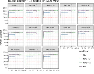
0 25 50 75 100 0 25 50 75 100 0 25 50 75 100 0 25 50 75 100 0 25 50 75 100 0 50 100 150 200 250 0 50 100 150 200 250 0 50 100 150 200 250 Time (s) P o w er (W atts) Workload Idle NAS−EP NAS−LU HPL

Taurus cluster − 13 nodes @ 2300 MHz

Figure 3. Power consumption over time when running NAS-EP, NAS-LU, HPL or idling (with 12 active cores and the frequency set to 2300 MHz).

given machine i, a frequency f , a computational workload w (HPC application), and a given usage u (in percentage):

Pi,f,w(u) = Pi,fstatic+ P dynamic

i,f,w × u . (1)

The linearity of our model is confirmed by measurements (see Figure 2). The parameters of the model in Equation (1) (Pstatic

i,f and P dynamic

i,f,w ) can be inferred from running the target workload twice: At first using only one core and consequently all cores of the CPU. The values in between are then interpo-lated. Note that the measurements of Figure 2show that it is generally safe to assume Pstatic

i,f is independent of the frequency but that it should not be confused with the fully idle power consumption Pidle_{. This can be explained by the fact that when} a CPU goes fully idle, it can enter a deeper sleep mode, which reduces its power consumption further.

When simulating an MPI application (either online or offline), it is easy to track whether a core is active or not, which allows the simulator to compute the instantaneous CPU usage (e.g., if 6 out of 12 cores of a given node are active, one would consider the load u to be 50 %) and to compute the integral of the resulting instantaneous power consumption to yield the total energy consumed by the platform. Such a model implicitly assumes that all cores either run a similar workload w or are idling, which is generally true as HPC applications are regular. Figure3illustrates this regularity and how the workload (independent executions of the NAS-EP or of NAS-LU with all cores used of each node) influences power consumption at a macroscopic scale.

Subsequently, we therefore assume that this computational workload is constant throughout the execution of the appli-cation and is known at the beginning of the simulation. If the application consists of several phases of very different nature, they should be independently characterized. Note that such characterization can be quite difficult to make if switches from one mode to another occur quickly since making

micro-estimations of such operations requires extremely fine tracing and power measurement tools that are rarely available.

V. MODELING ANDCALIBRATINGPERFORMANCE AND

ENERGYCONSUMPTION OFMULTI-CORECLUSTERS

We now present how the SMPI framework was extended to provide faithful makespan and power consumption predictions and how important the calibration of the platform is.

A. Computations: Unbiasing Emulation for Multi-core CPUs 1) Problem: All previously published work on the valida-tion of SMPI focused on networking aspects and hence used solely one core of each node. In this section, we explain two flaws of the SMPI approach that were particularly problematic when handling multi-core architectures and that we had to overcome in order to obtain accurate predictions.

(a) In SimGrid, computing resources are modeled by a capacity (in FLOP/s) and are fairly shared between the pro-cesses at any point in time.6 _{Hence, when p processes run}

on a CPU comprising n cores of capacity C, if p ≤ n, each process progresses at rate C while if p > n, each process progresses at rate Cn/p. Although such a model is a reasonable approximation for identical CPU bound processes, it can be wildly inadequate for more complex processes. In particular, when several processes run on different cores of the same node, they often contend on the cache hierarchy or on the memory bus even without explicitly communicating. It is thus essential to account for the potential slowdown that the computations of the MPI ranks may inflict on each others.

(b) As we explained in Section IV-A, SMPI’s emulation mechanism relies on a sequential discrete-event simulation kernel that controls when each process should be executed and ensures they all run in mutual exclusion between two MPI calls. When MPI applications are emulated with SMPI, each MPI rank is mapped onto a thread and folded within a single UNIX process, which raises semantic issues and requires to privatize global variables. This is done by making a copy of the data memory segment for each rank and by leveraging the virtual memory mechanism of the operating system to

mmap this data segment every time we context-switch from one rank to another. Since ranks run in mutual exclusion, the time elapsed between two MPI calls can be measured and dynamically injected into the simulator. If the architecture the simulation is run on is similar to the target architecture, we generally expect that this timing is a good approximation of what would be obtained when running in a real environment. Unfortunately, the combination of dynamic computation time measurement and of a simplistic computation model can lead to particularly inaccurate estimations. Let us consider on the one hand a target application consisting of many small computation blocks heavily exploiting the L1 cache and interspersed with frequent calls to MPI (for example to ensure communication progress). Each MPI call would result 6_{Note that the same property also holds for network links, which are fairly}

28 ...

Region 43if( iex .eq. 0 )then

30 Region 43 if( north .ne. -1 )then callMPI_RECV( dum1(1,jst),

32 > 5*(jend-jst+1), > dp_type, 34 > north, > from_n, 36 > MPI_COMM_WORLD, > status, 38 > IERROR ) Region 2 doj=jst,jend 40 Region 2 g(1,0,j,k) = dum1(1,j) Region 2 g(2,0,j,k) = dum1(2,j) 42 Region 2 g(3,0,j,k) = dum1(3,j) Region 2 g(4,0,j,k) = dum1(4,j) 44 Region 2 g(5,0,j,k) = dum1(5,j) Region 2 enddo 46 Region 2 endif Region 2

48 Region 2 if( west .ne. -1 ) then callMPI_RECV( dum1(1,ist),

50 > 5*(iend-ist+1), > dp_type, 52 > west, > from_w, 54 > MPI_COMM_WORLD, > status, 56 > IERROR ) Region 3 doi=ist,iend

58 Region 3 g(1,i,0,k) = dum1(1,i)

Region 3 g(2,i,0,k) = dum1(2,i)

60 Region 3 g(3,i,0,k) = dum1(3,i)

Region 3 g(4,i,0,k) = dum1(4,i)

62 Region 3 g(5,i,0,k) = dum1(5,i)

Region 3 enddo

64 Region 3 endif

...

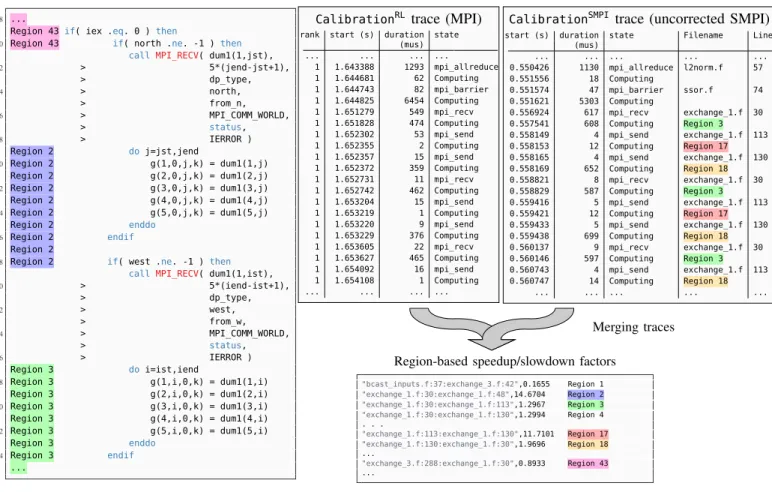
Figure 4. Excerpt of the NAS LU-PB (exchange_1.f) highlighting code regions between any two MPI cals.

CalibrationRL trace (MPI)

rank start (s) duration state (mus) ... ... ... ... 1 1.643388 1293 mpi_allreduce 1 1.644681 62 Computing 1 1.644743 82 mpi_barrier 1 1.644825 6454 Computing 1 1.651279 549 mpi_recv 1 1.651828 474 Computing 1 1.652302 53 mpi_send 1 1.652355 2 Computing 1 1.652357 15 mpi_send 1 1.652372 359 Computing 1 1.652731 11 mpi_recv 1 1.652742 462 Computing 1 1.653204 15 mpi_send 1 1.653219 1 Computing 1 1.653220 9 mpi_send 1 1.653229 376 Computing 1 1.653605 22 mpi_recv 1 1.653627 465 Computing 1 1.654092 16 mpi_send 1 1.654108 1 Computing ... ... ... ...

CalibrationSMPI trace (uncorrected SMPI)

start (s) duration state Filename Line (mus) ... ... ... ... ... 0.550426 1130 mpi_allreduce l2norm.f 57 0.551556 18 Computing 0.551574 47 mpi_barrier ssor.f 74 0.551621 5303 Computing 0.556924 617 mpi_recv exchange_1.f 30 0.557541 608 Computing Region 3 0.558149 4 mpi_send exchange_1.f 113 0.558153 12 Computing Region 17 0.558165 4 mpi_send exchange_1.f 130 0.558169 652 Computing Region 18 0.558821 8 mpi_recv exchange_1.f 30 0.558829 587 Computing Region 3 0.559416 5 mpi_send exchange_1.f 113 0.559421 12 Computing Region 17 0.559433 5 mpi_send exchange_1.f 130 0.559438 699 Computing Region 18 0.560137 9 mpi_recv exchange_1.f 30 0.560146 597 Computing Region 3 0.560743 4 mpi_send exchange_1.f 113 0.560747 14 Computing Region 18 ... ... ... ... ... Merging traces Region-based speedup/slowdown factors

"bcast_inputs.f:37:exchange_3.f:42",0.1655 Region 1 "exchange_1.f:30:exchange_1.f:48",14.6704 Region 2 "exchange_1.f:30:exchange_1.f:113",1.2967 Region 3 "exchange_1.f:30:exchange_1.f:130",1.2994 Region 4 . . . "exchange_1.f:113:exchange_1.f:130",11.7101 Region 17 "exchange_1.f:130:exchange_1.f:30",1.9696 Region 18 ... "exchange_3.f:288:exchange_1.f:30",0.8933 Region 43 ...

Figure 5. Trace merging process used for the NAS-LU benchmark to compute region-based speedup/slowdown factors and correct the simulation.

in injecting the duration of the preceding computation into the simulator and immediately yielding to another rank. Despite all the care we took in implementing efficient and lightweight context switches, the content of the L1 cache will be cold for the new rank and its performance will therefore be much lower than it would have had if it was running on its dedicated core (i.e., with dedicated L1 cache). Our emulation may therefore be biased, resulting in a significant apparent slowdown for such applications.

On the other hand, let us consider a target application consisting of relatively coarse-grained computation blocks which shall be considered to be memory-bound, i.e., that contend on L3 or on the memory bus when using all the cores of the machine. Since we measure each computation in mutual exclusion, during the simulation each rank benefits from an exclusive access to the L3 cache and the computation times injected in the simulation will thus be very optimistic com-pared to what they would have been in a real-life execution.

Obviously, real HPC codes comprise both kinds of situations and knowing beforehand whether a given code region will be sped up or slowed down during the emulation compared to the real execution is very difficult as it is dependent on both the memory access pattern and the memory hierarchy.

2) Solution: To unbias our emulation and characterize the true performance of the application, we first run the application

with a small workload using all the cores of a single node. This real-life (RL) execution is traced as lightly as possible at the MPI level and the duration of every computation is recorded (CalibrationRL in Figure 5). We then re-execute the application with the exact same workload but on top of the SimGrid (SMPI) simulator (hence using a single core, possibly even on another machine) and trace accordingly the duration of every computation as well as the portion of code it corresponds to (CalibrationSMPI in Figure 5). We propose to identify the origin of the code by the filename and the line numbers of the surrounding two MPI calls as it can be obtained during compilation and therefore incurs a minimal overhead during the simulation (see Figure 4). Such identification of code regions may be erroneous, for example when MPI calls are wrapped in the application through some portability layer (in fact, this is the case for HPL). In this case, it might be required to identify code regions by the whole call-stack, as done for instance by SST/DUMPI [17]. Yet, as we will see, such level of complexity was not needed in our cases.

Since the application code is emulated by SimGrid, the duration of computations in CalibrationRL may be quite different from the ones in CalibrationSMPI, as we dis-cussed above. We automatically align theCalibrationRL and

CalibrationSMPI traces (see Figure 5) with an R script and

NAS−LU ● Reality Simulation (corrected) Simulation (uncorrected) Ideal scaling ● ● ● ● 0 50 100 1x12 4x12 8x12 12x12 Run−time (in s) ● ● ● ● 0 10 20 30 40 50 1x12 4x12 8x12 12x12 Energy (in kJ)

nodes x processes per node

Figure 6. Illustrating the importance of unbiasing the emulation when simulating multi-core CPUs, NAS-LU, class C.

that should be applied when emulating the target application. For a given code region c, this factor is defined as the ratio of the total time over all ranks spent in c inCalibrationSMPI to the total time over all ranks spent in c inCalibrationRL. This factor then enables SimGrid to scale dynamically measured computation times accordingly.

Figure 5 depicts an excerpt of a file resulting from the calibration of computations. This file serves as input to SMPI and is used to correctly account for the duration of the computations on the target architecture. Some code regions have a speedup factor of around 1.29, which means that the duration of the corresponding code is actually faster when emulating than when running in a normal environment, while some other code regions have a speedup around 0.9, which means they are slower when being emulated.

3) Effectiveness of the Solution: For some applications, like computation-bound NAS-EP or for HPL, we found that most factors are very close to 1 and this correction has therefore al-most no impact on the overall makespan prediction. However, for a memory-bound code like NAS-LU, not accounting for slowdowns and speedups of code regions leads to an overall runtime estimation error of the magnitude of 20 to 30 % (see Figure 6) and hence to a major energy-to-solution estimation error.

It is interesting to note that some code regions (e.g., the first one in Figure 5) can have very low speedup factors while others (e.g., the second one) can have large and hence important speedup factors. In our experience, the ones with low speedup factors are seldom called (e.g., only once per rank) while the ones with large speedup factors have very frequent calls (possibly hundreds of thousands) but a very short duration. In both cases, their impact on the overall simulated time is negligible.

4) Limitations: Aside from the region identification that could be implemented more robustly, this method implicitly assumes that the correction factors determined for a single node still hold when the application spans several nodes. Intu-itively, these correction factors are governed by cache locality and reuse and may thus be quite sensitive to problem size. The approach should therefore naturally work when conducting weak scaling studies but could break when conducting strong scaling studies. Yet, as can be seen for the previous example

Figure 7. Communication time between two CPUs of the same node of Taurus (i.e., over shared memory). Compared to Figure1, communications are not only less noisy but can also be almost one order of magnitude faster for large messages. Small messages appear faster over network links than over shared memory because they are sent asynchronously (the duration ofMPI_Sendand

MPI_Senddoes not account for transmission delay).

HPL ● _{Reality Simulation (calibrated) Simulation (loopback same as ethernet)}

Ideal scaling ● ● ● ● 0 25 50 75 1x12 4x12 8x12 12x12 Run−time (in s)

nodes x processes per node

Figure 8. Comparison of simulation results for HPL between a correctly calibrated simulation and simulation that would not account for specific shared memory communication characteristics.

(Figure 6), where the class of the problem is fixed, this did not happen in our experiments so far. This may be explained by the fact that the code is relatively well optimized and that there is thus no significant difference between the correction factors obtained when using class C or a smaller workload. B. Communications: Local Communications

1) Problem: As explained in SectionIV-B, the communica-tion model implemented in SMPI is a hybrid model between the LogP family and a fluid model that takes into account whether messages are sent fully asynchronously, in eager mode or synchronously. Switches from one mode to another depend on message size and the resulting performance can be modeled through a piece-wise linear model with as many pieces as needed (5 modes in Figure 1). Unfortunately, the model presented in Section IV-B only makes sense for (remote) communications between distinct nodes. Communications that remain internal to a node use shared memory rather than the network card and it is therefore common to observe not only largely different performances, but also slightly different be-haviors (protocol changes are determined by different message sizes and the regressions are expected to be different).

2) Solution: A series of measurements similar to the mea-surements used for the network was run on two cores of the

same node to calibrate the model for local communications (see Figure 7) accordingly. Although they are much more stable, simpler and more efficient than remote communi-cations, using a completely different model to distinguish between local and remote communications turned out to be of little importance because the applications we considered for this work do not exploit locality and communication is dominated by remote communications. Communications over memory were therefore simply modeled by a 40 Gbit/ sec shared link, which supports accounting for both contention and heterogeneity. Applications without these properties need to be investigated in the future as they were beyond the scope of this work.

3) Effectiveness of the solution: We illustrate the conse-quences of distinguishing between local and remote commu-nications with the HPL benchmark. As can be seen in Fig-ure 8, ignoring heterogeneity (blue dotted line) is particularly misleading at small scale since it incurs an overall runtime estimation error of the magnitude of 25 % whereas accounting for fast local links (green dashed line) provides a perfect prediction at any scale. Since this modeling error solely incurs additional communication and idle times, the additional power consumption remains relatively small compared to the full load consumption of pure computations. The prediction error is thus around a few percents (even when there is a 25 % error in runtime) and is within the variability of real experiments. The version of HPL we used does not specifically exploit locality, and hence, as soon as more than one node is used, the whole application gets slowed down by the less performant Ethernet links and the runtime and power estimations become equivalent to the ones obtained when correctly modeling network heterogeneity.

4) Limitation: When comparing Figures1and7it appears that, although the common modes can be found, the regres-sions differ largely. Ideally, to faithfully predict the behavior of applications that are highly sensitive to communications and potentially use the whole spectrum of message sizes, we should allow SimGrid users to model completely different latency/bandwidth correction factors that would then be se-lected depending on what group of nodes is communicating. Support for this is underway and will leverage the hierarchical platform representation of SimGrid [27]. Nevertheless, in all the experiments we conducted so far, correct evaluation of the effective latency and bandwidth of shared memory communications was all that was needed in order to obtain faithful predictions.

It should be noted that if the network topology is known or expected to be decisive (as it was the case in [25], where a much more contended network topology was considered), then some network saturation experiments should be done to properly evaluate where bottlenecks may occur. We ran such experiments for consistency but as our cluster is of limited size with a well provisioned router, a flat topology was sufficient. Finally, one should make sure that the same collective communication selector is used for both real-life experiments and the simulation. In our case, the impact of this particular

taurus−11 taurus−12 taurus−16

taurus−3 taurus−4 taurus−5 taurus−7

0 200 400 600 0 200 400 600 0 200 400 600 0 200 400 600 90 100 110 120 90 100 110 120 Time (s) P o w er (W atts) Date 2014−05−05 2016−11−23

Taurus cluster, Idle consumption − 7 nodes @ 2300 MHz

Figure 9. Idle power consumption along time when the frequency is set to 2300 MHz for several nodes of the Taurus cluster in 2014 and in 2016. The Y-axis does not start at 0 to provide a better appreciation of the variations.

configuration is limited as well, as the applications that we used to evaluate our new models barely rely on collective communications.

C. Energy: Heterogeneity and Communication Polling 1) Problem: Although it is typically assumed that a cluster is homogeneous, a systematic calibration of the whole cluster often demonstrates this to be false [29]. For illustration, Figure 9 depicts the power consumption along time on two different dates (May 2014 and October 2016) for various nodes. Not only can one observe significant differences be-tween nodes, but the power consumption oftaurus-12has for instance increased by 11 W whereastaurus-5now consumes 3 W less. In 2014, the cluster could have been considered as homogeneous but in 2016, this has evidently not been the case anymore. These measurements are, however, quite stable. Over the experiment duration of two hours, a few outliers (around 0 W or 50 W) per node were easily detected and removed as they could be attributed to powermeter glitches. The sample mean is thus a very good approximation of the distribution and we calibrated our models accordingly. Although not everyone may want or is even able to conduct a large scale calibration of the platform, monitoring infrastructures are generally deployed on large platforms and can be used to detect nodes that behave differently and require individual calibration. This kind of heterogeneity remains limited (within a few percents of the overall capacity since Pstatic_{is typically around 92 W) and can} easily be provided to SimGrid if needed. Yet, in our experi-ments, accounting for the heterogeneity of the platform only incurred ≈ 1 % of difference, which makes it indistinguishable from the noise of real experiments.

More importantly, as noted in SectionIV-C, although Pstatic i,f does not appear to depend on the frequency, it should neither be confused with the fully idle power consumption Pidle nor with the "turned-off" power consumption or with the power consumption during the boot procedure. These different states lead to very different behaviors and should all be characterized if a power estimation of the whole cluster under a mixed work-load is expected. Every such state and every new application

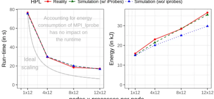
HPL ● Reality Simulation (w/ iProbes) Simulation (wo/ iprobes) Ideal scaling ● ● ● ● 0 20 40 60 80 1x12 4x12 8x12 12x12 Run−time (in s) ● ● ● ● 0 10 20 30 1x12 4x12 8x12 12x12 Energy (in kJ)

nodes x processes per node Accounting for energy

consumption of MPI_Iprobe has no impact on

the runtime

Figure 10. Comparison of predicted energy usage of HPL with and without accounting for the additional energy consumption of MPI_Iprobe calls.

requires a specific series of potentially tedious measurements. However, in our opinion, they can hardly be avoided. Alas, some of these "states" can at times be rather difficult to anticipate. For example, the MPI_Iprobeoperation is actually not used by the NAS benchmarks but heavily used by HPL in its custom re-implementation of broadcast operations that support efficient overlapping with computations. In our earlier versions of SMPI we had already taken care of measuring the time it takes to execute a call to MPI_Iprobe. However, the resulting call was simply modeled as a pure delay, hence leaving the simulated core fully idle for a small period of time. However, when HPL enters a particular region with intense communication polling, constantly looping over MPI_Iprobe

actually incurs some non-negligible CPU load that can lead to significant power estimation inaccuracies if not modeled correctly.

2) Solution: We have extended our benchmark of

MPI_Iprobe and it now detects what energy consumption is

incurred by repeated polling. For example, when all the cores of a node are polling communications, the power consumption was measured to be around 188 W, which is lower than the power consumption incurred by running for example HPL (≈214 W at maximal frequency) on the whole node but much higher than the idle power consumption (≈110 W). We have therefore extended SMPI so that this power consumption can be specified and be accounted for.

3) Effectiveness of the solution: Figure10depicts how the time-to-solution and energy-to-solution of HPL evolve when adding more resources. Since the network performance and the average duration of the MPI_Iprobe have been correctly instantiated, the run-time prediction matches perfectly the ones of real executions. When modeling the MPI_Iprobe as a pure delay, the resulting core idleness leads to a gross underestimation of energy consumption (blue dotted line). Fortunately, correctly accounting for the power consumption of the MPI_Iprobe operation ensures that perfect predictions (green dashed line) of the total energy consumption are yielded.

VI. EVALUATION

A. Validation Study

In the previous section, we explained how important it can be to correctly account for various effects and to correctly

NAS−EP ● Reality Simulation

Ideal scaling ● ● ● ● 0 10 20 30 40 50 1x12 4x12 8x12 12x12 Run−time (in s) ● ● ● ● 0.0 2.5 5.0 7.5 1x12 4x12 8x12 12x12 Energy (in kJ)

nodes x processes per node

NAS−LU ● Reality Simulation

Ideal scaling ● ● ● ● 0 25 50 75 100 1x12 4x12 8x12 12x12 Run−time (in s) ● ● ● ● 0 10 20 30 1x12 4x12 8x12 12x12 Energy (in kJ)

nodes x processes per nodeHPL ● Reality Simulation

Ideal scaling ● ● ● ● 0 20 40 60 80 1x12 4x12 8x12 12x12 Run−time (in s) ● ● ● ● 0 10 20 30 1x12 4x12 8x12 12x12 Energy (in kJ)

nodes x processes per node

Figure 11. Validating simulation results for NAS-EP, NAS-LU, and HPL, on up to 12 nodes with 12 processes per node.

instantiate the different models. We recap in Figure 11 the comparison of careful simulations with real executions for the three applications presented earlier: NAS-EP, NAS-LU and HPL. In all cases, the performance prediction is almost indistinguishable from the outcome of the real experiments.

Although the previous general behavior is somehow ex-pected (perfect speedup for EP but sub-linear for NAS-LU and HPL which causes an increasing energy consumption), we manage to systematically predict both performance and power consumption within a few percents.

B. Scalability and Extrapolation

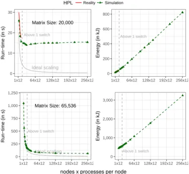
To illustrate the benefits of such a simulation framework, we performed a strong scaling of HPL on a hypothetical platform made of 256 12-core CPUs similar to the ones of the Taurus platform but interconnected with a two level fat-tree made of 16-port switches and where the top (resp. bottom) layer comprises 2 (resp. 16) switches and 10 Gbit/ sec Ethernet links.

Previous validation experiments leveraged solely the default emulation mechanism that allows users to evaluate unmod-ified MPI applications. In this mode, every computation of each process is performed. At scale, this quickly becomes

HPL Reality Simulation Matrix Size: 20,000 Ideal scaling Above 1 switch 0 10 20 30 1x12 64x12 128x12 192x12 256x12 Run−time (in s) ●●●● Above 1 switch 0 200 400 600 800 1x12 64x12 128x12 192x12 256x12 Energy (in kJ) Matrix Size: 65,536 Ideal scaling Above 1 switch 0 250 500 750 1,000 1,250 1x12 64x12 128x12 192x12 256x12 Run−time (in s) Above 1 switch 0 1,000 2,000 3,000 1x12 64x12 128x12 192x12 256x12 Energy (in kJ)

nodes x processes per node

Figure 12. Extrapolating time- and energy-to solution on a fat-tree topology with up to 256 × 12 = 3, 072 MPI processes.

prohibitive and generally requires much more time than a real-life execution since all MPI processes are then folded on a single machine. As an illustration, running HPL for real on 144 cores with a 20, 000 × 20, 000 matrix (i.e., with a memory consumption of 3.2 GB in total) requires less than 20 seconds whereas a full emulation requires almost two hours. However, as explained in Section IV-A, since HPC applications are very regular, it is possible to drastically reduce this cost by modeling the duration of computation kernels (hence skipping their execution during the emulation) and folding memory allocations (hence reducing the memory footprint). With such mechanisms in place, it is possible to simulate the same scenario (a 20, 000 × 20, 000 matrix with 144 processes) on a single core of a commodity laptop in less than two minutes using 43 MB of memory. Simulating an execution with 256 × 12 = 3, 072 MPI processes requires about one hour and a half and less than 1.5 GB of memory.

Figure 12 depicts a typical scalability evaluation when the matrix size is fixed to either 20,000 (3.2 GB in total) or 65,536 (34.3 GB). With the smaller matrix, this quickly leads to a fully network bound scenario where a slowdown is expected. The values obtained with up to 12 nodes (144 processes) are perfectly coherent with real-life experiments since the application is executed on nodes connected to the same switch. When spreading over more than one switch (i.e., above 196 processes), however, the additional latency becomes a hindrance, which leads to both a slowdown and an even faster increase of power consumption. For the larger matrix, we expected and observed a better scaling. Energy consumption is larger not only because the whole duration is larger but also because the ratio of communication to computations is very different.

VII. CONCLUSIONS

Predicting the energy usage of MPI applications through simulation is a complex problem. In the present article, we have taken first steps towards solving this problem. We have described the models that can be used to predict the compu-tation and communication time of MPI applications, as these models form the basis for our simulator to predict the energy consumption. Despite the simplicity of these models, obtaining accurate predictions is not a straight-forward task. Instead, each model needs to be carefully instantiated and calibrated. To that end, we have identified several key elements that need to be accounted for in this calibration process. The advantage of our simulation process is that we can obtain accurate predictions by using only one node of a (homogeneous) compute cluster. Another key feature of our framework is that it allows users to study unmodified MPI applications, particularly those that are adaptive to network performance (e.g., by overlapping communications with computations or by asynchronously pipelining transfers).

In total, we have devised and implemented a first model to obtain energy predictions of complex MPI applications through simulation. We have shown that the energy predictions obtained from simulation match experimental measurements of the energy usage of MPI applications. Thus, we have demonstrated that simulation can be a useful method to obtain faithful insights into the problem of energy-efficient computing without expensive experimentation.

As future work, we are considering adding energy mod-els for the network devices. Network architecture can in-deed greatly impact the performance of applications [30] and through smart energy-efficient techniques – like IEEE 802.3az [31] that is putting network ports into low power idle modes when unused – consequent energy savings can be made in HPC infrastructures [6]. This network dimension would increase the potential of SimGrid to be used as a capacity planner for supercomputer manufacturers and HPC application users.

Another envisioned extension targets the modeling of the energy consumption of hybrid architectures (e.g., multi-core, multi-GPUs, big.LITTLE processors, . . . ). Such heterogeneous architectures are probably the best way to answer energy constraints but their control-space grows rapidly. SimGrid has successfully been used to predict the performance of adaptive task-based runtimes [32] and could guide the development and the evaluation of energy-aware scheduling heuristics.

ACKNOWLEDGMENTS

The authors would like to thank the SimGrid team members and collaborators who contributed to SMPI. This work is partially supported by the Hac Specis Inria Project Lab, the ANR SONGS (11-ANR-INFR-13), and the European Mont-Blanc (EC grant 288777) projects. Experiments were carried out on the Grid’5000 experimental testbed, supported by a scientific interest group hosted by Inria and including CNRS, RENATER, and other Universities and organizations (see https://www.grid5000.fr).

REFERENCES

[1] A.-C. Orgerie, M. Dias de Assunção, and L. Lefèvre, “A Survey on Techniques for Improving the Energy Efficiency of Large-Scale Distributed Systems,” ACM Computing Surveys (CSUR), vol. 46, no. 4, 2014.

[2] M. Etinski, J. Corbalan, J. Labarta et al., “Understanding the future of energy-performance trade-off via DVFS in HPC environments,” Journal of Parallel and Distributed Computing (JPDC), vol. 72, no. 4, Apr. 2012. [3] M. Dayarathna, Y. Wen, and R. Fan, “Data Center Energy Consumption Modeling: A Survey,” IEEE Communications Surveys Tutorials, vol. 18, no. 1, 2016.

[4] M. Lin, A. Wierman, L. L. H. Andrew et al., “Dynamic Right-sizing for Power-proportional Data Centers,” IEEE/ACM Transactions on Networking (TON), vol. 21, no. 5, Oct. 2013.

[5] E. Le Sueur and G. Heiser, “Dynamic voltage and frequency scaling: the laws of diminishing returns,” in USENIX International conference on Power aware computing and systems (HotPower), 2010.

[6] K. P. Saravanan, P. M. Carpenter, and A. Ramirez, “Power/performance evaluation of energy efficient ethernet (eee) for high performance computing,” in 2013 IEEE International Symposium on Performance Analysis of Systems and Software (ISPASS), April 2013, pp. 205–214. [7] S. Ostermann, R. Prodan, and T. Fahringer, “Dynamic Cloud

Provision-ing for Scientific Grid Workflows,” in Proc. of the 11th ACM/IEEE Intl. Conf. on Grid Computing (Grid), Oct. 2010.

[8] M. Tighe, G. Keller, M. Bauer et al., “DCSim: a data centre simulation tool for evaluating dynamic virtualized resource management,” in Int. Conf. on Network and Service Management, 2012.

[9] T. Guérout, T. Monteil, G. D. Costa et al., “Energy-aware simulation with DVFS,” Simulation Modelling Practice and Theory, vol. 39, dec 2013.

[10] R. N. Calheiros, R. Ranjan, A. Beloglazov et al., “CloudSim: A Toolkit for Modeling and Simulation of Cloud Computing Environments and Evaluation of Resource Provisioning Algorithms,” Software: Practice and Experience, vol. 41, no. 1, Jan. 2011.

[11] D. Kliazovich, P. Bouvry, and S. U. Khan, “A packet-level simulator of energy-aware cloud comuting data centers,” Journal of Supercomputing, vol. 62, no. 3, 2012.

[12] P. Velho, L. M. Schnorr, H. Casanova et al., “On the validity of flow-level tcp network models for grid and cloud simulations,” ACM Trans. Model. Comput. Simul., vol. 23, no. 4, Dec. 2013.

[13] T. Nowatzki, J. Menon, C. H. Ho et al., “Architectural simulators considered harmful,” IEEE Micro, vol. 35, no. 6, Nov 2015.

[14] R. M. Badia, J. Labarta, J. Giménez et al., “Dimemas: Predicting MPI Applications Behaviour in Grid Environments,” in Proc. of the Workshop on Grid Applications and Programming Tools, Jun. 2003.

[15] G. Zheng, G. Kakulapati, and L. Kale, “BigSim: A Parallel Simulator for Performance Prediction of Extremely Large Parallel Machines,” in Proc. of the 18th IPDPS, 2004.

[16] T. Hoefler, T. Schneider, and A. Lumsdaine, “LogGOPSim - Simulating Large-Scale Applications in the LogGOPS Model,” in Proc. of the

LSAP Workshop. New York, NY, USA: ACM, 2010, pp. 597–604.

[Online]. Available:http://doi.acm.org/10.1145/1851476.1851564

[17] C. L. Janssen, H. Adalsteinsson, S. Cranford et al., “A simulator for large-scale parallel architectures,” International Journal of Parallel and Distributed Systems, vol. 1, no. 2, 2010.

[18] C. Engelmann, “Scaling To A Million Cores And Beyond: Using Light-Weight Simulation to Understand The Challenges Ahead On The Road To Exascale,” Future Generation Computer Systems, vol. 30, Jan. 2014. [19] M. Mubarak, C. D. Carothers, R. B. Ross et al., “Enabling Parallel Simulation of Large-Scale HPC Network Systems,” IEEE Transactions on Parallel and Distributed Systems, vol. 28, no. 1, pp. 87–100, Jan. 2017. [Online]. Available:https://doi.org/10.1109/TPDS.2016.2543725

[20] M. Bielert, F. M. Ciorba, K. Feldhoff et al., “HAEC-SIM: A simulation framework for highly adaptive energy-efficient computing platforms,” in Proceedings of the 8th International Conference on Simulation Tools and Techniques (SIMUTools). ICST (Institute for Computer Sciences, Social-Informatics and Telecommunications Engineering), 2015, pp. 129–138. [Online]. Available: https://doi.org/10.4108/eai. 24-8-2015.2261105

[21] A. Snavely, L. Carrington, N. Wolter et al., “A Framework for Perfor-mance Modeling and Prediction,” in Proc. of the ACM/IEEE Conference on Supercomputing, Baltimore, MA, Nov. 2002.

[22] D. Balouek, A. Carpen-Amarie, G. Charrier et al., “Adding virtualization capabilities to the Grid’5000 testbed,” in Cloud Computing and Services Science, ser. Communications in Computer and Information Science, I. Ivanov, M. Sinderen, F. Leymann et al., Eds. Springer International Publishing, 2013, vol. 367.

[23] “TOP500,”https://www.top500.org, 2016.

[24] H. Casanova, A. Giersch, A. Legrand et al., “Versatile, Scalable, and Accurate Simulation of Distributed Applications and Platforms,” Journal of Parallel and Distributed Computing, vol. 74, no. 10, 2014. [25] A. Degomme, A. Legrand, G. Markomanolis et al., “Simulating MPI

applications: the SMPI approach,” IEEE Transactions on Parallel and Distributed Systems, p. 14, Feb. 2017. [Online]. Available:

https://hal.inria.fr/hal-01415484

[26] R. Keller Tesser, L. Mello Schnorr, A. Legrand et al., “Using Simulation to Evaluate and Tune the Performance of Dynamic Load Balancing of an Over-decomposed Geophysics Application,” in Euro-par - 23rd International Conference on Parallel Processing. Springer International Publishing Switzerland, Aug. 2017.

[27] L. Bobelin, A. Legrand, D. A. G. Márquez et al., “Scalable Multi-Purpose Network Representation for Large Scale Distributed System Simulation,” in Proc. of the 12th IEEE/ACM International Symposium on Cluster, Cloud and Grid Computing, Ottawa, Canada, 2012. [28] B. Donassolo, H. Casanova, A. Legrand et al., “Fast and Scalable

Simulation of Volunteer Computing Systems Using SimGrid,” in Proc. of the Workshop on Large-Scale System and Application Performance, Chicago, IL, Jun. 2010.

[29] Y. Inadomi, T. Patki, K. Inoue et al., “Analyzing and mitigating the impact of manufacturing variability in power-constrained supercomputing,” in Proceedings of the International Conference for High Performance Computing, Networking, Storage and Analysis, ser. SC ’15. New York, NY, USA: ACM, 2015. [Online]. Available:

http://doi.acm.org/10.1145/2807591.2807638

[30] M. Chowdhury, M. Zaharia, J. Ma et al., “Managing data transfers in computer clusters with orchestra,” in SIGCOMM, 2011, pp. 98–109. [31] K. Christensen, P. Reviriego, B. Nordman et al., “IEEE 802.3az: the road

to energy efficient ethernet,” IEEE Communications Magazine, vol. 48, no. 11, pp. 50–56, 2010.

[32] L. Stanisic, S. Thibault, A. Legrand et al., “Faithful Performance Prediction of a Dynamic Task-Based Runtime System for Heterogeneous Multi-Core Architectures,” Concurrency and Computation: Practice and Experience, May 2015. [Online]. Available: https://hal.inria.fr/ hal-01147997