Topology design and analysis of a novel 3-translational parallel mechanism with analytical direct position solutions and partial motion decoupling

(1)

HAL Id: hal-02189152

https://hal.archives-ouvertes.fr/hal-02189152

Submitted on 19 Jul 2019

HAL is a multi-disciplinary open access

archive for the deposit and dissemination of

sci-entific research documents, whether they are

pub-lished or not. The documents may come from

teaching and research institutions in France or

abroad, or from public or private research centers.

L’archive ouverte pluridisciplinaire HAL, est

destinée au dépôt et à la diffusion de documents

scientifiques de niveau recherche, publiés ou non,

émanant des établissements d’enseignement et de

recherche français ou étrangers, des laboratoires

publics ou privés.

Topology design and analysis of a novel 3-translational

parallel mechanism with analytical direct position

solutions and partial motion decoupling

Boxiong Zeng, Ting-Li Yang, Huiping Shen, Damien Chablat

To cite this version:

Boxiong Zeng, Ting-Li Yang, Huiping Shen, Damien Chablat. Topology design and analysis of a

novel 3-translational parallel mechanism with analytical direct position solutions and partial motion

decoupling. International Design Engineering Technical Conferences & Computers and Information

in Engineering Conference, Aug 2019, Anaheim, United States. �10.1115/DETC2019-97077�.

�hal-02189152�

(2)

Proceedings of the International Design Engineering Technical Conferences & Computers and Information in Engineering Conference

August 18-21, 2019, Anaheim, California, USA

TOPOLOGY DESIGN AND ANALYSIS OF A NOVEL 3-TRANSLATIONAL PARALLEL

MECHANISM WITH ANALYTICAL DIRECT POSITION SOLUTIONS

AND PARTIAL MOTION DECOUPLING

ABSTRACT

According to the topological design theory and method of parallel mechanism (PM) based on position and orientation characteristic (POC) equations, this paper design a novel 3-translation (3T) PM that has three advantages, i.e., ① it consists on three actuated prismatic joints, ② the PM has analytical direct position solutions, and ③ the PM is of partial motion decoupling property. Firstly, the main topological characteristics such as the POC, degree of freedom and coupling degree are calculated for kinematics modelling. Due to the special constraint feature of the 3-translation, the analytical direct position solutions of the PM can be directly obtained without needing to use one-dimensional search method. Further, the conditions of the singular configuration of the PM, as well as the singularity location inside the workspace are analyzed according to the inverse kinematics.

INTRODUCTION

In many industrial production lines, process operations require pure translation movements only. Therefore, the 3-DOF translational parallel mechanism (TPM) has a significant potential value due to its small number of actuated components, relatively simple structure and easily to be controlled.

Many scholars have being studied the TPM. For example, original design of 3-DOF TPM is the Delta Robot which was presented by Clavel [1]. The Delta-based structure manipulators of TPM have been developed [2-4]. Tsai et al [5, 6] presented the 3-DOF TPM, the moving actuators of which are prismatic joints and the sub-chain is 4R parallelogram mechanism (P is prismatic joint and R is revolute joint). In [7, 8], the authors suggested a 3-RRC TPM and developed the

Boxiong Zeng

School of Mechanical Engineering, Changzhou University, Changzhou 213016, China

710022180@qq.com

Ting-li Yang

yangtl@126.com

Huiping Shen

shp65@126.com

Damien Chablat

CNRS, Laboratoire des Sciences du Numérique de Nantes, UMR 6004 Nantes, France

(3)

kinematics and workspace analysis (C is cylindrical joint). Kong et al [9] proposed a 3-CRR mechanism with good motion performance and no obvious singular position. Li et al [10, 11] developed a 3-UPU PM (U is universal joint) and analyzed the instantaneous kinematics performance of the TPM. Yu et al [12] carried out a comprehensive analysis of the three-dimensional TPM configuration based on the screw theory. Lu et al [13] proposed a 3-RRRP (4R) three-translation PM and analyzed the kinematics and workspace. Yang et al [14-17] based on the single opened chains (SOC) units theory to synthesize the 3T0R PM, a variety of new TPMs were synthesized and then classified, Considering the anisotropy of kinematics, Zhao et al [18] analyzed the dimension synthesis and kinematics of the 3-DOF TPM based on the Delta PM. Zeng et al [19-21] introduced a 3-DOF TPM called as Tri-pyramid robot and presented a more detailed analytical approach for the Jacobi matrix. Prause et al [22] compared the characteristics of dimensional synthesis, boundary conditions and workspace for various 3-DOF TPM for the better performance. Mahmood et al [23] proposed a 3-DOF 3-[P2(US) mechanism and analyzed its kinematics and dexterity.

However, the most previous TPMs generally suffer from two major problems: i) the degree of coupling κ of these PMs is greater than zero, which means its direct position solution is generally not analytical, and ii) these PMs do not have input-output decoupling characteristics [24], which leads to the complexity of motion control and path planning.

According to topology design theory of PM based on position and orientation characteristics (POC) equations [15, 18], a new TPM is proposed in this paper. The TPM is designed with simple structure and features one coupling degree, it consists of prismatic and revolute joints, and has analytical direct position solutions and partial motion decoupling property. The position solutions, singularity, workspace and its internal singularity of the PM are analyzed.

DESIGN AND TOPOLOGY ANALYSIS

Topological design

The 3T parallel manipulator proposed in this paper is illustrated in Fig. 1. The base platform 0 is connected to the moving platform 1 by two hybrid chains that contain looped Simple-Opened-Chains. Such hybrid chains are called HSOCs, their structural and geometric constraints are as follows:

FIGURE 1 KINEMATIC STRUCTURE OF THE 3T PM

(1) For the 6-bar planar mechanism loop (abbreviation: 2P4R planar mechanism) in right side of Fig. 1, two revolute joints

R

3

and

R

4 whose axes are parallel to each other are connected in

series, where

R

3 is connected to link 11 and

R

4 is connected to

the moving platform 1 to obtain the first HSOC branch (denoted as: hybrid chain I). Two prismatic joints

P

1 and

P

2

will be used to be actuated.

(2) The left side branch is made up of a prismatic joint

P

3 and

two 4R parallelogram mechanisms connected in series, and the parallelograms connected from

P

3 to the moving platform 1 are

respectively recorded as ①, ②, after

P

3 and the parallelogram

① are rigidly connected in the same plane, they are connected to the parallelogram ② in their orthogonal plane to obtain the second HSOC branch (denoted as: hybrid chainⅡ).

(3) The prismatic joints

P

1,

P

2 and

P

3 are connected to the

base platform 0;

P

1 and

P

2 are arranged coaxially, and

prismatic

P

1 is parallel to

P

2. When the PM is moving, the

2P4R planar mechanism is always parallel to the plane of the parallelogram ①.

Analysis of topology characteristics

Analysis of the POC set

The POC set equations for serial and parallel mechanisms are expressed respectively as follows:



m i Ji bi M M 1   ( 1 )

(4)

bi n i Pa M M



1   ( 2 ) where Ji

M

- POC set generated by the i-th joint.

bi

M

- POC set generated by the end link of i-th branched chain.

Pa

M

- POC set generated by the moving platform of PM. Obviously, the output motion of the intermediate link 11 of the 2P4R planar mechanism on the hybrid chain I is two translations and one rotation (2T1R). The output motion of the link S of the parallelogram ① on the hybrid chain II is two translations (2T), and the output motion of the link T of the parallelogram ② is three translations (3T). Therefore, the topological architecture of the hybrid chain I and II of the PM can be equivalently denoted as, respectively:



   3 4



) 4 2 ( ) 4 2 ( 2 ) 4 2 ( 1 1 (P ,P ) R R ||R HSOC P R P R PR



  (4 ) (4 )



3 2 R R P P P HSOC

The POC sets of the end of the two HSOCS are determined

according to Eqs. (1) and (2) as follows:

                       )) , ( (|| ) (|| ) ( ) (|| ) ( 3 12 2 3 3 1 3 2 12 1 12 2 1 _r _R _R t R r R t R r R t M_HSOC                        0 3 0 1 2 1 0 3 1 )) ( (|| ) (|| 2 _r t r R R R R t r P t M ai bi ci di i HSOC 

The POC set of the moving platform of this PM is determined from Eq. (2) by



2 1 HSOC HSOC Pa

M



_











0 3

r

t

This formula indicates that the moving platform 1 of the PM produces three translations motion. It is further known that the hybrid chain II in the mechanism itself can realize the design requirement of three translations, which simultaneously constrains the two rotational outputs of the hybrid chain I.

Determining the DOF

The general and full-cycle DOF formula for PMs proposed in author’s work [16] is given below:



    m i v j Lj i f F 1 1  ( 3 )



        _ v j b b j i Lj

M

i

M

j 1 1 ( 1) . dim（



）  ( 4 ) where F - DOF of PM. fi - DOF of the ith joint.

m - number of all joints of the PM.

v - number of independent loops, and v=m-n+1. n - number of links.

j

L



- number of independent equations of the jth loop.



j i b_i M 1 

- POC set generated by the sub-PM formed by the former j branches.

( 1)

b j

M _ - POC set generated by the end link of j+1 sub-chains. The PM can be decomposed into two independent loops, and their constraint equations are calculated as follows: ① The first independent loop is consisted of the 2P4R planar mechanism in the hybrid chain I, the LOOP1 is deduced as:



 (2 4 )  (2 4 )



2 ) 4 2 ( 1 1 ( , ) R P R P R P R P P LOOP

Obviously, the independent displacement equation number

3

1



L



.

② The above 2P4R planar mechanism and the following sub-string

R

₃

|| R

₄plus HSOC2 will form the second independent

loop, that is





(4 )



(4 )



₃





4 3 2

R

||

R

P

LOOP

R R

In accordance with Eq.(4), the independent displacement equation number

2

L



of the second loop can be obtained as follows: 5 )) , ( (|| . dim ) (|| ) (|| ) ( . dim 3 12 2 3 3 1 3 12 1 12 2 2                                        R R r t R r t R r R t L  

(5)



 















2 1 1

3 )

5

3 (

)

5

6 (

j L m i i j

f

F



Therefore, the DOF of the PM is 3, and when the prismatic joints

P

1,

P

2 and

P

3 on the base platform 0 are the actuated

joints, the moving platform 1 can realize 3-translational motion outputs.

Determining the coupling degree

According to the composition principle of mechanism based on single-opened-chains (SOC) units, any PM can be decomposed into a series of Assur kinematics chains (AKC), and an AKC with v independent loops can be decomposed into

v SOC. The constraint of the jth SOC is defined [16,17] by

                            



, 3 , 2 , 1 0 1 , 2 , 4 , 5 0 1 j j j L j m i i j j j I f 

( 5 ) where j

m

- number of joints contained in the jth SOCj.

i

f

- DOF of the ith joints.

j

I

- number of actuated joints in the jth SOCj .

j

L



- number of independent equations of the jth loop. For an AKC, it must be satisfied

0

1







 v j j

then, the coupling degree of AKC [16,17] is



















 v j j

in

1

m

2

1 

( 6 ) The physical meaning of the coupling degree κ can be explained in this way. The coupling degree κ reflects the correlation and dependence between kinematic variables of each independent loop of the mechanism. It has been proved that the higher κ, the greater the complexity of the kinematic and dynamic solutions of the mechanism will be.

The independent displacement equations of LOOP1 and LOOP2 have been calculated in the previous section

Determining the DOF, i.e.,

3

1



L



,

5

2



L



, thus, the degree of constraint of the two independent loops are calculated by Eq. (5), respectively, can be obtained as follows:

1

3

2

6

1 1 1 1 1















 L m i i

I

f



1

5

1

5

2 2 2 1 2

















 L m i i

I

f



The coupling degrees of the AKC is calculated by Eq. (6) as

1 )

1

1 (

2

1

2

1















 v j j

k

Thus, the PM contains only one AKC, and its coupling degrees equals to 1. Therefore, when solving the direct position solutions of the PM, it is necessary to set only one virtual variable in the loop whose degree of constraint is positive

)

0 (



_j



. Then, a position constraint equation with this virtual variable is established in the loop with the negative constraint

(



j



0 )

, and the real value of the virtual variable

can be obtained by the one-dimensional search method, accordingly to obtain the direct position solutions of the PM.

However, owing to the special 3-translational feature constraint of the PM, the loop with the negative degree of constraint

(



_j



0 )

can be directly applied to the geometric constraint of the loop with the positive degree of constraint

)

0 (



j



, i.e., The motion of the link 11 is always parallel to the base platform 0, from which the virtual variable is easily obtained, and there is no need to solve the virtual variable by one-dimensional search method. Therefore, the analytical direct position solutions of the PM can be directly obtained in the following section, which greatly simplifies the process of the direct solutions. This method of solving the direct solutions of the virtual variable directly by special geometric constraints is of general.

POSITION ANALYSIS

The coordinate system and parameterization

The kinematics modeling of the PM is shown in Fig. 2. The base platform 0 is a rectangle having a length and a width of

2a

and

2b

respectively. The frame coordinate system O-XYZ is established on the geometric center of the base platform

(6)

0, the X and Y axes of which are perpendicular and parallel to the line

A

1

A

2, and the Z axis is determined by the right hand

Cartesian coordinate rule. The moving coordinate system O'-X'Y'Z' is established at the center of the moving platform 1, the X' and Y' axes of which are coincide and perpendicular to the line

D

2

F

3, and the Z' axis is determined the right hand

Cartesian coordinate rule.

The length of the three driving links 2 is

l

1, the length of

the connecting links 9 and 10 on the hybrid chain I is

l

2, and the

lengths of the intermediate links 11 and 12 are

l

3,

l

4

respectively.

The length of the parallelogram short links 3, 6 on the hybrid chain II is

l

5. the point

B

3,

C

3,

D

3 and

E

3 are the

midpoint of the short edge, the length of the long links 4, 7 is

l

6, The length of the connecting link 5 between the

parallelograms is

l

7. The length of the connecting link 8 is

l

8,

and the length of the line

D

2

F

3 on the moving platform 1 is

2d

.

(A) KINEMATIC MODELING

(B) GEOMETRIC RELATIONSHIP OF THE SECOND LOOP (PARTIAL) IN THE XOZ DIRECTION

FIGURE 2 KINEMATIC MODELING OF THE 3T PM

The angle between the vectors

B

1

C

1 and the Y axis is



,

and the



is assigned as virtual variable. The angles between the vectors

D

1

D

2,

D

3

E

3 and the X axis are



and



respectively. Direct kinematics

To solve the direct kinematics, i.e., to compute the position

O'(x,y,z)

of the moving platform when setting the position values of the prismatic joints

P

1,

P

2 and

P

3 (with the

coordinates 1 A

y

, 2 A

y

and 3 A

y

).

1）Solving the first loop with positive degree of constraint

1

LOOP

:

A

₁



B

₁



C

₁



C

₂



B

₂



A

₂

The coordinates of points

A

1,

A

2 and

A

3 on the base

platform 0 are respectively T A

y

b

A

(

,

0 )

1 1





, T A

y

b

A

(

,

0 )

2 2





, T A

y

b

A

(

,

0 )

3 3



.

The coordinates of each end-point of the three same actuated links 2, i.e.,

B

1,

B

2 and

B

3 are easily calculated as

T A

l

y

b

B

1



(



,

₁

,

1

)

, T A

l

y

b

B

₂

(

,

₁

)

2





,

_B

₃

₍

_b

_,

_y

_A

_,

_l

₁

₎

T 3



.

Due to the special constraint of the three translations of the moving platform 1, during the movement of the PM, the intermediate link 11 of the 2P4R planar mechanism is always parallel to the base platform 0, that is,

C

1

C

2

|| A

1

A

2, then we

have 2 1 C C

z



( 7 ) Therefore, the coordinates of points

C

1 and

C

2 are

calculated as T A

l

y

b

C

₁

(

,

₂

cos

,

₁ ₂

sin

)

1













T A

l

y

b

C

₂

(

,

₂

cos

₃

,

₁ ₂

sin

)

1















Due to the link length constraints defined by

B

₂

C

₂



l

₂, the constraint equation can be deduced as below.

2 2 2 2 2

)

(

)

(

)

(

2 2 2 2 2 2

x

y

z

l

x

C



B



C



B



C



B



( 8 ) Eq. (8) leads to

0 cos



B

2



AB



(7)

① when

B



0

, the value of



cannot be determined at this time, and the PM has parallel singularity, this situation of which should be avoided.

② when

B



0

, the value of



can be determined at this time, there is

A

B





arccos



( 9 ) where

.

,

2

2 1 3 2

B

y

A

l

y

A

l

A





Thus, the second loop with negative degree of constraint acts on the special geometric constraint Eq. (7) on the first loop with positive degree of constraint, which is the key to directly finding the analytical solutions of the virtual variable



. This is an advantage for easy obtaining the analytical direct solutions from the topological constraint analysis of the PM.

2 ） Solving the second loop with negative degree of constraint

2

LOOP

:

D

₁



D

₂



F

₃



E

₃



D

₃



C

₃



B

₃



A

₃

The coordinates of points

D

1 and

D

2 obtained from points

C

1 and

C

2 are calculated as

T A

l

y

b

D

1



(



,

₁



2

cos





3

/

2 ,

1



2

sin



)





























sin

2 /

cos

4 2 1 3 2 4 2 1

l

y

l

b

D

_A

Simultaneously, the coordinates of point

O'

can be calculated as:











































sin

2 /

cos

4 2 1 3 2 4 ' 1

l

y

d

l

b

z

y

x

O

A ( 1 0 )

Further, the coordinates of points

F

3,

E

3,

D

3 and

C

3 are

represented by the coordinates of point

O'

defined as: T

z

y

d

x

F

₃



(



,

)

T

l

z

y

d

x

E

3



(



,



8

)

T

l

z

y

b

D

3



(

,



8



6

sin



)

T

l

z

y

b

C

₃



(

,



₈



₆

sin





₇

)

(11) Due to the link length constraints defined by

B

₃

C

₃



l

₆, the constraint equation can be deduced as below.

2 6 2 2 2

)

(

)

(

)

(

3 3 3 3 3 3

x

y

z

l

x

C



B



C



B



C



B



( 1 2 ) and let

l

4

sin





l

6

sin





t

(13) then, there is

0 )

(

2 2 1



t



H



H

t





H

1



H

2 (14) where

,

sin

₈ ₇ 2 1

l

H







₂ ₆2

(

)

2

.

3 3 B C

y

l

H





When the PM is moving, the 2P4R planar mechanism is always parallel with the plane of the parallelogram ① , therefore, there is always relation as

y

D1



y

D3 ( 1 5 )

l

4

cos





2 d



l

6

cos





2 b

(16)

After eliminate



_{from Eqs. (13) and (16), there is}

0 cos

sin

2 3 1



J



J



J



let

2 tan

1





k

2 3 2 3 2 2 2 1 1

arctan

2 J

J











(17) where

.

)

(

4 ),

(

4 ,

2

2 2 2 4 2 6 3 4 2 4 1

d

b

t

l

J

d

b

l

J

t

l

J









Finally, putting the values of



and



obtained by Eqs. (9) and (17) respectively, into Eq. (10), the coordinates of point

(8)

O'

on the moving platform 1 can be obtained. From Eq. (9),

(

,

)

2 1 1

y

A

y

A

f





. From Eq. (17),

(

,

)

3 2 1 2

y

A

y

A

y

A

f





.

Therefore, it is known from Eq. (10) that













)

,

(

)

,

(

)

,

(

3 2 1 2 1 3 2 1 ' 3 ' 2 ' 1 A A A A A A A A

y

f

z

y

f

y

f

x

I.e., the PM has partial input-output motion decoupling, which is advantageous for trajectory planning and motion control of the moving platform.

For the convenience of understanding, the above calculation process can be described by Fig. 3.









_







































































































     ' ' ' 3 3 3 3 2 2 2 2 2 2 1 1

,

position

platform

Moving

2 cos

0 )

(

)

(

C

and

O

points

of

ates

coordin

the

Calculate

0 )

(

)

(

C

and

C

points

of

ates

coordin

the

Calculate

known are calculate 6 4 2 6 2 2 3 ' 1 calculate 2 2 2 2 2 1 1 O O O B C B C LOOP B C B C LOOP

z

y

x

b

l

d

l

z

y

l

z

y

   









、）（）（

FIGURE 3 FLOW CHART OF DIRECT POSITION SOLUTIONS

It can be seen that the geometric constraint Eqs. (7), (15) and (16) are the key to find the analytical formula of the first and second loop position equations of the PM.

Inverse kinematics

To solve the inverse kinematics, we compute the values of

1 A

y

, 2 A

y

and 3 A

y

as a function of the coordinate

O'(x,y,z)

of the moving platform.

For a given position of the moving platform, from Eqs. (10) and (16), the angles



_and



_{are calculated as}

4

arccos

l

d

b

x











(18) 6

arccos

l

b

d

x











(19)

Further, the coordinates of points

C

1 and

C

2 are defined

as: T

l

z

l

y

b

C

₁



(



,



₃

/

2 ,



₄

sin



)

T

l

z

l

y

b

C

2



(



,



3

/

2 ,



4

sin



)

In addition, the coordinates of point

C

3 have been given

by Eq. (11). Therefore, due to the link length constraints defined by

B

₁

C

₁



B

₂

C

₂



l

₂and

B

₃

C

₃



l

₆, there are three constraint equations as below.















































2 6 2 2 2 2 2 2 2 2 2 2 2 2 2

)

(

)

(

)

(

)

(

)

(

)

(

)

(

)

(

)

(

3 3 3 3 3 3 2 2 2 2 2 2 1 1 1 1 1 1

l

z

y

x

l

z

y

x

l

z

y

x

B C B C B C B C B C B C B C B C B C ( 2 0 )

From Eqs. (20), we can evaluate

y

(

i



1 ,

2 ,

3 )

i A as following

y

Ai



y

Ci



M

i

(

i



1 ,

2 ,

3 )

( 2 1 )

where

,

)

(

,

)

(

₁ 2 ₂ ₂2 ₁ 2 2 2 1

l

z

1

l

M

l

z

2

l

M





_C







_C



.

)

(

₁ 2 2 6 3

l

z

3

l

M





_C



In summary, when the coordinates of point

O'

on the moving platform 1 are known, each input values

1 A

y

, 2 A

y

and 3 A

y

has two sets of solutions. Therefore, the inverse solution number is

2 

8 

32

.

Numerical valuation for direct and inverse solutions

Direct solutions

The dimension parameters of the PM are (unit: mm):

300 

(9)

140

3



l

，

l

4



180

，

l

5



90

，

l

6



230

.

Let the length of the connecting links 5 between the parallelograms and the length of the connecting link 8 are

0

7



l

and

l

₈



0

respectively. At this point, the 3D model of the PM is shown in Fig. 4.

FIGURE 4 3D CAD DESIGN

The three input values

1 A

y

, 2 A

y

and 3 A

y

are:

6776

.

24 ,

3209

.

143 ,

6907

.

162

3 2 1



A





A





A

y

.

The direct solutions of the PM is calculated by MATLAB, as shown in Table 1.

TABLE 1 THE VALUES OF DIRECT SOLUTIONS

No.

x

(mm

)

y

(mm

)

z

(mm

)

1 64.6353 175.6965 370.1818 2 -128.8290 175.6965 119.7372 3* -15.4714 9.6849 456.3315 4 -128.8290 9.6849 118.2099 Inverse solutions

In Table 1, the direct solutions of the No. 3 group is substituted into the Eq. (21), and the 8 sets of inverse solution values of 1 A

y

, 2 A

y

and 3 A

y

are obtained, as shown in Table 2.

From Eqs. (18) and (19), there are theoretically 32 inverse solutions, but for this example, 24 solutions belong to the virtual number solutions, which does not exist for the real robot. Therefore only 8 numerical solutions exist.

TABLE 2 THE VALUES OF INVERSE SOLUTIONS

No.

1 A

y

2 A

y

3 A

y

1 162.6909 22.6909 44.0476 2 162.6909 22.6909 -24.6778 3 162.6909 -143.3211 44.0476 4* 162.6909 -143.3211 -24.6778 5 -3.3211 22.6909 44.0476 6 -3.3211 22.6909 -24.6778 7 -3.3211 -143.3211 44.0476 8 -3.3211 -143.3211 -24.6778

It can be seen that the inverse solutions data of the No. 4 group in Table 2 is consistent with the three input values given when the direct solution is solved, which proves the correctness of the direct and inverse solutions.

SINGULARITY ANALYSIS Method of singularity analysis

This paper uses the Jacobian matrix method to analyze the singularity configuration of the PM. Taking the first derivative of time

t

from Eqs. (18) and (19), we have



sin

4

l

x

 





(2 2 )



sin

6

l

x

 





(23) Then, taking the first derivative of time

t

from length constraint Eq. (20), and then substituting Eqs. (22) and (23) into the equations, there are

1  2  3  0 ( 1,2,3)     i y u z f y f x f i A ii i i i ( 2 4 ) where

.

,

3 3 2 2 1 1 22 33 11

y

C

y

B

u

y

C

y

B

u

y

C

y

B

u













).

(

),

(

),

(

cot

1 1 1 1 1 1 12 13 11

z

C

z

B

f

y

C

y

B

f

z

C

z

B

f















). ( ), ( ), ( cot 2 2 2 2 2 2 22 23 21 zC zB f yC yB f zC zB f 



    

(10)

). ( ), ( ), ( cot 3 3 3 3 3 3 32 33 31 zC zB f yC yB f zC zB f 



    

Therefore, the relationship between the output speed T

z

y

x

v











  

1 of the end effector and the actuated joint input

speed T A A A

y

v











   3 2 1 2 is

J

P

v

₁



J

q

v

₂ (25) where















33 32 31 23 22 21 13 12 11

f

J

_p















33 22 11

u

J

_q

Whether the matrices

J

_p and

J

_q are singular, the singularity of the PM is divided into the following three categories:

(1) When det(Jq)0, the PM has serial singularity . (2) When det(Jp)0, the PM has parallel singularity. (3) Whendet(J_q)det(J_p)0, the PM has comprehensive singularity.

The result of singularity analysis

(1) Serial singularity: When the PM has serial singularity, it means that each of the two branches near the drive link is folded or fully deployed. At this movement, det(Jq)0, the DOF of the moving platform is reduced, and the set

W

of the equation solution is:

W





W

1



W

2



W

3



(2 6 ) where



0



1 1 1



y

C



y

B



W

, that is, the three points

A

1,

B

1 and

C

1 are collinear.



0



2 2

2



y

C



y

B



W

A

2,

B

2 and

C

2 are collinear.



0



3 3

3



y

C



y

B



W

A

3,

B

3 and

C

3 are collinear.

Example: The 3D configuration of satisfying condition

W

3

is shown in Fig. 5.

FIGURE 5 EXAMPLE OF SERIAL SINGULARITY CONFIGURATION

(2) Parallel singularity: When the PM has parallel singularity, it means that each branch is close to the link of the moving platform in a state of being folded together or fully deployed. At this movement, the DOF of the moving platform is increased, and even if the input link is locked, there may be has DOF output on the moving platform, assuming:



1 2 3





(



1 ,

2 ,

3 )



i

e

f

i i i i

If det(J_p)0 , the vectors  1

e

,  2

e

and  3

e

have the following two cases:

(i) There are two vectors linear correlations a) If  



2 1

k

e

, that is,



f

₁₁

f

₁₂

f

₁₃

 



k

f

₂₁

f

₂₂

f

₂₃



is satisfied, the 3D configuration is that the vectors

B

₁

C

₁ and

2 2

C

B

are parallel in space, as shown in Fig. 6.

FIGURE 6 EXAMPLE OF PARALLEL SINGULARITY CONFIGURATION

(11)

b) If  



3 1

k

e

, that is,



f

₁₁

f

₁₂

f

₁₃

 



k

f

₃₁

f

₃₂

f

₃₃



is satisfied, there are:

),

(

cot

)

(

cot

3 3 1 1 B C B C

z

k

z











).

(

)

(

3 3 1 1 B C B C

z

k

z







then, there is

cot





cot



.

Due to the length of the link set by the PM, during the movement of the PM, there is always







, that is,





cot



, then  



₃ 1

k

e

, similarly,  



₃ 2

k

e

. (ii) There are three vectors linear correlations

If   





₁ ₁ ₂ ₃ 2

k

e

k

e



k₁k₂ 0



, then, there is:



f

₂₁

f

₂₂

f

₂₃

 



k

₁

f

₁₁

f

₁₂

f

₁₃

 



k

₂

f

₃₁

f

₃₂

f

₃₃



The calculation by MATLAB shows that the solution of

1

k

and

k

₂cannot be solved in this case, Therefore, this situation does not exist.

(3) Comprehensive singularity: det(Jq)det(Jp)0, the serial singularity and the parallel singularity occur simultaneously. In this configuration, the actuated joints and the end effector of the PM have non-zero inputs and outputs that do not affect each other instantaneously, and the corresponding pose is the third kind of singularity. In this kind of singularity, the PM will lose the freedom and it should be avoided during the design phase of the PM.

WORKSPACE ANALYSIS

This paper uses the limit boundary search method to analyze the workspace of the PM, that is, the search range of the workspace is first assigned according to the length of the link. Then, based on the inverse position solution, all the points satisfying the constraint are searched, and the 3D map composed of these points is the workspace of the PM.

Determine the 3D search range of the workspace:

90

110 





x

,



250 

y



250

,

180 

z



480

(unit: mm). The 3D workspace of the PM is obtained by MATLAB programming.

The serial singularity can be avoided by actual control, so this paper mainly discusses the parallel singularity trajectory. According to the link length constraint of Eq. (20) and the discriminant

det(

J

_p

)



0

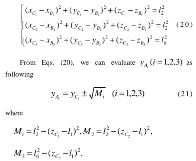
, the parallel singularity trajectory can be obtained, as shown in Fig. 7. Among them, the green part is the non-singularity workspace, and the red part is the singularity area, which indicates that there is a large non-singularity area inside the workspace. Fig. 8 is the projection view of the workspace in the XOZ and YOZ directions.

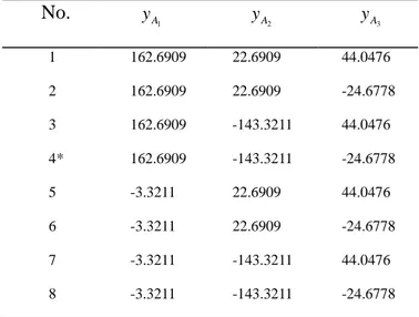
FIGURE 7 WORKSPACE AND THE PARALLEL SINGULARITY SITUATION

(A) XOZ PROJECTION (B) YOZ PROJECTION FIGURE 8 PROJECTION VIEW OF THE WORKSPACE IN

THE XOZ AND YOZ DIRECTION

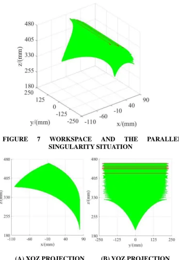
Fig. 9 shows four X-Y cross-sections in the Z direction of the workspace, which shows that the singularity and non-singularity workspace in each section also change with the change of Z value.

(12)

(A) Z=300 (B) Z=350

(C) Z=400 (D) Z=450

FIGURE 9 DIFFERENT X-Y CROSS-SECTIONS IN THE WORKSPACE

CONCLUSIONS

The new 3-translational (3T) PM proposed in this paper has three advantages: (1) it is only composed of three actuated prismatic joints and other passive revolute joints, which is easy to be manufactured and assembled; (2) it has analytical direct position solutions, which brings the great convenience to error analysis, dimensional synthesis, stiffness and dynamics research; and (3) it has partial input-output motion decoupling, which is very beneficial to the trajectory planning and motion control of the PM.

According to the kinematics modeling principle proposed by the author based on the single-opened-chains method, in the first loop with positive constraint, the set one virtual variable



can be directly obtained by the special geometric constraint condition that the output link of the first loop always maintains the horizontal position (the condition is provided by the second loop with negative constraint). Therefore, the entire analytical position solutions are obtained without solving the virtual variable



by the geometric constraint equation in the second loop with negative constraint. This is the advantage of the topology of the PM being different from other PM, and it has analytical direct solutions. The method has clear physical

meaning and simple calculation.

Based on the inverse solution, the conditions and locations of the three types of singularity configurations of the PM are obtained, and the size of the workspace of the PM and its parallel singularity area are given. The work of this paper lays the foundation for the stiffness, trajectory planning, motion control, dynamics analysis and prototype design of the PM.

ACKNOWLEDGMENTS:

This research is sponsored by the NSFC (Grant No.51475050 and No.51375062) and Jiangsu Key Development Project (No.BE2015043).

REFERENCES

[1] Clavel R. A Fast Robot with Parallel Geometry [C]. Proceeding of the 18th Int. Symposium on Industrial Robots. 1988: 91-100.

[2] Stock M, Miller K. Optimal Kinematic Design of Spatial Parallel Manipulators: Application to Linear Delta Robot [J]. Journal of Mechanical Design, 2003, 125 (2): 292-301.

[3] Bouri M, Clavel R. The Linear Delta: Developments and Applications [C]. Robotics. VDE, 2010: 1-8.

[4] Kelaiaia R, Company O, Zaatri A. Multiobjective optimization of a linear Delta parallel robot [J]. Mechanism & Machine Theory, 2012, 50 (2): 159–178.

[5] Tsai L. W., G. C. Walsh and R. E. Stamper, “Kinematics of a Novel Three DoF Translational Platform,” IEEE International Conference on Robotics and Automation, Minneapolis, MN 3446-3451 (1996).

[6] Tsai L. W and S. Joshi, “Kinematics and optimization of a spatial 3-UPU parallel manipulator,” ASME, J.Mech. Des. 122, 439-446 (2000).

[7] Zhao T., Huang Z., Kinematics analysis of a three dimensional mobile parallel platform mechanism. China Mechanical Engineering, 2001, 12 (6): 612-616.

(13)

[8] Yin X., Ma L.,Workspace Analysis of 3-DOF translational 3-RRC Parallel Mechanism [J]. China Mechanical Engineering, 2003, 14 (18): 1531-1533.

[9] X. Kong and C. M. Gosselin, “Kinematics and singularity analysis of a novel type of 3-CRR 3-DOFtranslational parallel manipulator,” Int. J. Robot. Res. 21, 791-798 (2002).

[10] Li S, Huang Z, Zuo R. Kinematics of a Special 3-DOF 3-UPU Parallel Manipulator [C] ASME 2002 International Design Engineering Technical Conferences and Computers and Information in Engineering Conference. 2002: 1035-1040.

[11] Li S, Huang Z. Kinematic characteristics of a special 3-UPU parallel platform manipulator [J]. China Mechanical Engineering, 2005, 18 (3): 376-381.

[12] Yu J., Zhao T., Bi S., Comprehensive Research on 3-DOF Translational Parallel Mechanism. Progress in Natural Science, 2003, 13 (8): 843-849.

[13] Lu J, Gao G., Motion and Workspace Analysis of a Novel 3-Translational Parallel Mechanism [J]. Mechinery Design & Manufacture, 2007,11 (11): 163-165.

[14] Yang T., Topology Structure Design of Robot Mechanisms [M]. China Machine Press, 2004.

[15] Yang T., Liu A., Luo Y.,et.al，Theory and Application of Robot Mechanism Topology [M]. Science Press, 2012.

[16] Yang T., Liu A., Shen H. et.al, Topology Design of Robot Mechanism [M]. Springer, 2018.

[17] Yang T., Liu A., Shen H. et.al, Composition Principle Based on Single-Open-Chain Unit for General Spatial Mechanisms and Its Application,Journal of Mechanisms and Robotics，OCTOBER 2018, Vol. 10 / 051005-1~051005-16

[18] Zhao Y. Dimensional synthesis of a three translational degrees of freedom parallel robot while considering kinematic anisotropic property [J]. Robotics and Computer-Integrated Manufacturing, 2013, 29 (1): 169-179.

[19] Zeng Q, Ehmann K F, Cao J. Tri-pyramid Robot: Design and

kinematic analysis of a 3-DOF translational parallel manipulator [M]. Pergamon Press, Inc. 2014.

[20] Zeng Q , Ehmann K F, Jian C. Tri-pyramid Robot: stiffness modeling of a 3-DOF translational parallel manipulator [J]. Robotica, 2016, 34 (2): 383-402.

[21] Lee S, Zeng Q, Ehmann K F. Error modeling for sensitivity analysis and calibration of the tri-pyramid parallel robot [J]. International Journal of Advanced Manufacturing Technology, 2017 (5): 1-14.

[22] PRAUSE I, CHARAF E. Comparison of Parallel Kinematic Machines with Three Translational Degrees of Freedom and Linear Act u at i o n [ J] . C H I N E S E J O U R N A L O F M E C H AN I C A L ENGINEERING, Vol. 28, No.4, 2015.

[23] Mahmood M, Mostafa T. Kinematic Analysis and Design of a 3-DOF Translational Parallel Robot [J]. International Journal of Automation and Computing, 14 (4), August 2017, 432-441.

[24] Shen H., Xiong K., Meng Q., Kinematic decoupling design method and application of parallel mechanism [J] .Transactions of The Chinese Society of Agricultural Machinery, 2016, 47 (6): 348-356.