HAL Id: hal-00840393
https://hal.archives-ouvertes.fr/hal-00840393
Submitted on 4 Jul 2013
HAL is a multi-disciplinary open access
archive for the deposit and dissemination of
sci-entific research documents, whether they are
pub-lished or not. The documents may come from
teaching and research institutions in France or
abroad, or from public or private research centers.
L’archive ouverte pluridisciplinaire HAL, est
destinée au dépôt et à la diffusion de documents
scientifiques de niveau recherche, publiés ou non,
émanant des établissements d’enseignement et de
recherche français ou étrangers, des laboratoires
publics ou privés.
Rouwaida Abdallah, Arnaud Gotlieb, Loïc Hélouët, Claude Jard
To cite this version:
Rouwaida Abdallah, Arnaud Gotlieb, Loïc Hélouët, Claude Jard. Scenario Realizability with
Con-straint Optimization. FASE 2013, Mar 2013, Rome, France. pp.194-209. �hal-00840393�
optimization
?Rouwaida Abdallah1, Arnaud Gotlieb2, Lo¨ıc H´elou¨et3,Claude Jard4
1
ENS Cachan (antenne de Bretagne),2
SIMULA, Norway,3 INRIA Rennes, 4 Universit´e de Nantes [email protected],{arnaud.gotlieb,loic.helouet}@inria.fr, [email protected]
Abstract. This work considers implementation of requirements expressed as High-level Message Sequence Charts (HMSCs).All HMSCs are not implementable, but a particular subclass called local HMSCs can be im-plemented using a simple projection operation. This paper proposes a new technique to transform an arbitrary HMSC specification into a local HMSC, hence allowing implementation. We show that this transforma-tion can be automated as a constraint optimizatransforma-tion problem. The impact of modifications brought to the original specification can be minimized w.r.t. a cost function. The approach was evaluated on a large number of randomly generated HMSCs.The results show an average runtime of a few seconds, which demonstrates applicability of the technique.
1
Introduction
In many system development methodologies, the user first specifies the system’s use cases. Some specific instantiations of each use case are then aggregated and described using a formal language. In the context of distributed applications we consider, high-level message sequence charts (HMSCs) and their variants are very popular. They are standardized by the ITU [9], and a variant called sequence diagrams is part of the UML notation. HMSCs are particularly useful in early stages of development to describe interactions between processes (or objects).
In a later modeling step of the development, state diagrams (i.e. automata) prescribe a behavior for each of the processes. Finally, the processes are im-plemented as code in a specific programming language. Parts of this design flow can be automated. We consider here the automated transformation of HMSCs into the model of communicating finite state machines (CFSMs), which will serve as a skeleton for the development of future code. The produced CFSM model is called the implementation of the HMSC.
However, HMSCs are not always implementable. HMSCs are automata la-belled by communication patterns involving several processes. When a choice between two patterns exists, all processes are assumed to behave according to the same pattern. However, in CFSM, processes are independent, and the global
?Work supported by the ANR IMPRO(ANR-2010-BLAN-0317) of the French
coordination of HMSCs might be lost in implementations when the HMSC is not local, that is contains a choice between two patterns in which the first events to be executed occur on distinct processes. Implementations of non-local HMSCs may exhibit more behaviors than the original specification, and can even dead-lock. Non-local HMSCs can be considered as too incomplete or too abstract to be implemented. On the other hand, local HMSCs avoid the global coordination problem, and can always be implemented.
This paper proposes to extend the possibility of automated production of CFSMs by the use of a localization procedure that transforms any non-local HMSC into a local one. It guarantees that every choice in the transformed local HMSC has a leader process, which chooses one scenario and communicates its choices to the other processes. This can be achieved by adding new messages and processes in scenarios. Trivial but uninteresting solutions to the localization problem exist (force all processes to participate in all interactions, and choose the same leader for every choice). We are thus interested in finding solutions with the minimal number of added messages because they correspond to the less disturbing transformation of the specification. In our work, we propose to address the localization problem with a constraint optimization technique. We build a constraint model where variables represent leader processes or processes contributing to a scenario and constraints capture the localization properties of HMSCs. A cost function is then proposed to minimize the number of added messages.The experiments we ran on a large class of randomly generated HMSCs show that localization takes in general a few seconds on ordinary machines.
Several work address automatic synthesis from scenario models. We refer interested reader to [10] for a survey on synthesis algorithms. The question of whether an HMSC specification can be implemented by an equivalent CFSM was shown undecidable in general [2, 11], so the key issue is to rely on imple-mentable classes of HMSCs. Several CFSM implementation techniques have been proposed for local HMSCs [7, 8, 1], or regular HMSC [3]. A variant of HMSCs, where communication patterns label shared high-level actions of a network of automata is translated to Petri nets in [14]. Up to our knowledge, no algorithm was proposed so far to transform non-local specifications into local ones.
This paper is organized as follows: Section 2 gives the basic formal defini-tions on HMSCs. Section 3 defines localization of HMSCs. Section 4 proposes an encoding of localization as a constraint optimization problem, and shows the correctness of the approach. Section 5 evaluates the performance of our local-ization procedure with an experimentation, and comments the results.Section 6 concludes this work.For space reasons, proof of theorems are omitted, but can be found in a full version available at: http://hal.inria.fr/hal-00769656.
2
Basic definitions
Message Sequence Charts (MSCs for short) describe the behavior of entities of a system called instances. It is frequently assumed that instances represent pro-cesses of a distributed system. MSCs have a graphical and textual notation, but are also equipped with a standardized semantics [13]. The language is composed
of two kinds of diagrams. At the lowest level, basic MSCs (or bMSCs for short) describe interactions among instances. The communications are asynchronous. A second layer of formalism, namely High-level MSCs (HMSCs for short), is used to compose these basic diagrams. Roughly speaking, an HMSC is an automa-ton which transitions are labeled by bMSCs, or by references to other HMSCs. However, in the paper, we will consider without loss of generality that our spec-ifications are given by only two layers of formalism: a set of bMSCs, and an HMSC with transitions labeled by these bMSCs.
Definition 1 (bMSCs). A bMSC defined over a set of instances P is a tuple M = (E, , λ, φ, µ) where E is a finite set of events, φ : E −! P localizes each event on one instance. λ : E −! ⌃ is a labeling function that associates a type of action to each event. The label attached to a sending event is of the form p!q(m) denoting a sending of message m from p to q. Similarly, the label attached to a reception is of the form p?q(m) denoting a reception on p of a message m sent by q. Last, events labeled by p(a) represent a local action a of process p. Labeling defines a partition of E into sets of sending events, reception events, and local actions, respectively denoted by ES,ER and EL. µ : ES −! ER is a
bijection that maps sending events with a corresponding reception. If µ(e) = f , then λ(e) = p!q(m) for some p, q, m and λ(f ) = q?p(m). ✓ E2 is a partial
order relation called the causal order.
It is required that events of the same instance are totally ordered: 8(e1, e2) 2
E2, φ(e
1) = φ(e2) =) (e1 e2) _ (e2 e1). For an instance p, let us call pthis
total order. must also reflect the causality induced by the message exchanges, i.e. = (S
p2P
p[ µ)⇤. The graphical representation of bMSCs defines instances
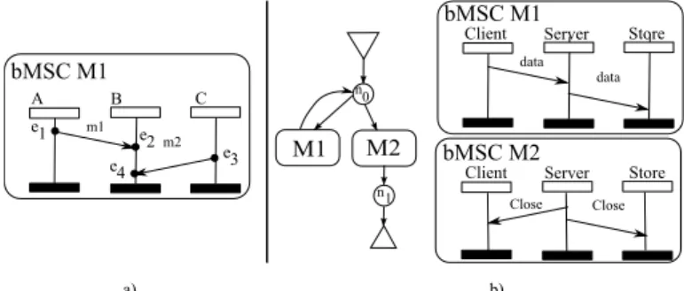
as vertical lines. All events executed by an instance are ordered from top to bottom. Horizontal arrows represent messages from one instance to another. Figure 1-a) is an example of bMSC, with three instances A, B, C, exchanging two messages m1,m2. The events e1 and e3 are sending events, and the events
e2 and e4 are the corresponding receptions.
Fig. 1: An example bMSC and an example HMSC
For a bMSC M , we will denote by min(M ) = {e 2 E | 8e0 2 E, e0 e )
be the first event executed in M . An instance is called minimal if it carries a minimal event. A minimal instance (i.e. a process in φ(min(M ))) is an instance that can execute the first events in M . In other words, it can decide to start executing M rather than another scenario. A bMSC is local if it has a single minimal instance.
The semantics of a bMSC M is denoted by Lin(M ), and defined as the linearizations of M , that is sequences of actions that follow the causal ordering imposed by M . We refer interested readers to the full version for details. Basic MSCs only describe finite interactions.They have been extended with HMSCs to allow iteration, choices, and parallel composition.For simplicity, we restrict to HMSCs without parallel frames, and with only one hierarchical level. With these assumptions, HMSCs can be seen as automata labeled by bMSCs. Definition 2 (HMSCs). An HMSC is a graph H = (I, N, !, M, n0), where
I is a finite set of instances, N is a finite set of nodes, n0 2 N is the initial
node of H, M is a finite set of bMSCs, defined over disjoint set of events, and !✓ N ⇥ M ⇥ N is the transition relation.
In the rest of the paper, we consider without loss of generality that all nodes, except possibly the initial node and sink nodes, are choice nodes ( i.e. have several successors by the transition relation). We will denote by Pi the set of active
processes that interacts within a bMSC Mi2 M. HMSCs also have a graphical
representation: Nodes are represented by circles, references to bMSCs by boxes. The initial node of an HMSC is connected to a downward pointing triangle, and final nodes to an upward pointing triangle. The example of Figure 1-b) shows an example of HMSC, with two nodes n0, n1. Intuitively, this HMSC depicts a
protocol in which three processes exchange data, before closing a session. This very simple HMSC allows for the definition of iterations: bMSC M 1 can be repeated several times before the execution of bMSC M 2. Note however that even if a bMSC M 1 is seen before a bMSC M 2 along a path of H, this does not mean that all events of M 1 are executed before M 2 starts. The semantics of an HMSC is defined using sequential composition of bMSCs.
We do not define formally sequential composition of bMSCs, and refer inter-ested readers to thefull version. Intuitively, composing sequentially two bMSCs M1 and M2 consists in drawing M2 below M1 to obtain a new bMSC. The
se-quential composition is denoted by M1◦ M2. From this intuitive definition, we
can immediately notice that if some events in min(M2) are located on processes
that do not appear in M1, then they are also minimal in M1◦ M2. This raises
two important remarks: first, executing M1◦ M2 does not mean executing M1
then M2, but rather executing the bMSC obtained by concatenation of M1 and
M2, and then minimal events in a concatenation M1◦ . . . Mk are not all located
in M1.
A path of H is a sequence of transitions ⇢ = (n1, M1, n01) . . . (nk, M1, n0k) such
that n0
i = ni+1. A path is called initial if it starts from node n0. Each path
⇢ = (n1, M1, n01) . . . (nk, M1, n0k) defines a unique bMSC M⇢= M1◦ M2· · · ◦ Mk.
bMSCs M⇢such that ⇢ is an initial path of H. With this semantics, HMSCs are
very expressive. They are more expressive than finite state machines (they can describe non-regular behaviors, as shown by the example of Figure 1-b)).
The implementation problem consists in building a set of communicating machines A = {A1, . . . Ak} (one frequently uses as model the
Communicat-ing Finite State Machines (CFSM) proposed by [5]) such that L(A) = L(H). It is frequently assumed that these communicating machines are obtained by simple projection of the original HMSC on each instance. The realizability prob-lem consists in deciding whether there exists an impprob-lementation A such that L(A) = L(H). Realizability was shown undecidable in general [2, 11]. On the other hand, several papers have shown automatic and correct synthesis tech-niques for subclasses of HMSCs [7, 8, 3, 1]. The largest known subclass is that of local HMSCs [4]. These results clearly show that automatic implementation can not apply in general to HMSC. However, non-local HMSCs can be considered as too abstract to be implemented, and need some refinement to be implementable. In the rest of the paper, we hence focus on a transformation mechanism that transforms an arbitrary HMSC into a local (and hence implementable) HMSC.
Let us consider the example of Figure 1-b). Node n0is a choice node,
depict-ing a choice between two behaviors: either continue to send data (bMSC M1), or
close the data transmission (bMSC M2). However, the deciding instance in M1
is the Client, while the deciding instance in M2 is the Server. At
implementa-tion time, this may result in a situaimplementa-tion where Client decides to perform M1and
Server decide concurrently to perform M2, leading to a deadlock of the protocol.
Such situation is called a non-local choice, and obviously causes implementation problems. It is then safer to implement HMSCs without non-local choices. At each choice, a single deciding instance chooses to perform one scenario, and all other non-deciding instances must conform to this choice.
Definition 3 (Local choice node). Let H = (I, N, !, M, n0) be an HMSC.
Let c 2 N , c is a local choice if and only if for every pair of (non necessarily distinct) paths ⇢ = (c, M1, n1)(n1, M2, n2) . . . (nk, Mk, nk+1) and
⇢0= (c, M0
1, n01)(n01, M20, n02) . . . (n0q, Mk0, n 0
q+1) there is a single minimal instance
in M⇢ and in M⇢0
(i.e. φ(min(M⇢)) = φ(min(M⇢0
)) and |φ(min(M⇢))| = 1).
H is called a local HMSC if all its nodes are local.
Due to the semantics of concatenation, non-locality can not be checked on a pair of bMSCs leaving node c, but has to be checked for pairs of paths. Intuitively, locality of an HMSC H guarantees that every choice in H is controlled by a unique deciding instance. Checking whether an HMSC is local is decidable [8], and one can show that this question is in co-NP [1]. It was shown in [7] that for a local HMSC H = (I, N, !, M, n0), if for every Mi 2 M we have Pi= I,
then there exists a CFSM A such that L(A) = L(H).A solution was proposed to leverage this restriction in [1], and allow implementation of any local HMSC. An immediate question that arises is: how to implement non-local HMSCs? In the rest of the paper, we propose a solution that transforms any non-local HMSC into a local one, hence allowing its implementation. This results in slight
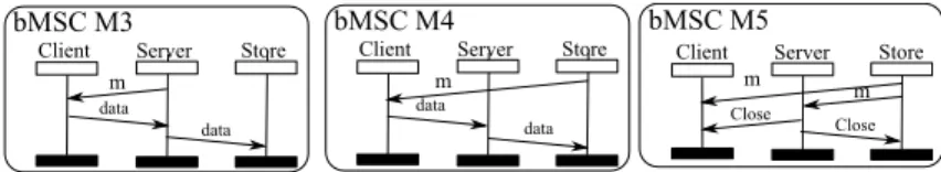
modifications of the original specification. We allow additional active instances and new messages in bMSCs, but do not change the structure of the HMSC. Consider the example of Figure 1-b). Replacing M1by the bMSC M3of Figure 2
solves the non-local choice problem. Similarly, replacing M1and M2respectively
by M4 and M5solves the the non-locality problem, but needs more messages.
Fig. 2: Solutions for localization of HMSC in Figure 1-b)
This example raises several remarks. First, the proposed transformations are purely syntactic, and modifying the set of minimal instances does not always produce a meaningful specification. For this reason, the examples exhibit changes involving a single message type m. A meaning for additional message has to be chosen adequately by the designer once an HMSC is localized. The second remark is that there are several possibilities for localization. The first solution proposed adds one message in bMSC M1 to obtain M3. The second solution
adds one message to M1 and two to M2, and one can notice that in M5, the
message between Store and Client is useless. Indeed, there exists an infinite number of transformations to localize an HMSC. This calls for the following solutions: we want to restrict to cheapest solutions (for instance solutions with a minimal number of added messages). As we will show later, once a deciding instance for a choice is fixed, one can compute the minimal number of messages needed to localize this choice. As a consequence, the solutions to a localization problem can be given in terms of choosing a deciding instances at each choice, and instances participating to bMSCs. Then, the localization can be easily tuned using different cost functions.
3
Localization of HMSCs
In this section, we show how to transform a non-local HMSC into a local one. This procedure called localization consists in choosing a single deciding instance for each bMSC M in the HMSC so that all choices become local, and then ensure that all other instances execute their minimal events only after the first event (the choice) of the deciding instance. This is done by adding messages, as in the examples of Fig. 2.
Definition 4. Let M be a bMSC over a set of events E and processes P , with minimal events e1, . . . , ek. A localized extension of M is a bMSC M0 over a
set of events E0 ◆ E and over P0 ◆ P , such that there exists a minimal event
emin 2 E0 and for every e f 2 E, we have e 0 f . The unique minimal
instance in a localized bMSC M is called the leader of M .
Note that as there exists an infinite number of extensions for a bMSC M , choosing extensions that are as close as possible to the original model is desirable.
The impact of localization can be simply measured as the number of added messages. A more generic approach is to associate a cost to communications between processes, and to choose extensions with minimal cost. This makes sense, as for instance the cost and delays for communications via satellite are higher than with ground networks. Similarly, the configuration of a system may prevent two processes p and q from exchanging messages. To avoid solutions with communications between p and q, one can design a cost function that associates a redhibitory (or even infinite) cost to such communications.
For a given bMSC M with k minimal events, there exists a localized extension over the same set of processes that contains exactly k − 1 additional messages. This localized extension is built when one picks up a deciding instance among the d the minimal instances of M , and create causal dependencies from the minimal event on instance d to all other minimal events with additional messages. Only k − 1 messages are necessary in this case, regardless to their respective ordering and place of insertion in the orginal bMSC. Another possibility is to pick up another non-minimal process among those of M that do not carry a minimal event as a leader, or even add a new process to M . In such cases, a localized extension can always be built with exactly k additional messages.
Localization of HMSCs is more complex than localization of bMSCs. For each non-local choice c, we have to ensure that every branch leaving c has the same leader. Hence, this is not a property purely local to bMSCs. As for bMSCs, we can define a notion of localized extension of a HMSC as follows:
Definition 5. Let H = (I, N, −!, M, n0) be an HMSC. H0= (I, N, −!0, M0, n0)
is a localized extension of H iff there is a bijection f : M ! M0 such that
8M 2 M, f (M ) is a localized extension of M , −!0= f (−!), and H0 is a local
HMSC.
Localizing an HMSC H consists in finding M0 and the bijection f . As
men-tionned above, as there exists a (potentially) infinite number of solutions, we consider the solutions with the smallest number of changes to the original model. We propose to address this problem with a cost function F that evaluates the cost of each possible transformation of H. The goal of our localization algorithm is thus to minimize F. For the sake of simplicity in this paper, F counts the total number of messages and instances added in M0. As localization transforms M
into M0, F is defined as a sum of individual costs of modifications. Formally,
F(H, H0), X
M2M
cM,f(M )
where cM,M0 is the individual cost to transform M into M0. When H is clear from
the context, we will write F(H0) instead of F(H, H0). Let M
i2 M be a bMSC,
M0
i = f (Mi), IMi, IMi0 be the set of instances in Mi and M
0
i. Let k = |min(Mi)|
be the number of minimal instances in Mi, l be the leader instance of Mi0, and
x = |IM0
i| − |IMi| be the number of new instances in Mi. We choose a constant
✓ 2 [0, 1] and define the cost cMi,Mi0 for transforming Mi into M
0 i as follows: cMi,Mi0 , ( x ⇤ ✓ + (k + x − 1) ⇤ (1 − ✓) if l 2 φ(min(Mi)) or l /2 IMi x ⇤ ✓ + (k + x) ⇤ (1 − ✓) otherwise
Intuitively, cMi,Mi0 is the barycenter between the number of added messages,
and the number of added instances, weighted by ✓. We already know that the number of messages to add is at most k − 1 if we have k minimal instances. Adding x instances to Mihence yields adding (k + x − 1) messages if l is chosen
among the minimal instances of Mior among the new instances. Similarly, if the
leader instance is chosen among instances that are not minimal w.r.t the causal ordering, one need to add k + x messages to localize Mi. The value ✓ is chosen to
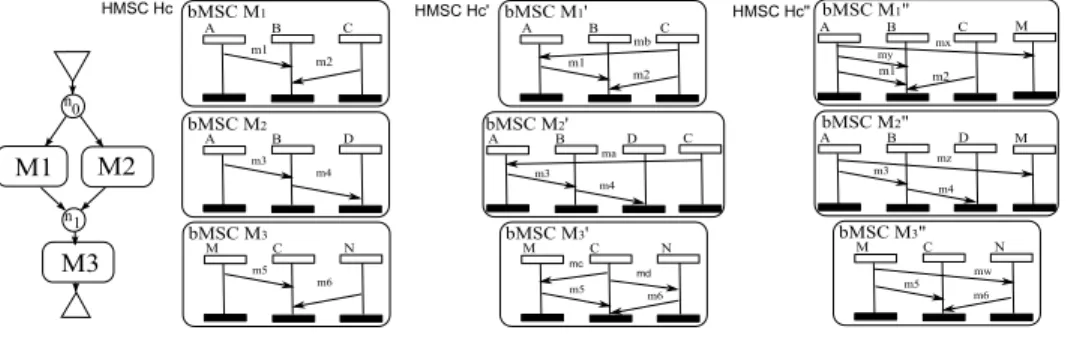
penalize more the number of added processes or the number of added messages. Let us illustrate the computation of F on an example. Let Hcbe the HMSC
on the right of Figure 3, and let H0
c be a localization of Hc. As mentionned
above, F(Hc, Hc0) = cM1,M10 + cM2,M20 + cM3,M30. The leader of M
0
1 is C and, as
C 2 min(M1) = {A, C}, then cM0
1 = 1 − ✓ (there is a single message added
in M0
1). The leader of M20 is also C, but C is not an instance of M2, so cM0 2 =
✓ +(1−✓) = 1 (there is a single message and a single instance added in M0 2). The
leader of M0
3 is again C. As C is an instance of M3 but not a minimal instance
we have cM0
3 = 2 ⇤ (1 − ✓). As a result, F(Hc, H
0
c) = 1 − ✓ + 1 + 2 ⇤ (1 − ✓) =
4 − 3 ⇤ ✓. One can easily notice that H0
cis local. If we compare Hc with another
localization Hc00, depicted at the right of Figure 3, we get that cM1,M100 = 1,
cM2,M200 = ✓, cM3,M300 = 0 and finally, F(Hc, H
00
c) = 1 + ✓. If ✓ = 0.5 then
F(Hc, Hc00) < F(Hc, Hc0) and thus, localization Hc00 shoud be preferred to Hc0.
On the other hand, if ✓ = 1.0, then H0
c should be preferred. This example shows
that the cost funtion influences the choice of a particular localization solution.
Fig. 3: localizing the HMSC Hc
The cost function F defined above that counts the number of new messages and processes in bMSCs is only an example, and other functions can be consid-ered. For instance, a cost function can consider concurrency among events as an important property to preserve, and thus impose a penality everytime a pair of events e, e0 is causally ordered in f (M ), but not in M .
Note also that several localization solutions can have the same cost. For in-stance, if F is used, the order in which messages are exchanged to obtain localized bMSCs is ignored. Considering that the cost function is influenced only by the number of added messages and added processes, we define F(H, {(IM0, lM0)}M2M)
has lM0 as leader for every M 2 M. The localization problem can be formally
defined as follows:
Definition 6. Let H = (I, N, −!, M, n0) be a non-local HMSC, and F be a
cost function. The localization problem for H, F consists in returning solu-tions s1, . . . , sk, where each si is of the form si = {(IM0 , l0M)}M2M such that
F(H, {(IM0, lM0)}M2M) is minimal, and where for each M 2 M, IM0 ✓ I is a
set of instances appearing in M0 = f (M ) and l
M02 IM0 is the leader of M0.
4
Localization as a constraint optimization problem
This section explains how a finite domain constraint optimization model is con-structed from a given HMSC, to minimize the cost of the localization.
4.1 Constraint solving over finite domains
A constraint solving problem is composed of a finite set of variables X1, . . . , Xn,
where each variable Xi ranges over a finite domain, noted D(Xi). An
assign-ment of a variable is a choice of a value from its domain. A set of constraints C1, . . . , Cm is defined over the variables and the goal in a constraint solving
problem is to find solutions, i.e., assignments for all variables, that satisfy all constraints. A constraint solving problem is satisfiable if it allows at least one solution. When a cost function F is associated to each assignment, the problem becomes a constraint optimization problem (COP) where the goal is to find a solution that optimizes the cost. Such a solution is called an optimal solution.
Constraint solving frequently uses filtering and propagation. Roughly speak-ing, the underlying idea is to consider each constraint in isolation, as a filter over the domains. Filtering a domain means eliminating inconsistent values w.r.t. a given a constraint. For example, if D(X) = {1, 3, 4} and D(Y ) = {2, 3, 4, 5}, the constraint X > Y filters D(X) to {3, 4} and D(Y ) to {2, 3}. Once a reduction is performed on the domain of a variable, constraint propagation awakes the other constraints that hold on this variable, in order to propagate the reduction. Con-straint propagation is a polynomial process: it takes O(n ⇤ m ⇤ d) where n is the number of variables, m is the number of constraints and d is the maximum number of possible values in the domains.
Constraint propagation and filtering alone do not guarantee satisfiability, and just prune the domains without trying to instantiate variables. For example, con-sidering the constraint system shown above, the constraint X > Y prunes the domains D(X) to {3, 4} and D(Y ) to {2, 3} but (3, 3) is not a solution of the constraint. The constraint system may even be unsatisfiable, while constraint propagation and filtering does not detect it (i.e., they ensure only partial sat-isfiability). Hence, an additional step called labeling search is needed to exhibit solutions. Labeling search consists in exploring the search space composed of the domains of uninstantiated variables. Interestingly, a labeling procedure can awake constraint propagation and filtering, allowing an early pruning of the search space. In the previous example, if X is labeled by 3 then the constraint
X > Y is awoken and automatically reduce the domain of Y to {2}. A labeling search procedure is complete when the whole search space is explored. Complete labeling search can eventually determine satisfiability (or unsatisfiability) of a constraint solving problem over finite domains. However, it is an exponential procedure in the worst case. This is not surprising as determining satisfiability of a constraint problem over finite domains is NP-hard [15].
During labeling search, when a solution s is found, the value m = F(s) of the cost function can be recorded, and backtracking can then be enforced by adding the constraint F(...) < m to the set of constraints (or F(...) m if one wants to explore all optimal solutions). If another solution is found, then the cost function F will necessarily have a cost smaller than m. This procedure, called branch&bound [12], can be controlled by a timeout that interrupts the search when a given time threshold is reached. Of course, the current value of F in this case may not be a global minimum, but it is already an interesting value for the cost function, something that we call a quasi-optimum. For localization of HMSCs, selecting the local HMSC with the smallest cost is desirable but not always essential. On the other hand, mastering the time spent for localization is essential to scale to real-size problems.
4.2 From HMSC to COP
Variables. Localizing an HMSC H consists in selecting a set of participating instances and a minimal process for each bMSC appearing in H, such that every choice in the HMSC becomes a local choice. As this selection is not unique, we use constraint optimization techniques to provide characteristics of localized HMSCs with minimal cost. We propose to transform any HMSC into a constraint optimization problem, as follows: a couple of variables (Xi, Yi) is associated to
each bMSC Mi 2 M, where Xi represents the set of instances chosen for the
bMSC f (Mi), and Yi represents the leader in f (Mi). If I is the set of instances
of H, every Xi takes its possible values in 2I while Yi takes a value in I.
Constraints. Our constraint model is composed of domain, equality and inclusion constraints. Domain constraints, noted DOM , are used to specify the domains of Xi and Yi. Obviously, if a bMSC Mi is defined over a set of
pro-cesses Pi, we have Pi ✓ Xi ✓ I. Equality constraints, noted EQU , enforce the
locality property. For two bMSCs Mi, Mj such that there exists two transitions
(n, Mi, n1) and (n, Mj, n2) in ! originating from the same node n, f (Mi) and
f (Mj) must have the same leader, i.e., Yi = Yj. We write Mi⌦ Mj, when such
choice between Mi and Mj exists in H. Locality of HMSCs is also enforced by
using inclusion constraints, noted IN CL. Let Mi, Mj 2 M be two bMSCs. We
write Mi. Mj when there exists a path (n, Mi, n0)(n0, Mj, n00), i.e., when Mi is
the predecessor of Mj in H. In such case, in any localization of H, the
mini-mal instance of f (Mj), represented by variable Yj, must appear in the set of
instances of f (Mi), represented by variable Xi. In our constraint model, this
is expressed by the constraint Yj 2 Xi. Similarly, the leader of a bMSC in the
localized solution can only be one of its instances, so we have Yi2 Xi for every
It is worth noticing that the localization problem is always satisfiable, as there exists at least one trivial solution: select an instance in I as leader for all bMSCs, then add this instance if needed to every bMSC, and messages from this instance to all other instances. However, this trivial and uninteresting solution is not necessarily minimal w.r.t. the chosen cost function. We can now prove that our approach is sound and complete by considering the following definition: Definition 7. Let H = (I, N, !, M, n0) be an HMSC, the constraint
optimiza-tion model associated to H is CPH = (X , Y, C) where X = {X1, . . . , X|M|}
associates a variable to the set of instances appearing in each bMSC of f (M), Y = {Y1, . . . , Y|M|} associates a variable to the leader selected for each bMSC of
f (M), and C = DOM [ EQU [ IN CL is a set of constraints defined as follows:
– DOM = V i21...|M| Xi2 2I ^ Pi✓ Xi^ Yi2 I ; – EQU = V Mi,Mj|Mi⌦Mj Yi= Yj – IN CL = V Mi,Mj|Mi.Mj Yj2 Xi^ V i21...|M| Yi2 Xi
Then, solving the localization problem for an HMSC H amounts to find an optimal solution for CPH, w.r.t. cost function F. We have:
Theorem 1. Computing solutions for a localization problem using an optimal solution search for the corresponding COP is a sound and complete algorithm.
This result is not really surprising, as CPH represents what is needed for an
HMSC to become local.A proof of this theorem can be found in the full version of the paper.
5
Implementation and experimental results
To evaluate the approach proposed in the paper, we implemented a systematic transformation from HMSC descriptions to COPs and conducted an experimen-tal analysis over a large number of randomly generated HSMCs. Our implemen-tation contains three main components G, A and S and is described in Figure 4. G is a random HMSC generator, A is an analyzer that transforms a localization problem for a given HMSC into a COP , as described in the previous section. Finally S is a constraint optimization solver: we used the clpfd library of SIC-Stus Prolog [6]. The generator G takes an expected number of distinct HMSCs to generate (nbH), a number of bMSCs in each HMSC(nbB), and a number of active processes in each HMSC (nbP ) as inputs. As output, it produces an xml file containing nbH randomly generated HMSCs.
The analyser A takes T h, the parameter ✓ of the cost function F, a set of heuristics R, and a sequence of time-out values T , as inputs. These values can be considered as internal parameters for the constraint optimization solver: They allow us to evaluate different strategies. In the experiments, we considered sev-eral labeling heuristics to choose the variable and the value to enumerate first, e.g., leftmost, first-fail, ffc, step or bisect. Leftmost is a variable-choice heuristic
Fig. 4: The input and outputs of the generator, the analyser and the solver. that selects the first unassigned variable from a statically ordered list. First-fail is a dynamic variable-choice heuristic that selects first the variable with the current smallest domain. Ffc is an extension of first-fail that uses the number of constraints on a given variable as a tie-break when two variables have the same domain size. Step is choice-value heuristic that consists in traversing incre-mentally the variation domain of the current variable. Finally, bisect implements domain splitting which consists in dividing a domain into two subdomains and propagating the subdomain informations. For example, if x takes a value in an interval [a, b], then bisect will propagate first x 2 [a,a+b
2 ], and then x 2 [ a+b
2 , b]
upon backtracking. For each generated HMSC H and each heuristic hi2 R, the
analyser creates a prolog file that contains the corresponding COP. For efficiency reasons, a special attention has been paid to the encoding of variation domains and constraints. Subset domains were encoded using a binary representation and sets inclusion using efficient div/mod operations. The prolog file is then used as input of the solver. The sequence T represents the various instants at which the optimization process must temporarily stop, and returns the current value of the cost function. These values are quasi-optima, representing approximations of the global optimum. The combination between heuristics and time-out values is useful to compare different labeling strategies. Finally, the analyser A collects all the results returned by the solver with the time needed to provide a solution, and stores them for a systematic comparison.
The first step of the experiment consisted in a systematic evaluation of the performance of several heuristics to guide the solver. During this step, we con-sidered several heuristics and time-outs. We do not report here all the results, but show only the results for one illustrative model. Figure 5 shows the time-aware minimization of the cost value with 12 different heuristics and time-outs between 1s and 14s for a chosen localization problem. Heuristics descriptions use the following syntax: [b — u] / [left — ff — ffc] / [bisect — step] / [XYC — YXC — CXY — CYX], where b and u stand resp. for bounded costs and unbounded costs. The heuristic bounded cost evaluates a lower bound on the cost of a solution that can be reached from a given state. Left, ff and ffc stand for a variable-choice heuristic, bisect and step stand for value-choice heuristic, and XYC, etc. stand for the static order in which variables are fed to the solver. Bold values indicate proved global minima, non-bold values indicate quasi-optima, – indicates absence of result in the given time contract.
In Figure 5, heuristics 3,9,10 give the best results. The series of experiment that we run shows that heuristics with an estimation of cost, and a static ordering of variable evaluations have the best performance. Overall, the heuristics number 10 combining bisect (domain splitting), left (static variable ordering), and a cost
heuristics \ runtime 1 s 2 s 3 s 4 s 5 s 6 s 7 s 12 s 13 s 14 s 0 u/left/step/XYC 23 23 22 22 22 22 19 19 19 19 1 u /left/step/YXC 19 19 2 b/left/step/XYC 19 19 3 b/left/step/YXC 19 4 b/left/step/CYX - - - 21 19 5 b/ff/step/XYC 22 19 19 19 19 19 6 b/ff/step/YXC 30 19 19 19 19 19 7 b/ff/step/CYX 30 19 19 19 19 19 8 b/ffc/step/CYX 27 22 19 19 19 19 19 9 b/left/bisect/XYC 19 10 b/left/bisect/YXC 19 11 b/left/bisect/CYX - - - - 21 19
Fig. 5: Comparing heuristics with one representative example.
evaluation exhibited the best results and was selected for the next steps of the experiment.
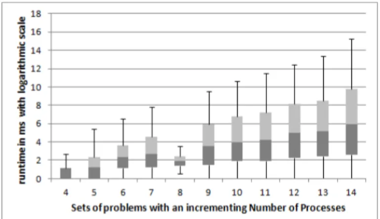
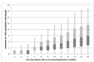
As next steps, we generated 11 groups of 100 random HMSCs, with 10 bM-SCs, which is a reasonably large number, according to the existing literature on HMSCs. We then let the number of processes grow from 4 to 14. We also generated 12 groups of 100 HMSCs, containing exactly 8 processes, and let the number of bMSCs grow from 4 to 15. The goal of these series of experiments was to evaluate the influence of both the number of processes and the number of bM-SCs on the runtime of our localization approach. We expected these parameters to influence the performance of localization, as increasing the number of bM-SCs increases the number of variables, and increasing the number of processes increases the size of variables’ domains. However, we have obtained solutions for all HMSCs, which allowed us to evaluate the impact of both parameters. The evaluation was performed on a machine equipped with INTEL P 9600 core2 Duo at 2, 53 Ghz, with 4Go of RAM. Results of both experiences are given in Fig-ures 6 and 7, using box-and-whiskers plots to show the statistical distribution of datasets.
Fig. 7: The influence of the number of bMSCs on the runtime execution Both plots use logarithmic scales to tackle the big variance between runtime measurements. As expected, the plots show exponential curves but the runtime for each group remains quite low. For randomly generated HMSCs of reasonable size (such as the ones found in the literature), our experimental results show that localization using constraint optimization takes a few minutes in the worst cases, and an average duration of a few seconds. Actually, even for the largest cases (15 bMSCs with 14 processes), the runtime of our localization approach did not exceed 40 minutes. Although solving COPs over finite domains is NP-hard [15], as examples of existing HMSCs usually contain less than 15 bMSCs, our local-ization process appears to be of practical interest. Our results are encouraging, and show that the approach is fast enough to be used in practice. However, they have been obtained on random instances only, and thus further experiments on non-random instances are necessary to confirm this judgment.
6
Conclusion and future work
This paper has proposed a sound and complete method to transform arbitrary HMSCs into implementable ones. Our approach transforms an HMSC in a con-straint optimization problem. The solution returned by a solver can be used to build an optimal localized version of the original specification, without changing the overall architecture of the HMSC. Once an HMSC is localized by addition of messages and processes in bMSCs, automatic implementation techniques can generate code for communicating processes. Our approach has been implemented and tested on a benchmark of 2300 randomly generated HMSCs. The experimen-tal results show that our approach is of practical interest: it usually takes less than a few minutes to localize an HMSC.
There are four foreseen extensions of this work. First, other cost functions can be considered as our approach does not depend on the choice of a particular cost function. For instance, we plan to study localization with functions that accounts for the cost of communications between instances. Second, we plan to
allow modifications of the HMSC, in addition to those brought to the bMSCs of the specification. Considering architectural constraints that disallow commu-nications between some processes is another challenging issue, as in this case existence of a solution is not guaranteed. Finally, noticing that localization is a rather syntactic procedure, the question of designating a process as a leader or adding messages should also be addressed in more semantics terms.
Further work also includes the experimentation of our approach on indus-trial case studies, to evaluate its performance on non-random HMSCs. We have started a collaboration with a company that develops communicating systems and wants to generate test cases based on requirement design. Our approach will be useful to derive automatically test cases from HMSCs that were designed without any requirement on implementability.
References
1. R. Abdallah, C. Jard, and L. H´elou¨et. Distributed implementation of message sequence charts. Software and Systems Modeling, to appear, 2013.
2. R. Alur, K. Etessami, and M. Yannakakis. Realizability and verification of msc graphs. In ICALP, pages 797–808, 2001.
3. N. Baudru and R. Morin. Synthesis of safe message-passing systems. In FSTTCS, pages 277–289, 2007.
4. H. Ben-Abdallah and S. Leue. Syntactic detection of process divergence and non-local choice in message sequence charts. In Proc. of TACAS’97, volume 1217 of
LNCS, pages 259 – 274, 1997.
5. D. Brand and P. Zafiropoulo. On communicating finite state machines. Technical Report 1053, IBM Zurich Research Lab., 1981.
6. M. Carlsson, G. Ottosson, and B. Carlson. An open-ended finite domain constraint solver. In PLILP, pages 191–206, 1997.
7. B. Genest, A. Muscholl, H. Seidl, and M. Zeitoun. Infinite-state high-level MSCs: Model-checking and realizability. Journal on Comp. and System Sciences, 72(4):617–647, 2006.
8. L. H´elou¨et and C. Jard. Conditions for synthesis of communicating automata from HMSCs. In Proc. of FMICS 2000, 2000.
9. ITU-T. Message sequence charts (msc). In ITU standard Z.120, 1999.
10. H. Liang, J. Dingel, and Z. Diskin. A comparative survey of scenario-based to state-based model synthesis approaches. In Proc. of SCESM ’06: the 2006 International
Workshop on Scenarios and State Machines: Models, Algorithms, and Tools, pages 5–12, 2006.
11. M. Lohrey. Realizability of high-level message sequence charts: closing the gaps.
Theoretical Computer Science, 309(1-3):529–554, 2003.
12. K. Marriott and P.J. Stuckey. Programming with Constraints: An Introduction. MIT Press, 1998.
13. M. Reniers and S. Mauw. High-level Message Sequence Charts. In SDL97: Time
for Testing - SDL, MSC and Trends, Proc. of the 8th SDL Forum, pages 291–306, 1997.
14. Abhik Roychoudhury and P. S. Thiagarajan. Communicating transaction pro-cesses. In ACSD 2003, pages 157–166. IEEE Computer Society, 2003.
15. P. Van Hentenryck, V.A. Saraswat, and Y. Deville. Design, implementation, and evaluation of the constraint language cc(fd). J. Log. Program., 37(1-3):139–164, 1998.