Resonant dynamics of Super-Earth systems

HAL Id: tel-02438364

https://tel.archives-ouvertes.fr/tel-02438364

Submitted on 14 Jan 2020

HAL is a multi-disciplinary open access

archive for the deposit and dissemination of

sci-entific research documents, whether they are

pub-lished or not. The documents may come from

teaching and research institutions in France or

abroad, or from public or private research centers.

L’archive ouverte pluridisciplinaire HAL, est

destinée au dépôt et à la diffusion de documents

scientifiques de niveau recherche, publiés ou non,

émanant des établissements d’enseignement et de

recherche français ou étrangers, des laboratoires

publics ou privés.

Resonant dynamics of Super-Earth systems

Gabriele Pichierri

To cite this version:

Gabriele Pichierri. Resonant dynamics of Super-Earth systems. Astrophysics [astro-ph]. Université

Côte d’Azur, 2019. English. �NNT : 2019AZUR4054�. �tel-02438364�

Dynamique r´esonante des syst`emes de Super-Terres

Gabriele PICHIERRI

Laboratoire J.-L. Lagrange (UMR 7293), Observatoire de la Cˆ

ote d’Azur

Pr´esent´ee en vue de l’obtention du grade de docteur en Sciences de la Plan`ete et de l’Univers de l’Universit´e Cˆote d’Azur

Dirig´ee par : Alessandro Morbidelli Co-encadr´ee par : Aur´elien Crida Soutenue le : 23 S´eptembre 2019

Devant le jury compos´e de :

Konstantin Batygin, Professeur, Caltech ´

Emeline Bolmont, Professeur assistant, Universit´e de Gen`eve Aur´elien Crida, Maˆıtre de Conf´erences, avec HDR, OCA Daniel Fabrycky, Professeur Associ´e, Universit´e de Chicago

Jacques Laskar, Directeur de recherche, IMCCE Observatoire de Paris Anne Lemaˆıtre, Professeur, Universit´e de Namur

Alessandro Morbidelli, Directeur de Recherche, OCA Richard Nelson, Professeur, Queen Mary College

Dynamique r´esonante des syst`emes de

Super-Terres

Resonant dynamics of Super-Earth systems

Jury : Rapporteurs

Daniel Fabrycky, Professeur Associ´e, Universit´e de Chicago Anne Lemaˆıtre, Professeur, Universit´e de Namur

Examinateurs

Konstantin Batygin, Professer, Caltech ´

Emeline Bolmont, Professeur assistant, Universit´e de Gen`eve

Jacques Laskar, Directeur de recherche, IMCCE Observatoire de Paris Richard Nelson, Professeur, Queen Mary College

Directeur de th`ese

Alessandro Morbidelli, Directeur de Recherche, Observatoire de la Cˆote d’Azur Co-directeur de th`ese

R´esum´e et mots cl´es

Abstract and keywords

R´esum´e : Les observations de centaines de syst`emes d’exoplan`etes nous ont fourni un large ´echantillon de configurations orbitales. Les p´eriodes orbitales figurent parmi les donn´ees les mieux connues et les plus ´etonnantes. Les Super-Terres, ces plan`etes caract´eris´ees par une masse entre 1 et 20 masses terrestres et une p´eriode typiquement de moins de 100 jours, sont pr´esentes autour de la plupart des ´etoiles. La distribution des rapports de leurs p´eriodes orbitales d´efie les astrophysiciens : pendant leur formation et migration au sein de leur disque protoplan´etaire, elles devraient former des chaˆınes de r´esonances de moyen mouvement, c’est-`a-dire que les rapports des p´eriodes orbitales de plan`etes voisines devrait ˆetre proches de fractions simples. Toutefois, la plupart des syst`emes de Super-Terres ne sont pas r´esonants. Dans cette th`ese, je traite les aspects cl´es des chaˆınes r´esonantes : leur formation, leur ´evolution et leur stabilit´e. Premi`erement, j’introduis les id´ees modernes en th´eorie de formation plan´etaire, et les m´ethodes utilis´ees dans la th`ese : la m´ecanique Hamiltonienne, le probl`eme plan´etaire et la th´eorie perturbative. Deuxi`emement, je pr´esente le processus de capture en r´esonance de moyen mouvement du premier ordre k : k − 1 par migration convergente des plan`etes, avec une nouvelle description analytique de l’´evolution plan´etaire qui en suit, et je d´ecris la dynamique r´esonante dans le plan orbital commun. La description analytique est confirm´ee par des int´egrations N -corps qui incluent les interactions disque-plan`ete. Ensuite, je me base sur des r´esultats existants concernant l’´evolution dissipative de deux plan`etes en r´esonance qui engendre la divergence de leurs demi-grands axes. Par une approche similaire, je pr´esente une m´ethode statistique qui permet de d´eterminer dans quelle mesure l’architecture observ´ee d’un syst`eme de trois plan`etes est compatible avec une histoire dynamique r´esonante dissipative. Je consid`ere par la suite la stabilit´e des chaˆınes r´esonantes. Des ´etudes ant´erieures ont montr´e que l’absence de syst`emes exoplan´etaires r´esonants n’est pas en contradiction avec le mod`ele de capture en r´esonance par migration dans le disque, si une phase d’instabilit´e est tr`es commune apr`es la disparition du disque. On observe un taux d’instabilit´e plus ´elev´e dans les syst`eme synth´etiques plus compacts et peupl´es par des plan`etes plus massives. Des simulations N -corps d´edi´ees `a l’´etude de la stabilit´e des chaˆınes r´esonantes ont montr´e qu’il y a une masse plan´etaire maximale qui garantit la stabilit´e; cette masse limite diminue si les plan`etes sont plus massives et/ou si la chaˆıne r´esonante est plus compacte. J’´etudie la stabilit´e des chaˆınes r´esonantes de plan`etes en fonction de leur masse commune, et j’examine de fa¸con analytique et num´erique des cas sp´ecifiques de syst`emes comprenant deux ou trois plan`etes. Je d´ecouvre un m´ecanisme dynamique qui peut d´eclencher une excitation du syst`eme, et qui m`ene `a une phase de rencontres proches et collisions. Ce m´ecanisme se g´en´eralise `a diff´erents nombres de plan`etes et/ou `a des chaˆınes r´esonantes plus ou moins compactes, et donne une pr´ediction analytique de la masse critique qui est en accord qualitatif avec les exp´eriences num´eriques mentionn´ees pr´ec´edemment. Enfin, je d´ecris un sc´enario dynamique qui peut expliquer la pollution des naines blanches en ´el´ements lourds. Les syst`emes plan´etaires compacts peuvent devenir instables pendant la phase de perte de masse qui marque la fin de l’´evolution stellaire, et les impacts entre plan`etes g´en`erent des d´ebris. En m’appuyant sur des r´esultats pr´ec´edents, je montre que l’excentricit´e orbitale des d´ebris qui r´esident en r´esonance de moyen mouvement avec une plan`ete externe peut devenir suffisamment ´elev´ee pour que les d´ebris soient engloutis par l’´etoile, ce qui peut expliquer la pollution observ´ee.

Mots cl´es : Exoplan`etes – M´ecanique c´eleste – r´esonance de moyen mouvement – stabilit´e – ´evolution dynamique – formation plan´etaire

Title: Resonant dynamics of Super-Earth systems

Abstract: Observations of hundreds of exoplanetary systems have produced a huge sample of orbital configurations, and the orbital periods are one of their better constrained and most astonishing properties. A common type of exoplanets are the Super-Earths, which have a mass between 1 and 20 Earth masses and a typical period of less than 100 days. The period ratio distribution of these planets poses a challenge to astrophysicists: during their formation, still embedded in the protoplanetary disc, we expect them to form chains of mean motion resonances, where the period ratio of neighbouring planets is close to a low-integer ratio. However, most Super-Earth systems are not close to resonance. In this thesis, I discuss key dynamical aspects of resonant chains: their formation, their evolution and their stability. I first give an overview of our current understanding of planetary formation, and an introduction of the methods used in the thesis: the tools of Hamiltonian dynamics, the planetary problem and perturbation theory. Then, I present the process of capture of planets migrating in protoplanetary discs into first order k : k − 1 mean motion resonances, including a novel analytical description of the corresponding planetary evolution, and I describe the relevant aspects of resonant dynamics in the planar approximation. The analytical treatment is supported by numerical N -body simulations which include the planet-disc interactions. Next, I expand on previous results on two-planet dissipative evolution in mean motion resonance and the resulting divergence of the planets’ semi-major axes. With a similar approach, I present a statistical method which allows to determine to what extent the observed architecture of a three-planet system is compatible with a dissipative resonant dynamical history. I then address the main problem of the stability of resonant chains. Previous works have shown that the over-all lack of resonances in the exoplanet sample is not in contradiction with resonant capture, if a post-disc phase of planetary instabilities is extremely common. Higher rates of instabilities are observed in synthetic systems where planets are most massive and the configurations most compact. Specific N -body experiments on the stability of resonant chains found that there is a critical planetary mass allowed for stability, which decreases with increasing number of planets and/or increasing value of k in the chain. The origin of these instabilities was however not discussed. I study the stability of resonant chains of equal-mass planets in terms of their mass, investigating analytically and numerically specific cases of two- and three-planet systems. I find a dynamical mechanism which can trigger an excitation of the system, leading to mutual close-encounters and collisions. This can be generalised to an arbitrary number of planets and/or value of k in the resonant chain, and gives an analytical prediction for the critical mass allowed for stability which agrees qualitatively with the aforementioned numerical experiments. Finally, I describe a dynamical scenario that can explain the pollution of White Dwarfs with heavy elements. The idea is that compact planetary systems become unstable during the mass-loss phase characterising the end of the stellar evolution, so that impacts among planets lead to the generation of collisional debris. Expanding on previous works, I show that debris residing in mean motion resonance with an outer planetary perturber can have their orbital eccentricity excited to large-enough values to be engulfed by the host star, causing the observed pollution.

I am immensely grateful to Alessandro Morbidelli (Morby) who advised my work with great academical and personal attention. Thank you for the inspiring three years that lead to the writing of this manuscript, whose quality would be diminished if it were not for your frequent suggestions and accurate insights. It has been a privilege to learn the beautiful ways of Celestial Mechanics under your supervision.

I am also grateful to Aur´elien Crida, co-advisor and friend, who has assisted me in my first steps in the planetary science world, and continued to do so, with unique positivity and enthusiasm.

It has been a pleasure working with Morby and Aur´elien, who have helped me from the very beginning and up until the very end, and I surely hope that our collaboration will not stop here.

I am grateful to Konstantin Batygin, who hosted me for four amazing months in Caltech, and showed me first that science can be a lot of fun, and second that everything else can also be a lot of fun. He is a true rockstar of planetary science and I hope to collaborate with him again (on scientific papers, but also next to an amplifier).

I thank Cl´ement Robert and Tobias Hertel for proofreading parts of the manuscript, thus improving its readability.

I thank the personnel of the administration, in particular Rose Pinto, who has always been extremely efficient and has made many practical as-pects of my life at the Observatory much easier. I also thank Khaled, who feeds us up here in Mont Gros: your meals and your attitude are among the best things at the Observatory.

I also wish to thank Antonio Giorgilli, my former Master advisor, with-out whom I would not have started this journey.

v

I thank my girlfriend Annelore, who brought love, affection and friend-ship, and supported me (sometimes both in the French and in the English meaning of the word) during the last two years. These are the best gifts the universe can provide.

I finally thank all my fellow colleagues, my friends, my family, and all the people who helped me along the way.

This work is licensed under the Creative Commons Attribution 4.0 International License. To view a copy of this license, visit http://creativecommons.org/licenses/by/4.0/ or send a letter to Creative Commons, PO Box 1866, Mountain View, CA 94042, USA.

Contents

1 Introduction 1

1.1 A brief history of Planetary Science . . . 1

1.1.1 The discovery of exoplanetary systems . . . 2

1.1.2 The exoplanets sample . . . 2

1.1.3 The Solar System in perspective and implications of the exoplanets sample . . . 3

1.2 Planetary formation . . . 4

1.2.1 Protoplanetary discs . . . 4

1.2.2 Building the planets: Overview of accretion processes . . . 6

1.2.3 Shaping the planets’ orbits during the disc phase: Planetary type-I migration and eccentricity damping . . . 8

1.3 This thesis in context . . . 11

2 Hamiltonian mechanics and the planetary problem 15 2.1 Hamiltonian systems . . . 15

2.1.1 Link with Lagrangian formalism . . . 16

2.1.2 Dynamical variables . . . 17

2.1.3 Canonical transformations . . . 19

2.1.4 Integrable dynamics and action-angle variables . . . 20

2.1.5 Equilibrium points and linear stability . . . 22

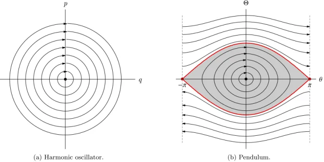
2.1.6 Basic examples of Hamiltonian systems . . . 24

2.2 Planetary systems in Hamiltonian mechanics . . . 29

2.2.1 The two-body problem . . . 29

2.2.2 The planetary problem . . . 34

2.3 Elements of Hamiltonian perturbation theory . . . 38

2.3.1 First order perturbation theory . . . 38

2.3.2 An introduction to adiabatic theory . . . 40

2.3.3 Application of the adiabatic theory to resonant capture . . . 42

3 Two planets – The structure of resonant pairs and capture into mean motion resonance 45 3.1 Structure of first-order mean motion resonances . . . 45

3.1.1 First and higher order expansions of the Hamiltonian in the eccentricities . . . 47

3.1.2 Equilibrium points of the averaged Hamiltonian . . . 47

3.1.3 Frequencies in the limit of small amplitude of libration . . . 49

3.2 Capture into resonance by type-I migration . . . 52

3.2.1 Convergent inward migration in disc and resonant capture . . . 53

3.2.2 Planet-disc interactions and evolution in mean motion resonance . . . 56

4 Three-planet systems and the near-resonant population 63 4.1 The near-resonant population . . . 63

4.1.1 Methods and physical setup . . . 64

4.2 Analytical model for three resonant planets . . . 66

4.2.1 Resonant equilibrium points . . . 68

4.2.2 Resonant repulsion for three-planets systems . . . 69

4.3 A scenario for dissipative evolution of three-planet systems . . . 70

4.3.2 Analytical maps . . . 71

4.3.3 Numerical simulations . . . 73

4.4 Results . . . 77

4.4.1 Probabilistic measure of a resonant configuration in Kepler-305, YZ Cet and Kepler-31 . . . . 77

4.4.2 The 5:4 – 4:3 resonant chain on Kepler-60 and other near-resonant systems with k > 3 . . . . 78

4.5 Conclusions . . . 78

5 The onset of instability in resonant chains 81 5.1 Introduction . . . 81

5.2 2 Planets . . . 82

5.3 3 Planets . . . 88

5.3.1 Numerical stability maps for N = 3 and k = 3 . . . 88

5.3.2 Numerical and analytical investigation of the phenomenon . . . 89

5.3.3 Rescaled Hamiltonian and new set of canonical variables . . . 90

5.3.4 Purely resonant dynamics . . . 93

5.3.5 The synodic contribution . . . 95

5.3.6 Dependence on k . . . 106

5.4 N Planets . . . 108

6 Extreme secular excitation of eccentricity inside mean motion resonance 111 6.1 Small bodies driven into star-grazing orbits by planetary perturbations . . . 112

6.2 Planetary Hamiltonian . . . 113

6.3 Studying the averaged Hamiltonian . . . 115

6.4 Effect of short-range forces . . . 118

6.5 Results . . . 119

6.6 Conclusions . . . 124

7 Conclusions 127 7.1 Future perspectives . . . 129 A Integrable approximation for two-planet mean motion resonant dynamics 141 B Reduced Hamiltonian to a common planetary mass factor for three resonant planets 145

C Some useful Mathematica code snippets for perturbation theory 147

D Mathematica code used in Chapter 6 149

Chapter 1

Introduction

1.1

A brief history of Planetary Science

The study of dynamics was triggered by the need to understand the movement of the planets in our Solar System, our astronomical home. There have been a few major milestones in our understanding of their motion. The first was heliocentric theory, put forth as early as the 3rd century BC by Aristarchus of Samos but gaining scientific and historical significance in the 16th century with Nicolaus Copernicus, who showed that orbits centred at the Sun provide a much simpler description of the motion of the planets. The second innovation was the introduction of Kepler’s laws of planetary motion by Johannes Kepler between 1609 and 1619. They are three empirical laws that describe the motion of the planets around the Sun on elliptical orbits, an approximation valid at least on short timescales. The third innovation was given by Newtonian theory, derived by Isaac Newton and first published in 1687 in his Philosophiæ Naturalis Principia Matematica. Newton’s laws of motion, his law of universal gravitation and the techniques of differential and integral calculus allowed him to derive Kepler’s laws, even introducing some corrections and developments, like the fact that parabolic and hyperbolic motion are also allowed. Newton also realised that the planets’ mutual interactions may be responsible for significantly modifying their orbits over time. Theoretical applications of Newtonian theory have been very successful and enlightening, such as the Lagrange-Laplace theory on the secular evolution of the planets’ orbits in the 1770’s. Moreover, they drove the development of perturbation theory, and yielded theoretical results such as Poincar´e’s proof around 1900 of the non-integrability of the three-body problem and the coexistence of order and chaos even in seemingly ordered systems, which completely changed our understanding of dynamical systems. One last improvement in the understanding of gravitational interactions was Einstein’s 1916 theory of general relativity, which gives a geometrical description of the origin of the gravitational force (a question which Newton admitted he could not address) and an explanation for a few quirks of the dynamics of the planets, most notably the precession of Mercury. Nonetheless, classical Newtonian dynamics is very accurate and adequate to describe the motion of the planets and small bodies of the Solar System. It should suffice to say that Newtonian theory was not only able to prove Kepler’s empirical laws in describing why the planets move as they do, but it even allowed to predict with astonishing accuracy the position of unseen planets, as in the case for Neptune, discovered by Le Verrier “with the point of his pen” (as F. Arago put it) and observed by J. G. Galle and H. L. d’Arrest in Berlin in 1846 following Le Verrier’s calculations.

It is worth recalling our classification of the orbiting bodies of the Solar System, with the definitions given in 2006 by the International Astronomical Union. A planet is a celestial body that orbits around the Sun, has a large enough mass that it has an approximatively spherical shape due to its own gravity, and dominates the local dynamics around its orbit. There are 8 planets known in our Solar System, some of which having natural satellites (moons) around them: they are Mercury, Venus, Earth, Mars, Jupiter, Saturn, Uranus and Neptune in order of their distance to the Sun, usually measured in terms of the semi-major axis of their Keplerian ellipse. Additionally, there are the dwarf planets (like Pluto, Eris, Ceres, Makemake, Haumea, some of which having moons of their own) and a vast number of additional small Solar System bodies, such as the comets, the asteroids, the trojans and the trans-Neptunian objects. In a way, the task of Celestial Mechanicians is to verify that Newtonian theory can explain all the aspects of the dynamics of these orbiting bodies that we observe and to understand the dynamical features of the Solar System. And indeed, this task is still not complete, as many details of the dynamics exhibited by our Solar System need to be investigated and explained, such as the orbital distribution of the distant Kuiper belt objects, which has been proposed as evidence for an additional, yet unseen ninth planet orbiting our Sun. However, in the last 20 years the attention of many astronomers has turned far, far away from our Solar System.

●_● ● ● ● ● ● ● ● ● ● ● ● ● ● ● ● ● ● ● ● ● ● ● ● ● ● ● ● ● ● ● ● ● ● ● ● ● ● ● ● ● ● ● ● ● ● ● ● ● ● ● ● ● ● ● ● ● ● ● ● ● ● ● ● ● ● ● ● ● ● ● ● ● ● ● ● ● ● ● ● ● ● ● ● ● ● ● ● ● ● ● ● ● ● ● ● ● ● ● ● ● ● ● ● ● ● ● ● ● ● ● ● ● ● ● ● ● ● ● ● ● ● ● ● ● ● ● ● ● ● ● ● ● ● ● ● ● _●● ● ● ● ● ● ● ● ● ● ● ● ● ● ● ● ● ● ● ● ● ● ● ● ● ● ● ● ● ● ● ● ● ● ● ● ● ● ● ● ● ● ● ● ● ● ● ● ● ● ● ● ● ● ● ● ● ● ● ● ● ● ● ● ● ● ● ● _● ● ● ● ● ● ● ● ● ● ● ● ● ● ● ● ● ● ● ● ● ● ● ● ● ● ● ● ● ● ● ● ● ● ● ● ● ● ● ● _● ● ● ● ● ● ● ● ● ● ● ● ● ● ● ● ● ● ● ● ● ● ● ● ● ● ● ● ● ● ● ● ● ● ● ● ● ● ● ● ● ● ● ● ● ● ● ● ● ● ● ● ● ● ● ● ● ● ● ● ● ● ● ● ● ● ● ● ● ● ● ● ● _● ● ● ● ● ● ● ● ● ● ● ● ● ● ● ● ● ● ● ● _● ● ● ● ● ● ● ●_● ● ● ● ● ● ● ● ● ● ● ● ● ● ● ● ● ● ● ● ● ● ● ● ● ●● ● ●● ● ● ● ● ● ● ● ●●● ● ● ● ● ● ● ● ● ● ● ● ● ● ● ● ● ● ● ● ● ● ● ● ● ● ● ● ● ● ● ● ● ● ● ● ● ● ● ● ● ● _● ● ● ● ● ● ● ● ● ● ● ● ● ● ● ● ● ● ● ●● ● ● ● _● ● ● ● ● ● ● ● ● ● ● ● ● ● ● ● ● ● ● ● ● ● ● ● ● ● ● ● ● ● ● ● ● ● ● ● ● ● ● ● ● ● ● ● ● ● ● ● ● ● ● ● ● ● ● ● ● ● ● ● ● ● ● ● ● ● ● ● ● ● ● ● ● ● ● ● ● ●_● ● ● ● ● ● ● ● ●● ● ● ● ● ● ● ● ● ● ● ● ● ● ● ● ● ● ● ● ● ● ● ● ● ● ● ● ● ● ● ● ● ● ● ● ● ● ● ● ● ● ● _● ● ● ● ● ● ● ● ● ● ● ● ● ● ● ● ● ● ● ● ● ● ● ● ● ● ● ● ● ● ● ● ● ● ● ● ● ● ● ● ● ● ● ● ● ● ● ● ● ● ● ● ● ● ● ● ● ● ● ● ● ● ● ● ● ● ● ● ● ● ● ● ● ● ● ● ● ● _● ● ● ● ● ● ●● ● ● ● ● ● ● ● ● ● ● ● ● ● ● ● ● ●● ● ● ●● ● ● ● ● ● ● ● ● ● ● ● ● ● ● ● ● ● ● ● ● ● ● ● ● ● ● ● ● ● ■ ■ ■■ ■ ■ ■ ■ ■ ■ ■ ■ ■ ■ ■ ■ ■ ■ ■ ■ ■ _■ ■ ■ ■ ■ ■ ■ ■ ■ ■ ■ ■ ■ ■ ■ ■ ■ ■ ■ ■ ■ ■ ■ ■■ ■ ■ ■ ■■ ■ ■ ■ ■ ■ ■ ■ ■ ■_■ ■■ ■ ■ ■ ■ ■ ■ ■■ ■ ■ ■ ■ ■ ■ ■ ■ ■ ■ ■■■■ ■ ■ ■ ■ ■ ■ ■ ■ ■ ■ ■ ■ ■ ■ ■ ■ ■ ■■ ■ ■ ■ ■ ■_■ ■ ■ ■ ■ ■ ■ ■ ■ ■ ■ ■ ■ ■ ■ ■ ■ ■ ■ ■ ■ ■ ■ ■ ■ ■ ■ ■ ■ ■ ■ ■ ■ ■ ■ ■■ ■ ■ ■ ■ ■ ■ ■ ■ ■ ■ ■ ■ ■ ■ ■ ■ ■ ■■ ■ ■ ■ ■ ■ ■ ■ ■ ■ ■ ■ ■ ■ ■ ■ ■ ■ ■ ■ ■ ■ ■ ■ ■■ ■ ■ ■ ■ ■ ■ ■■ _■ ■ ■ ■ ■ ■ ■ ■ ■ ■ ■ ■ ■ ■ ■ ■ ■ ■ ■ ■ ■ ■ ■ ■ ■ ■ ■ ■ ■ ■ ■ ■ ■ ■ ■ ■ ■ ■ ■ ■ ■ ■ ■ ■ ■ ■ ■■ ■ ■ _■ ■ ■ _■ ■ ■ ■ ■ ■ ■ ■ ■ ■ ■ ■ ■ ■ ■ ■ ■ ■ ■ ■ ■ ■ ■ ■ ■ ■ ■■ ■ ■ ■ ■ ■ ■ ■ ■■ ■ ■ ■ ■ ■ ■ ■ ■ ■ ■ ■ ■ ■ ■ ■ ■ ■ ■ ■ ■ ■ ■ ■ _■■ ■ ■ ■ ■ ■ ■ ■ ■ ■ ■ ■ ■ ■ ■ ■ ■ ■ ■ ■■ ■■ ■ ■ ■■ ■ ■ ■ ■ ■ ■ ■ ■ ■ ■ ■ ■ _■ ■ ■ ■ ■ ■ ■■ ■ ■ _■ ■ ■ ■ ■ ■ ■ ■ ■ ■ ■ ■ ■ ■ ■ ■ ■ ■■ ■ ■ ■ ■ ■ ■ ■ ■ ■ ■ ■ ■ ■ ■ ■ ■■ ■ ■ _■ ■ ■ ■ ■ ■■ ■ ■ ■ ■ ■ ■ ■ _■ ■ ■ ■ ■■ ■ ■ ■ ■ ■ ■ ■ ■ ■ ■ ■ ■ ■ ■ ■ ■ ◆ ◆ ◆ ◆ ◆ ◆ ◆ ◆ ◆ ◆ ◆◆ ◆ ◆ ◆ _◆ ◆ ◆ ◆ ◆ ◆ ◆◆ ◆ ◆ ◆ ◆ ◆ ◆ ◆ ◆ ◆ ◆ _◆ ◆ ◆ ◆ ◆ ▲ ▲ ▲ ▲ ▲ ▲ ▲ ▲ ▲ ▲ ▲ ▲ ▲ ▲ ▲ ▲ ▲ ▲ ▲ ▲ ▲ ▲ ▲ _▲ ▲ ▲ ▲ ▲ ▲ ▲ ▲ ▲ ▲ ▲ ▲ ▲ ▲ ▲ ▲ ▲ ▲ ▲ ▲ ▲ ▲ ▲ ▲ ▲ ▲ ▲ ▲ ▲ ▲ ▲ ▲ ▲ ▲ ▲▲ ▲ ▲ ▲ ▲ ▲▲ ▲ ▲ ▲ ▲ ▲ ▲ ▲ ▲ ▲ ▲ ▼ ▼ ○ ○○ ○ ○ ○ □ □ □ □ □ □ □□ □ ◇ ◇ ◇ ◇ △△ △ Neptune Mercury Venus Earth Mars Jupiter Saturn Uranus 0.01 0.10 1 10 100 1000 a (AU) 0.10 1 10 100 1000 104 Mass (MEarth) ● RV ■ Transit ◆ Imaging ▲ Microlensing ▼ Pulsation Timing Variations ○ Pulsar Timing □ Eclipse Timing Variations ◇ Transit Timing Variations △ Orbital Brightness Modulation

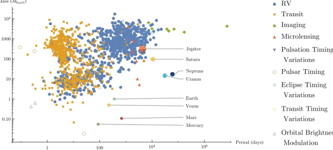
Figure 1.1: Semi-major axes a and masses of detected exoplanets (the coloured markers). The semi-major axis is measured in Astronomical Units (AU), with 1 AU being the semi-major axis of Earth’s orbit. The colours and markers indicate the different detection methods (see legend on the right), most planets having been detected by the Radial Velocity (RV) or Transit method (see main text). The Solar System planets are also shown for comparison. Data was obtained from the Nasa Exoplanet Archive https://exoplanetarchive.ipac.caltech.edu/.

1.1.1

The discovery of exoplanetary systems

Until very recently, the Solar System was the only known planetary system, and as far as we could tell even the only existent one. This unlikely possibility was ruled out by observations in 1995, with the detection of a doppler-shift signal in the movement of the star 51 Pegasi (a method called Radial Velocity, see below), the first evidence of an exoplanet orbiting a main sequence G-type star and thus modifying its motion in a detectable way1

[Mayor and Queloz(1995)]. The planet 51 Peg b has a mass at least half that of Jupiter and an orbital period of only about 4.2 days. As such, it is the prototype of the now called hot Jupiters which, as the name suggests, are Jupiter-like planets which orbit very close to their host star. The possibility that a planet similar to Jupiter could have such a narrow orbit came as a shock to astronomers, who thought that other planetary systems, if they existed, would be more or less like ours. Soon enough, it was realised that the Solar System is not the typical planetary system. For example, observations now indicate that more than 50% of stars have planets that do not have analogues in the Solar System [Morbidelli(2018)], while only_{∼ 1% of observed systems have a gas giant planet} relatively far away and on a low eccentricity orbit like Jupiter [Winn and Fabrycky(2015)].

These statements have been made possible by more then two decades of observations of exoplanetary systems. The number of planets discovered every year has been growing exponentially, with a doubling time of about 2 years. As of 21 June 2019 there are 4003 confirmed exoplanets, with 1704 planets found in 678 multi-planetary systems. This represents a massive sample, telling us that planets can be much more diverse than we could ever imagine, and opening completely new physical and dynamical questions, all the while giving us many more clues in the process of planetary formation and evolution. There are of course many interesting aspects that emerge from the study of the current exoplanet population, but in the interest of brevity we review below those which are most significant in the context of this thesis.

1.1.2

The exoplanets sample

Figures 1.1 and 1.2 show the detected exoplanets up until 21 June 2019, in terms of planetary mass versus semi-major axis of their orbit or orbital period. Each marker is a detected planet, and the Solar System planets are included for comparison. From these figures, especially Figure 1.2, one can make out the different classes of exoplanets. The so called hot Jupiters (such as the already mentioned 51 Peg b) are massive planets, with masses

1_{The discovery was made on 6 October 1995 by M. Mayor and D. Queloz using observations gathered at the Observatoire de}

● ● ● ● ● ● ● ● ● ● ● ● ● ● ● ● ● ● ● ● ● ● ● ● ● ● ● ● ● ● ● ● ● ● ● ● ● ● ● ● ● ● ● ● ● ● ● ● ● ● ● ● ● ● ● ● ● ● ● ● ● ● ● ● ● ● ● ● ● ● ● ● ● ● ● ●● _● ● ● ● ● ● ● ● ● ● ● ● ● ● ● ● ● ● ● ● ● ● ● ● ● ● ● ● ● ● ● ● ● ● ● ●● ● ● ● ● ● ● ● ● ● ● ● ● ● ● ● ● ● ● ● ● ● ● ● ● ● ● ● ● ● _●● ● ● ● ● ● ● ● ● ● ● ● ● ● ● ● ● ● ● ● ● ● ● ● ● ● ● ● ● ● ●● ● ● ● ● ● ● ● ● ● ● ● ● ● ● ● ● ● ● ● ● ● ● ● ● ● ● ● ● ● ● ● ● ● ● ● ● ● ● _● ● ● ● ● ● ● ●● ● ● ● ● ● ● ● ● ● ● ● ● ● ● ● ● _● ● ● ● ●● ● ● ● ● ● ● ● ● ● ● _● ● ● ● ● ● ● ● ● ● ● ● _● ● ● ● ● ● ● ● ● ● ● ● ● ● ● ● ● ● ● ● ● ● ● ● ● ● ● ● ● ● ● ● ● ● ● ● ● ● ● ● ● ● _● ● ● ● ● ● ● ● ● ● ● ● ● ● ● ● ● ● ● ● ● ● _● ● ● ● ● _● ● ● ● ● ● ● ● ● ● ● ● ● ● ● ● _● ● ● ● ● ● ● ●● ● ● ● ● ● ● ● ● ● ● ● ● ● ● ● ● ● ● ● ● ● ● ● ● ● ● ● ● ● ● ● ● ● ● ● ● ● ●●● ● ● ● ● ● ● ● ● ● ● ● ● ● ● ● ● ● ● ● ● ● ● ● ● ● ●● ● ● ● ● ● ● ● ● ● ● ● ● ● ● _● ● ● ● ● ● ● ● ● ● ● ● ● ● ● ● ● ● ● ● ● ● ● ● ● _● ● ● ● ● ● ● ● ● ● ● ● ● ● ● ● ● ● ● ● ● ● ● ● ● ● ● ● ● ● ● ● ● ● ● ● ● ● ● ● ● ● ● ● ● ● ● ● ● ● ● ● ● ● ● ● ● ● ● ● ● ● ● ● ● ● ● ● ● ● ● ● ● ● ● ● ● ● ● ● ●● ● ● ● ● ● ● ● ● ● ● ● ● ● ● ● ● ● ● ● ● ● ● ● ● ● ● ● ● ● ● ● ● ● ● ● ● ● ● ● ● ● ● ● ● ● ● ● ● ● ● ● ● _● ● ● ● ● ● ● ● ● ● ● ● ● ● ● ● ● ● ● ● ● ● ● ● ● ● ● ● ● ● ● ● ● ● ● ● ● ● ● ● ● ● ● ● ●● _● ● ● ● ● ● ● ● ● ● ● ● ● ● ● ● ● ● ● ● ● ● ● ● ● ● ● ● ● ● ● ● ● ● ● ● ● ●● _● ● ● ● ● ● ● ● ● ● ● ● ●● ● ● ● ● ● ● ● ● ● ● ● ● ● ● ● ● ● ● ● ● ● ●● ● ● ● ● ● ● ● ● ● ● ● ● ● ● ● ● ● ● ● ● ● ● ● ● ● ● ● ● ● ● ● ● ■ ■ ■ ■ ■■ ■ ■ ■ ■ ■ ■ ■ ■ ■ ■ ■ ■ ■ ■ ■ ■ ■ ■ ■ ■ ■ ■ ■ ■ ■ ■ ■ ■ ■ ■ ■ ■ ■ ■ ■ ■ ■ ■ ■ ■ ■ ■ ■ ■ ■ ■ ■ ■ ■■ ■ ■■ ■ ■ ■ ■ ■ ■ ■ ■ ■ _■ ■ ■ ■ ■ ■ ■ ■ ■ ■ ■ ■ ■■ ■ ■ ■ ■ ■ ■ ■ ■ ■■ ■ ■ ■ ■ ■ ■ ■ ■ ■■ ■ ■ ■ ■ ■ ■ ■ ■ ■ ■ ■■ ■■ ■ ■ ■ ■ ■ ■■ ■ ■ ■ ■ ■ ■ ■ ■ ■ ■ ■■ ■ ■ ■ ■ ■ ■ ■ ■ ■ _■ ■ ■ ■ ■ ■ ■ ■ ■ ■ ■ ■ ■ ■ ■ ■ ■ ■ ■ ■ ■ ■ ■ ■ ■ ■ ■ ■ ■ ■ ■ _■ ■ ■ ■ ■ ■ ■ ■■ ■ ■ ■ ■■ ■ ■ ■ ■ ■ ■■ ■ ■ ■ ■ ■ ■ ■ ■ ■ ■ ■ ■ ■ ■ ■ ■ ■ ■ ■ ■■ ■ ■ ■ ■ ■ ■ ■ ■ ■ ■ ■ ■ ■ ■ ■ ■ ■ ■ ■ ■ ■ ■ ■ ■ ■ ■ ■ ■ ■ ■ ■ ■ ■ ■ ■■ ■ ■ ■ ■ ■■ ■ ■ ■ ■ ■ _■ ■■ ■ ■ ■ ■ ■ ■ ■ ■ ■ ■ ■ ■ ■ ■ ■ ■ ■ ■ ■ ■ ■ ■ ■ ■ ■ ■ ■ ■ ■ ■ ■ ■ ■ ■■■ ■ ■ ■ ■ ■ ■ ■ ■ ■ ■ ■ ■ ■ ■ ■ ■■_■ ■ ■ ■ ■ ■ ■ ■ ■■ ■ ■ ■ ■ ■■ ■ ■ ■ ■ ■ ■ ■ ■ ■ ■ ■ ■■ ■ ■ ■ ■ ■ ■ ■ ■ ■ ■ ■ ■ ■ ■ ■ ■ ■ ■ ■ ■ ■■ ■ ■ _■ ■ ■ _■ ■ ■ ■ ■ ■ ■ ■ ■ ■ ■ ■ ■ ■ ■ ■ ■ ■ ■ ■ ■ ■ ■ ■ ■ _■ ■ ■ ■ ■_■ ■ ■ ■ ■ ■■■■ ■ ■■■ ■ ■ ■ ■ ■ ■ ■ ■ ■■ ■ ■ ■ ■ ■ ■ ■ ■ ■ ■ ■ ■ ■ ■ ■ ■ ■ ■ ■ ■ ■ ■_■ ■ ■ ■ ■ ■ ■ ■ ■ ■ ■ ■ ■ ■ ■ ■ ■ ■ ■■ _■■ ■ ■ ■ ■ ■ ■ ■ ■ ■ ■ ■ ■ ■ ■ ■ ■ ■ ■ ■■ ■■ ■ ■ ■ ■ ■ ■ ■ ■ ■ ■ ■ ■ ■ ■■ ■ ■ ■ ■ ■ ■ ■ ■ ■ ■ _■ ■ ■ ■ ■ ■ ■ ■■ ■ ■ _■ ■ ■ ■ ■ ■ ■ ■ ■ ■ ■ ■ ■ ■ ■ ■ ■ ■ ■ ■ ■■ ■ ■ ■ ■ ■ ■ ■ ■ ■ ■ ■ ■ ■ ■ ■ ■ ■ ■ ■ ■ ■ ■■ ■ ■ ■ ■ ■ ■ ■ ■ _■ ■ ■ ■ ■ ■ ■ ■■ ■ ■ ■ ■ ■ ■ ■■ ■ ■ ■ ■■_■ ■ ■ ■ ■■ ■ ■ ■ ■ ■ ■ ■ ■ ■ ■ ■ ■ ■ ■ ■■ ■ ■ ■ ■ ■ ■ ■ ■ ■ ■ ■ ■ ■ ■ ■ ■ ■ ■ ■ ■ ■ ■ ■ ■ ■ _■ ■ ■ ■ ■ ■ ■ ◆ ◆ ◆ ◆ ◆_◆ ◆ ▲ ▲ ▲ ▲ ▲ ▲ ▲ ▼ ▼ ○ ○○ ○ ○ □ □ □ □ □ □ □□ □ □ ◇ ◇ ◇ ◇ ◇ ◇ ◇ ◇ ◇ ◇ ◇ ◇ △△ △ Neptune Mercury Venus Earth Mars Jupiter Saturn Uranus 1 100 104 ₁₀6 Period (days) 0.10 1 10 100 1000 104 Mass (MEarth) ● RV ■ Transit ◆ Imaging ▲ Microlensing ▼ Pulsation Timing Variations ○ Pulsar Timing □ Eclipse Timing Variations ◇ Transit Timing Variations △ Orbital Brightness Modulation

Figure 1.2: Same as Figure 1.1, but with the orbital period measured in (Earth’s) days on the horizontal axis.

ranging from 102_M

⊕ to a few 104M⊕ (1M⊕ = 1 Earth mass), with a very short orbital period between 1 and

100 days, which are thought to be physically similar to our gas giants Jupiter and Saturn, and occupy the top left corner in both plots. Although they were the first planets to be detected (as they are the easiest ones, being so massive and with a short orbital period), more recent data suggests that only less than a few percent of stars host a hot Jupiter [Howard et al.(2012), Wright et al.(2012), Winn and Fabrycky(2015)]. The top right corner is populated by the cold or normal Jupiters, and we see that our Jupiter actually falls within the boundaries of this group. The planets in the bottom left corners have masses between about 1 to a few tens of Earth’s masses and a period of less than about 100 days, and are called Super-Earths or Mini-Neptunes, depending on their composition (see Section 1.3). These planets are thought to orbit up to 50% of Sun-like stars ([Mayor et al.(2011)]; [Howard et al.(2012)]; [Fressin et al.(2013)]; [Petigura et al.(2013)]), therefore posing an enormous constraint on planet formation and evolution models, and their dynamics will be the main subjects of this thesis. The rest of the parameter space (where all of the Solar System’s planets except Jupiter are located) is left empty, but mostly because of our limitations in detecting these planets.

The different colours/markers in Figures 1.1 and 1.2 represent the detection methods used to discover the planets. So far, the two main detection methods are the Radial Velocity (RV) and the Transit photometry methods. The RV method (also called Doppler spectroscopy) exploits the fact that the gravitational pull of a massive enough body orbiting a star will force said star to orbit around the system’s centre of mass, and cause a detectable periodic Doppler shift of the star’s spectrum. With the transit method, one essentially observes eclipsing planets which cause a small, regular decrease in the brightness of the star. The two surveys from NASA’s Kepler and K2 missions have been extremely successful in finding thousands of planets in only a few years, and missions such as TESS and PLATO will expand on this legacy. Other detection methods include direct imaging, microlensing, and astrometry (thanks to the Gaia mission), and are expected to yield in the future a large amount of new data which will allow us to fill the current observational gaps still present in Figures 1.1 and 1.2, and to better describe the nature of exoplanetary systems.

1.1.3

The Solar System in perspective and implications of the exoplanets sample

Observing thousands of planetary systems has many consequences. On the one hand it puts our own into context, and on the other it actually allows us to better understand the processes that shaped the Solar System. For example, we did not expect that planets like hot Jupiters could exist, and since the possibility that they formed where they are now may seem unlikely, processes like orbital transport within the protoplanetary disc become now conceivable (e.g. [Lin et al.(1996), Kley and Nelson(2012), Beaug´e and Nesvorn´y(2012)]; however, see also e.g. [Batygin et al.(2016), Bailey and Batygin(2018)]). As we shall see, this so-called planetary migration is indeed thought to play a major role in shaping the orbits of planets such as Super-Earths and Mini-Neptunes. This and many other realisations come from the study of the physical processes acting on distant planetary systems, and

leak into the understanding of the formation and evolution of our own.

It is important to realise that different exoplanet detection methods allow to obtain different physical and orbital parameters, and are more or less sensitive to different regions of parameter space, which is why the two plots in Figures 1.1 and 1.2 show some differences. For example, RV detections usually yield the planetary mass mpl only

via mplsin I (where I is the angle between the normal to the orbital plane and the line-of-sight of the observer2),

the orbital period, the eccentricity and the direction of the periastron (the point along the orbit that is closest to the star) of the planet’s orbit from the signal’s amplitude, periodicity, shape and phase respectively. Instead, transit detections allow to get the orbital period from the periodicity of the signal and the radius of the planet from the shape of the signal. More precisely, these two methods give the planetary mass and radius with respect to that of the star. Moreover, if an additional unseen planet is disturbing the transiting one, small Transit Time Variations (TTV) in the signal of the observed planet can allow the indirect discovery of the undetected one. In some cases one can observe the same system with multiple methods. Or, if one is not interested in specific systems but on the general distribution of the physical and orbital parameters of exoplanets, statistical methods can be used (e.g. assuming a uniform distribution of cos I to extract the distribution of planetary masses from RV detections, or breaking the mass-eccentricity degeneracy in the TTV signals [Wu and Lithwick(2013)]). In any case, making a complete exoplanet demographics study is very hard and one needs to be extremely careful before drawing absolute conclusions. Moreover, planetary systems like our own are not yet detectable, since all planets but Jupiter are either too small or have too large orbital periods to be observed.

However, it remains clear from Figures 1.1 and 1.2 that any model of planetary formation must be able to explain the formation of planets very different from those of our Solar System. Then, the observed architecture of planetary systems challenges the Celestial Mechanician to explain how these orbital configurations can emerge. I therefore recall in the next section the main points in our current understanding of planetary formation and early evolution, while I give in Section 1.3 the motivation for the dynamical investigations that are described in this thesis.

1.2

Planetary formation

Planetary formation is a byproduct of star formation. Molecular clouds that are massive enough collapse gravi-tationally to form protostars in so-called star forming regions. While a protostar is forming, by conservation of angular momentum some material does not fall into the protostar but forms a relatively flat, rotationally supported disc around it. In the mostly credited core-accretion scenario [Pollack et al.(1996)], planets are then thought to form from the material contained in such a disc: the rocky planets or the cores of the gas giants are accreted from the rocky components while giant planets’ atmospheres represent gaseous material that has been accreted by sufficiently massive cores formed within the lifetime of the disc. For this reason, the discs observed routinely around young stars are called protoplanetary discs. Very recently, in [Keppler et al.(2018)], the first evidence of a forming planet with a mass around 2 – 20 Jupiter masses observed still embedded in and interacting with its_{∼ 5} Mys old disc was announced (see also [M¨uller et al.(2018)]).

The growth from the micron-sized dust particles detected in these young discs to fully formed planets is usually divided into steps corresponding to different physical processes: from dust to small pebbles, to planetesimals, to planetary embryos, to planetary cores, to planets in all their shapes and forms. We give a quick review of these accretion processes in Subsect. 1.2.2. However, before we delve into the question of the formation of the actual planets, it is important to realise that the protoplanetary discs set the stage for planet formation, which is why it is crucial to understand the physical properties and mechanisms that control their structure and evolution. This is still a topic of vast research, and a full discussion is beyond the scope of this text. We shall recall below the most important concepts that are needed in the context of this thesis.

1.2.1

Protoplanetary discs

The idea of a flat disc of material orbiting our Sun from which the planets formed dates back to the eighteenth century with thinkers such as Kant and Laplace. Nowadays, discs of gas and dust are detected regularly around young stars, either because of the infrared excess in the observed spectral energy distribution coming from the forming star, or by direct imaging with instruments such as ALMA, SPHERE and GPI. Measuring the disc frequency against stellar age yields a lifetime of protoplanetary discs of around 3 – 10 My [Hern´andez et al.(2007)].

2_{This is because we only measure the movement of the star that happens along our line-of-sight, so we cannot tell apart a small}

planet whose apparent motion takes place along the line-of-sight (I ' 90◦), or a massive planet whose orbit appears to be almost face-on (I ' 0◦).

Figure 1.3: Diagram of a protoplanetary disc (adapted with permission from [Lesur(2018)]).

The typical structure of protoplanetary discs is shown in Figure 1.3. Their bulk composition is mostly gas (mainly H/He), with only∼ 1% of their mass being made of dust (micron-sized grains). The gas feels a pressure in addition to the star’s gravity, and so gas molecules rotate around the star with an orbital velocity that can be slightly different from the Keplerian velocity vK = pGM∗/r (where G is the gravitational constant, M∗ is the mass of

the central star and r is the radial distance from the star), and this influences the motion of small solid particles dynamics by aerodynamic coupling, as we shall see. Moreover, locally there can be enhancements in the solid-gas ratio which allow for different accretion processes to take place. Ultimately, the 1% dust is what makes the telluric planets and the gas giants’ cores, so the study of how the dust particles can clump together and interact with the surrounding gas is of great interest. In the description of the equilibrium structure of protoplanetary discs, two simplifications are helpful [Armitage(2010)]. The first is the assumption that the disc’s mass is negligible compared to that of the star, so self-gravity can be neglected (however this may not always be the case, especially early in the formation of the protostar). The second is that the vertical thickness of the disc H(r) is small (of the order of a few percent, see below) compared to the orbital radius r (this is true in conditions of relativeley low temperatures, as we see below).

Concerning the radial structure of the disc, probably the most important parameter is the vertically averaged surface density Σ =R ρ dz, where ρ is the density and z is the direction normal to the disc. In truth, one cannot always avoid the presence of azimuthal structures such as vortices (which might play a role in planetesimal formation, see next subsection), spiral waves (important in the treatment of planet-disc interactions and migration, see Subsect. 1.2.3), eccentric cavities due to binary companions to the main star, etc. However, to first approximation in an undisturbed, (nearly) radially symmetric disc rotating in equilibrium around a single star, one considers Σ = Σ(r) as function of r alone. In the most simple case one imagines a power law profile Σ(r) = Σ0(r/r0)−αΣ, for some

constant αΣ> 0 and some reference orbital separation r0. In the case of the Solar System, one approach to obtain

such a density profile has been to divide up the space around the Sun in rings centred at the location of the planets, and use the amount of material now present in these rings rescaled to solar abundances to give a lower bound to the original surface density. This yields the so-called Minimum-Mass Solar Nebula (MMSN) prescription Σ(r)' 1.7×103_{g cm}−2_{(r/1 AU)}−3/2_{(e.g. [Hayashi(1981)]); integrating over a reasonable extension of the disc one}

would get a total disc mass of_{' 0.01M}, consistent with the assumption that the gravity of the Sun is dominant. However, we now know there’s no reason that the initial material should not move radially during the disc’s lifetime

F

z gz

g

Figure 1.4: Vertical structure of a thin protoplanetary disc. A parcel of gas (in grey) at a radial distance r and a height z feels a vertical gravitational force gz∼ (GM∗/r3)z for z  r. This is balanced by the pressure gradient

under vertical hydrostatic equilibrium.

so different power law profiles cannot be excluded. Note moreover that a power law is always an approximation for Σ(r), and we now have observational evidence that rings and gaps do form routinely in protoplanetary discs thanks to ALMA (e.g. [Dullemond et al.(2018)]).

Concerning the vertical structure of the disc, consider a gas parcel at radial distance r and height z from the disc mid-plane (Figure 1.4). The vertical component of the gravitational force is gz = ((GM∗)/(r2+ z2))(z/√r2+ z2)∼

(_GM∗/r3)z for z r. Assuming that the gas is in vertical hydrostatic equilibrium so that the gravitational force

due to the star is balanced by pressure, we get (_GM∗/r3)z = −(1/ρ) dP/ dz where ρ is the density and P the

pressure. Assuming a perfect gas law P µ = RρT as an equation of state for the pressure, µ being the mean molecular mass, R the ideal gas constant and T the temperature, we solve the force-balance equation and get a vertical density profile ρ(z) = ρ0exp(−z2/(2H2)) with H(r) = (R/(µT r3))1/2, called the vertical scale-height of

the disc, which depends on the disc’s physical parameters. Notice that now one can write ρ0= 1/√2π(Σ/H). If

the disc is vertically isothermal the equation for the pressure can be written as P = ρc2

s, where cs is the sound

speed, so the scale-height becomes H = cs/ΩK, where ΩK =pGM∗/r3 is the Keplerian orbital frequency at the

radial distance r. One also defines h = H/r = cs/vK called the aspect ratio of the disc. This parameter gives

the vertical geometrical thickness of the disc, and depends on the temperature T (r). The temperature profile is usually sculpted by viscous heating at small distances from the central star and by stellar irradiation at larger distances. Assuming a power law for T one gets h(r) = H/r = zscale(r/r0)βf. The exponent βf is usually positive

for T distributions shallower than 1/r, as those resulting from viscous and irradiation heating; it is called flaring index. Calculations of the equilibrium temperature of the disc lead to values of h(r) of the order of a few to several percents, in agreement with observations of discs, and validating the approximation h_1.

Other physical parameters of the disc (such as the viscosity, turbulence, ionisation fraction, opacity), and the effect of magnetic phenomena are also important. This is the subject of a vast research, and I refer to [Turner et al.(2014), Armitage(2015), Lesur(2018)] for an extensive treatment of these processes. With the ba-sic understanding of disc structures outlined above, we can now turn to the problem of planetary formation in protoplanetary discs.

1.2.2

Building the planets: Overview of accretion processes

To go from microscopic dust to planets we need to grow_{∼ 13 orders of magnitude in size, or ∼ 40 orders of} magni-tude in mass. The details of the accretion processes at play are usually split up in stages according to the different scales at which they occur. In general, these processes have to be efficient and fast [Morbidelli(2018)], and models of planetary formation must explain the presence of planets in all their shapes and forms (terrestrial, gas giants, ice giants, Super-Earths, Mini-Neptunes, ...): this is clearly a difficult problem. For this thesis, we will not need to go too much into the details, and we will concentrate mainly on the formation up to Super-Earths/Mini-Neptunes. We start with the micron-sized dust particles which are observed in discs around young stars, and may originate from interstellar medium and/or condense in the disc itself. The aerodynamic coupling between solid particles and gas is important, and it is usually measured by the stopping time ts = m∆v/|Fdrag|, where m is the particle’s

mass, ∆v is its velocity relative to that of the gas, and Fdrag is the aerodynamic drag force acting in the opposite

direction to ∆v; notice that |Fdrag| is generaly ∝ ∆v for a given particle, so that tsonly depends on the particle’s

properties and not on its velocity. The dimensionless stopping time or Stokes number τs = tsΩK is also used to

measure the stopping time relative to the orbital timescale at the location of the particle [Armitage(2015)]. Micron dust grains are well coupled to the gas, but in the meantime they can collide with each other and stick together (a process called coagulation) to form larger and larger particles, and there is no impediment to forming _{∼ mm- to}

cm-sized particles/pebbles/grains. These particles are less strongly coupled with the gas, so they do not follow the gas streamlines: they start to settle vertically towards the disc’s midplane and drift radially by aerodynamic drag, caused by the difference between their Keplerian velocity and the gas’ velocity. By increasing the dust density near the midplane, particles can grow bigger and sediment more. This process is however halted by a number of barriers: the bouncing barrier, the fragmentation barrier, the drifting barrier (see e.g. [Birnstiel et al.(2016)]). The next step is to make planetesimals, which are large enough objects (typical size of∼ few tens to 100 km) that their mutual gravitational interactions are more important than the aerodynamic coupling with the gas, and therefore avoid significant radial drifting towards the star due to gas drag. Going from small grains to planetesimals requires overcoming the various barriers mentioned above; in any case, we know that planetesimals necessarily formed since they are still found in the Solar System as asteroids and Kuiper belt objects, and we know that they probably formed relatively big (size of order 100 km, [Johansen et al.(2015), Simon et al.(2016)]), but the details of their formation are still not fully understood. Processes such as particle sticking, concentration at pressure maxima, var-ious instabilities (such as gravitational instabilities [Safronov(1969), Goldreich and Ward(1973)], Kelvin-Helmoltz instability [Cuzzi et al.(1993)], streaming instability [Youdin and Goodman(2005), Johansen et al.(2015)]) and tur-bulent concentration [Cuzzi et al.(2008)] have been proposed as viable ways or important factors in the formation of planetesimals, and some combination of them may come into play.

Then, the growth from planetesimals to planetary embryos (objects of the size of the Moon or Mars) is consid-ered. The traditional model was that of planetesimal accretion, which suggests that the growth from planetesimals to larger bodies can happen via mutual collisions and accretion. The accretion process at this scale is aided by gravi-tational focusing, where the collisional cross section is enhanced from being simply the geometrical cross section R to b = R√1 + Θ, where Θ = (vesc/vrel)2 is the focusing (or Safronov) parameter, defined in terms of vesc =p2Gm/R

the escape velocity of the accreting body of mass m and radius R, and vrel the relative velocity between the two

planetesimals. This process is usually divided in a first phase of so-called runaway growth where the biggest object in a region of the disc accretes material at a larger rate than the smaller ones, which can happen if the system is relatively cold dynamically so that vrel vesc; this in turn leads to a second phase of oligarchic growth where the

biggest objects excite the other planetesimals so that vrel ∼ vescand now the accretion tends to grow at comparable

rates these larger bodies (called oligarchs) at regular intervals in semi-major axis until they clear out their feeding zones. This process has however been shown not to be efficient enough to form the giant planet cores within the lifetime of the gas in the disc. A possible solution is the pebble accretion model [Lambrechts and Johansen(2012)]. The pebble accretion scenario invokes the fact that pebbles, when sufficiently deflected during a close encounter with the planetesimal, end-up spiralling towards its surface, because of the effects of gas drag. This makes the planetesimal cross-section for accretion of pebbles much larger than that for the accretion of other planetesimals.

Finally, larger objects (mass > M_⊕) may be formed, which one may well call planets or planetary cores. The final accreted mass of these bodies depends on the accretion process and the parameters of the disc or of the host star. In the case of pebble accretion a pebble isolation mass is defined, which is the mass at which the planet starts to carve a gap sufficiently deep in the gas profile to stop the pebble flux at the pressure bump generated at the outer edge of the gap. The pebble isolation mass is found to depend on local properties of the protoplan-etary disc (viscosity, aspect ratio and radial pressure gradient) as well as of the Stokes number of the particles [Bitsch et al.(2018)], and yields Neptune-mass planets or smaller in disc conditions consistent with observations [Lambrechts and Johansen(2014)]. This narrative then extends to explain the formation of gas giants and terres-trial planets. For the gas giants, the idea is that once a massive enough core is generated and is still embedded in the protoplanetary disc, it may start accreting a gas envelope. Bigger bodies are able to sustain a bigger enve-lope, and a slow phase ensues (called hydrostatic growth) where the core keeps accreting both solids and gaseous material, in a self-regulated fashion under hydrostatic equilibrium. If the process stops here, the resulting body would be very similar to the ice giants of the Solar System, Uranus and Neptune. When a critical condition is reached (when the core and the envelope masses are comparable) a quick runaway gas accretion phase follows [Mizuno(1980), Pollack et al.(1996)], where now the limit of mass is set by how much gas is available near the planet (in the pebble accretion scenario, reaching the pebble isolation mass cuts the infall of solids onto the core, hence the addition of energy, which can trigger this phase [Lambrechts et al.(2014)]). Accretion can be limited by the radial transport of gas or by the dissipation of the disc itself. Other smaller bodies (such as planetary embryos) may be produced by planetesimal-planetesimal collisions and/or pebble accretion without reaching pebble isolation mass within the lifetime of the disc. The terrestrial planets would then be formed from these embryos after the disc has dissipated, in a phase of giant impacts [Morbidelli et al.(2012)].

I will not go further into the details of planetary formation. Recently, three papers [Izidoro et al.(2019), Lambrechts et al.(2019), Bitsch et al.(2019)] have been published, which together attempt to develop a “unified

model to explain the formation of rocky Earth-like planets, hot Super-Earths and giant planets from pebble accre-tion and migraaccre-tion” [Izidoro et al.(2019)], and I refer to them and the references therein for the interested reader. However, it is now time to introduce the last of the three fundamental ingredients mentioned in [Izidoro et al.(2019)], which is the so-called planetary migration: the possibility of orbital transport of forming planets within the disc. Indeed, one must realise that when massive enough planetary embryos are formed, the coupling with the disc of gas becomes important again, not because of aerodynamic effects but because of planet-gas gravitational inter-actions. Torques can be generated that act on the planet and therefore change its radial distance from the star. The so-called type-I migration pertains to planets with a mass roughly between Mars and Saturn, while more massive planets can change substantially the disc’s structure, open a gap around their orbit, so that a different mi-gration regime applies traditionally called type-II mimi-gration [Lin and Papaloizou(1986), D¨urmann and Kley(2015), Kanagawa et al.(2018), Robert et al.(2018)]. We will not expand on type-II migration, while I give a more detailed description of type-I migration in the next Section since it significantly shapes the Super-Earth population.

1.2.3

Shaping the planets’ orbits during the disc phase:

Planetary type-I migration and eccentricity damping

When an accreting planet embedded in the protoplanetary disc becomes massive enough, with a mass mplof the

or-der of Mars’ mass, its gravitational influence on the disc (albeit not strong enough to change significantly the radial surface density of the disc described in Subsect. 1.2.1 – e.g. opening gaps) can cause significant axial asymmetries in the disc’s density profile. In turn, by the action-reaction principle, there is a force felt by the planet and caused by the disc: this results in a torque, which changes the planet’s orbital angular momentum _{L = m}plpGM∗rpl

(where again _{G is the gravitational constant and M}∗ is the mass of the central star) and therefore changes its

radial distance from the star rpl (we assume here that the orbit is nearly circular). This orbital displacement is

referred to as planetary migration. Migration can be inward, that is towards the star, or outward (or vanishing if there is no net torque), but it is generally inward. There are different types of torques acting on the planet, which correspond to different ways in which the planet interacts with the orbiting material present in the disc. One effect is generated at orbital separations which extend inside and outside the planet’s orbit, while another takes place around the planet’s corotation region, a narrow ring centred at the planet’s orbital separation rpl containing the

planet’s so-called horseshoe region, where the disc material executes horseshoe turns relative to the planet. I briefly describe below the origin of these torques.

Outside the corotation region, in a coordinate frame rotating with the planet, the gravitational pull of the planet on the gas causes an overdensity which trails the planet in the region exterior to its orbit (where the material is rotating with a lower orbital speed than the planet’s), and a second overdensity which leads the planet in the region interior to its orbit (where the material is rotating with a higher orbital speed than the planet’s). These overdensities are generated as multi-arm spiral waves at the so-called Lindblad resonances, which are the first-order mean motion resonances in the disc, expressed in rotating coordinates [Goldreich and Tremaine(1979), Goldreich and Tremaine(1980)]. Summed together, they give rise to a single-armed spiral density wave, called the wake, which appears stationary in the frame co-rotating with the planet (see Figure 1.5 panel (a)). Since the planet is accelerating gas material external to its orbit thereby increasing the material’s angular momentum, the back-reaction is a negative torque felt by the planet; the exact opposite occurs for the material internal to the planet’s orbit, which therefore exerts a positive torque on the planet. The two torques could in principle cancel out, if it were not for the fact that the gas’ angular velocity is slightly sub-Keplerian, causing a shift of the planet’s corotation region and of the Lindblad resonances which fall inward closer to the central star [Ormel and Shi(2013)]: this causes the outer torque to win over the inner torque whatever the steepness of the decaying radial profile of the disc’s surface density [Ward(1997)], and the net effect is a total negative torque felt by the planet, called the Lindblad torque. The Lindblad torque ΓL is found to be given by

γΓL/Γ0=−2.5 − 1.7αT+ 0.1αΣ, Γ0= Σpl Å_m pl M∗ ã2 h−2pl Ω2plrpl4, (1.1)

where αΣsets the surface density profile, Σ∝ r−αΣ, αT sets the temperature profile, T ∝ r−αT, Ωpl=

»

GM∗rpl−3

is the Keplerian orbital frequency at the location of the planet (also called mean motion in the jargon of Celestial Mechanics), and γ is the adiabatic index of the disc [Baruteau et al.(2014)]. Equation (1.1) states that the change in specific orbital angular momentumL/mplof the planet is proportional to the gas surface density Σpl= Σ(rpl), to

the planet’s mass mpl, and inversely proportional to the square of the aspect-ratio hpl= H(rpl)/rpl, all quantities

(a) (b)

Figure 1.5: Planet-disc interactions in the case of type-I migration. Panels (a) and (b) are the result of hydro-dynamical simulations of a planet of mass mpl = 1× 10−5M∗ embedded in a protoplanetary disc, and show the

resulting density profile of the disc. In panel (a), the single-armed spiral density wave (called wake) is visible, which is a modification of the density profile of the disc caused by the presence of the planet. These overdensities are in turn responsible for the Lindblad torque, the back-reaction felt by the planet because of its interaction with the disc. Panel (b) is a zoom to the region close to the planet. Near the planetary orbit, the disc material performs U-turns in the frame of reference co-rotating with the planet: the orange arrows show the direction of the flow of the disc’s material (note: the arrows are are not to scale), and in black a few flow lines are also marked. The two U-turns shown here actually connect through the other side of the disc, giving this trajectory a horseshoe shape. This planet-disc interaction generates the so-called corotation torques, see main text for details. Units of length in panel (b) are in Hill radii rH= (mpl/(3M∗))1/3a, indicated by the white circle around the planet. The

hydrodynamical simulations and the images were provided by Elena Lega.

circular case, _{L = m}plpGM∗rpl, and that dL/ dt = ˙L equals the torque, the torque factor Γ0 yields a timescale for

the relative change of rpl given by

τ0= rpl | ˙rpl| = 1 2 M_∗ mpl M_∗ Σplr2_pl h2 plΩ−1pl , (1.2)

where we use the notation ˙rpl= drpl/ dt. Assuming a MMSN-like surface density, a solar mass star and an aspect

ratio of 5%, the timescale of migration in years at 1 Astronomical Unit (AU) is given approximately by M∗/mpl:

an Earth-mass planet would migrate in_{∼ 3 × 10}5 _{years while a Neptune-mass planet would migrate in}

∼ 2 × 104

years [Baruteau et al.(2014)]. These timescales are some orders of magnitude shorter than the typical lifetime of the disc, so the effect of the Lindblad torque cannot be neglected in the context of the formation of Super-Earth and Mini-Neptune systems.

Another type of torques arises from the interaction of the planet with the material located in the planet’s horseshoe region (Figure 1.5 panel (b)), and they are called corotation torques. There are different types of corotation torques, depending on the physics involved. The vortensity-driven corotation torque3 _{emerges from the}

purely gravitational effect of the planet pushing inward the outer material that is performing the horseshoe U-turn and pushing outward the inner material performing the U-turn [Ward(1992), Masset(2001)]; if the density profile Σ _{∝ r}−3/2 _{(as for the MMSN) the net torque is zero, if it is steeper the net effect is a negative torque, if it is}

flatter there is a positive torque. However the libration of co-orbital material tends to establish a local density profile with a _{−3/2 radial slope, which would vanish the torque (a process denoted co-orbital torque saturation).} So, the vortensity-driven corotation torque can be maintained only if the internal forces of the disc (e.g. viscosity) restore a density profile with a slope different from_{−3/2. The entropy-driven corotation torque takes into account} the fact that a steep local temperature profile causes hotter inner material that is pushed outwards to expand and

cold outer material that is pushed inwards to contract, causing a density imbalance which can generate a positive torque [Paardekooper and Mellema(2006)]. It is also prone to saturation if the libration timescale of the horseshoe material is much faster than the cooling/heating timescale of the gas in the new medium [Kley and Crida(2008)]. The dynamical corotation torque considers that in low-viscosity discs the inward migrating planet carries along its co-orbital material without mixing with the local disc, which causes a feedback on planetary migration which is positive if the surface density of the disc is steeper than 1/r3/2_{, and negative otherwise.}

To summarise, the Lindblad torque is typically negative. Instead, corotation torques can give rise to a positive net torque, but they are more complicated as they are subject to saturation unless certain conditions in the disc are met [Kley and Nelson(2012)], and they are also fragile, since if the eccentricity or inclination of the planet increase (as can be the case if other planets are present in the disc and they excite each other’s orbits) the corotation torques decrease exponentially [Fendyke and Nelson(2014), Cossou et al.(2014)]. The easiest way to probe the resulting torques is to fit their formulas to hydrodynamical simulations. One can construct a disc model and calculate the resulting torques, building so-called migration maps which show in which region of parameter space there is inward or outward type-I migration; in between these regions are the locations where the net torque is zero, which are called planet traps, since a protoplanet would tend to migrate towards this location in the disc (e.g. [Bitsch et al.(2013), Bitsch et al.(2015), Bailli´e et al.(2015)]).

Another important effect for the Super-Earth/Mini-Neptune population is the torque that is generated at the inner edge of the protoplanetary disc, where the surface density experiences a radial jump and inside of which the disc is relatively empty (see the region closest to the star in Figure 1.3). In this circumstance, the resulting direction and strength of the Lindblad and corotation torques have been investigated for example in [Masset et al.(2006)]. They find that, if the inner region is almost empty, a planet orbiting the central star at the disc’s edge experiences a total Lindblad torque which is essentially equal to the negative outer contribution. Instead, the corotation torque (which is very sensitive to the local gradient of the disc surface density) is positive and much stronger than in a power-law disc, provided that the jump occurs radially over a few H. Moreover they find that “the corotation torque largely dominates the differential Lindblad torque on the edge of a central depletion, even a shallow one” and that “a disk surface density jump of about 50% over 3-5 disk thicknesses suffices to cancel out the total torque”. Therefore, a planet that has undergone inward type-I migration all the way to the inner edge of the disc will stop migrating. [Mulders et al.(2018)] used their Exoplanet Population Observation Simulator to estimate the characteristic architecture of exoplanetary systems based on Kepler data, and found a clustering of the innermost planets of multi-planet systems at_{∼ 0.1 AU, reminiscent of the location of the inner edge of protoplanetary discs.} In the above treatment, we considered the case of a nearly circular planetary orbit in the same plane as the disc of gas, which need not be always the case, for example in the presence of other planets which can excite each other’s orbit. In the more general case of an eccentric planet and/or a planet which is inclined with respect to the gas, the effect of the gas on the planet is to damp the eccentricity and/or inclination of the planet, which happens on timescales which are much shorter than the migration timescale [Cresswell and Nelson(2008)]. For this reason, planets are expected to be nearly circular and coplanar during the disc phase, in a relatively dynamically cold configuration. Then, one should also consider the effects of type-I migration on a planetary system’s architecture when multiple planets are embedded in the same disc. Considering two planets, convergent migration occurs if the outer planet migrates inward at a higher rate than the inner one, either because it is more massive (cfr. Equation (1.1)) or because the inner planet has halted its migration at the inner edge of the disc. As we review in Chapter 3, a result of convergent migration of Super-Earth/Mini-Neptunes is the formation of chains of mean motion resonances, where the period ratios between neighbouring planets is close to a low integer ratio such as 2:1, 3:2, etc. (see also the next section). Before the disc’s disappearance, the resonant interaction enhances the eccentricities against the disc’s damping effect; this can lead to an equilibrium configuration when the two effects cancel out (in some cases, the acquired resonant configuration may be destabilised due to the overstability of the captured state caused by dissipative effects still generated by the disc [Goldreich and Schlichting(2014), Deck and Batygin(2015)]). However, after the disc phase, when the gas is not present anymore to damp out any dynamical excitations of the system, dynamical instabilities could be responsible for generating high eccentricities and mutual inclinations (which are indeed observed in the exoplanet sample), and to break the resonant chains that were formed under the supervision of the disc. For this reason, it is important not only to have an understanding of the physical processes that shape the formation of planetary systems during the disc’s lifetime, but also of their subsequent long-term dynamical evolution, which, as we will see, can change completely the types of orbital configurations that we can expect to find in the end. This is the general context in which this thesis is developed. In the next section, I therefore introduce the specific questions that we wish to address, I recall the observational constraints which need to be taken into consideration, and I explain how we have proceeded in our investigation, giving the layout of this document.