HYDROTEL 2.1: user's guide.

(1)

by Jean-Pierre FORTIN Jean-Pierre VILLENEUVE Jérôme BENOIT Claude BLANCHETTE Martin MONTMINY Hilaire PROULX Roger MOUSSA Claude BOCQUILLON

Scientific Report INRS-Eau No 2S6

3,:::

By: Université du Québec Institut national de la recherche scientifique INRS-Eau 2700, rue Einstein C.P.7500 Sainte-Foy (Québec) G1V 4C7 CANADA 31 January 1991

For: - Hydrology Division Environment Canada Ottawa, Ontario K1AOE7

and

Application Division Canada Center for Remote Sensing 1547 Marivale Raad Ottawa, Ontario K1AOY7

(2)

j

•

TABLE OF CONTENTS ... i

LIST OF TABLES ... vi

LIST OF FIGURES ... vii

LIST OF APPENDICES ... xii

PART 1 1.1 1.2 1.3 1.4 PART 2 2.1 2.1.1 2.1.2 2.2 2.2.1 2.2.2 2.2.3 2.3 2.3.1 2.3.2 2.3.3 2.3.3.1 2.3.3.2 2.3.3.3 2.3.4 2.3.5 2.3.5.1 2.3.5.1.1 2.3.5.1.2 2.3.5.1.3 2.3.5.1.4 2.3.5.2 2.3.5.2.1 GENERAL INFORMATION ... 1

Software main characteristics and hardware requirements .. ... 2

Introduction ... 2

Organization of the manual ... ... 4

Software availability and information ... ... ... 4

THE HYDROTEL PROGRAM (2.1) ... 6

Model structure ... ... ... ... ... 7

General model structure ... 7

CeUs or homogeneous hyçirological units ... ... ... 8

Getting started ... ... 8

List of files on f10ppy disks and required complementary software ... .... .... 10

Installing HYDROTEL 2.1 ... ... ... ... 11

Test data and structure of data files ... 13

Using HYDROTEL (2.1) ... ... ... 16

Starting HYDROTEL 2.1 ... ... ... ... ... 16

HYDROTEL main menu ... ... ... ... 17

Sub-menu #1.0: simulation parameters ... 18

Sub-menu # 1. 1: paths to files ... 18

Sub-menu #1.2: temporal parameters ... 19

Sub-menu #1.3: spatial parameters ... ... ... 20

Sub-menu #2.0: optimization parameters ... ... 22

Sub-menu #3.0: data input ... ... ... 23

Sub-menu #3.1 : file name specification ... ... ... 24

Sub-menu #3.1.1: meteo and hydro data ... ... ... 25

Sub-menu #3.1.2: basin data ... ... ... 25

Sub-menu #3.1.3: initial settings .. ... ... ... 26

Sub-menu #3.1.4: intermediate data ... ... 27

Sub-menu #3.2: read data ... ... ... ... 28

(3)

J 1 2.3.5.3 2.3.5.3.1 2.3.6 2.3.6.1 2.3.6.1.1 2.3.6.1.2 2.3.6.2 2.3.6.2.1 2.3.6.2.1.1 2.3.6.2.1.2 2.3.6.2.1.3 2.3.6.3 2.3.6.3.1 2.3.6.3.1.1 2.3.6.3.1.1.1 2.3.6.3.1.1.2 2.3.6.3.1.2 2.3.6.3.1.2.1 2.3.6.3.1.2.2 2.3.6.3.1.3 2.3.6.3.1.3.1 2.3.6.3.1.3.2 2.3.6.3.1.4 2.3.6.3.104.1 2.3.6.3.1.4.2 2.3.6.3:2. 2.3.6.4 2.3.6.4.1' 2.3.6.4.1.1 2.3.6.4.1.2 2.3.6.4.1.3 2.3.6.4.1.4 2.3.6.4.1.5 2.3.6.4.1.6 2.3.6.4.1.7 2.3.6.4.2 2.3.6.4.2.1 2.3.6.4.2.2 2.3.6.4.2.3 2.3.6.4.2.4 2.3.6.4.2.5 , 2.3.6.5 2.3.6.5.1

Sub-menu #3.3: display data ... 31

Sub-menu #3.3.1: streamflows, tempo & prec. ... ... ... 32

Sub-menu #4.0: sub-models ... ... ... ... ... ...• 33

Sub-menu #4.1: interpolation of precipitation ... 34

Sub-menu #4.1.1 : Thiessen polygons ... ... ... ..•.... ... 35

Sub-menu #4.1.2: weighted mean of nearest three stations ...••.•.... 36

Sub-menu #4.2: snowmelt ... ... ...•..••...• 37

Sub-menu #4.2.1: modified degree-day method ... 38

Sub-menu #4.2.1.1: parameters ... ... ... ...•...•... ... 39

Sub-menu #4.2.1.2: land-use groups .. ... ... ... 40

Sub-menu #4.2.1.3: optimization parameters ... ... ... 41

Sub-menu #4.3: evapotranspiration ... ... ... ... 42

Sub-menu #4.3.1: potential evapotranspiration .... ... ... 43

Sub-menu #4.3.1.1: Thorthwaite PE ... ... ... .... ... 45

Sub-menu #4.3.1.1.1: simulation parameters ... .... ... ... 46

Sub-menu #4.3.1.1.2: optimization parameters ... 47

Sub-menu #4.3.1.2: Linacre P.E. ... 48

Sub-menu #4.3.1.2.1: simulation parameters ... ...•..•... 49

Sub-menu #4.3.1.2.2: optimization parameters ... ... ... ... 50

Sub-menu #4.3.1.3: Penl11an P.E. ... 51

Sub-menu #4.3.1.3.1: simulation parameters ... ... 52

Sub-menu #4.3.1.3.2: optimization parameters ... ... ... 53

Sub-menu #4.3.1.4: Priestley-Taylor P.E. ... 54

Sub-menu #4.3.1.4.1: simulation parameters .. ... ... ... ... 55

Sub-menu #4.3.1.4.2: optimization parameters ... ,... 56

Sub-menu #4.3.2: actual evapotranspiration ... ... ... ... 57

Sub-menu #4.4: vertical water budget ... 58

Sub-menu #4.4.1: CEQUEAU (modified) ... 59

Sub-menu #4.4.1.1: runoff on impervious areas ... .... ... .... ... ... 60

Sub-menu #4.4.1.2: unsaturated zone reservoir ... ... .... ... .... 61

Sub-menu #4.4.1.3: saturated zone reservoir . ... ... ... 63

Sub-menu #4.4.1.4: lakes and marshes ... 64

Sub-menu #4.4.1.5: initiallevels in reservoirs .. ... 65

Sub-menu #4.4.1.6: land-use groups ... 66

Sub-menu #4.4.1.7: optimization parameters ... 67

Sub-menu #4.4.2: BV3C ... ~... 68

Sub-menu #4.4.2.1: soil and land-use files ... ... ... ... 69

Sub-menu #4.4.2.2: parameters characterizing layers .. .... ... ... 70

Sub-menu #4.4.2.3: general parameters ... ... 72

Sub-menu #4.4.2.5: optimization parameters .... ... .... ... ... 74

Sub-menu #4.5: surface and sub-surface runoff ... 75

Sub-menu #4.5.1: kinematic wave equation . .... ... .... ... ... 77

(4)

2.3.6.5.1.2 2.3.6.5.1.3 2.3.6.6 2.3.6.6.1 2.3.6.6.1.1 2.3.6.6.2 2.3.6.6.2.1 2.3.7 2.3.7.1 2.3.7.1.1 2.3.7.1.2 J 2.3.7.2 2.3.7.2.1 2.3.7.2.2 2.3.7.3 2.3.7.4 2.4 2.4.1 2.4.1.1 2.4.1.2 2.4.1.3 2.4.1.4 2.4.2 2.4.2.1' 2.4.2.1.1 2.4.2.1.2' 2.4.2.2 2.4.2.2.1 2.4.2.2.2 2.5 PART'3 3.1 3.2 3.2.1 3.2.1.1 3.2.1.2

Sub-menu #4.5.1.3: optimization parameters ... '" ... ... 80

Sub-menu #4.6: channel routing ... 81

Sub-menu #4.6.1: modified kinematic wave equation ... 82

Sub-menu #4.6.1.1: optimization parameters ... ... ... ... 83

Sub-menu #4.6.2: diffusive wave equation .. ... 84

Sub-menu #4.6.2.1: optimization parameters . ... ... 85

Sub-menu #5.0: data output ... ... ... ... 86

Sub-menu #5.1: file name specification ... ... 86

Sub-menu #5.1.1: intermediate results ... ... 87

Sub-menu #5.1.2: final settings . .... ... ... 88

Sub-menu #5.2: save data.. ... ... ... 89

Sub-menu #5.2.1: intermediate results ... ... ... ... ... 91

Sub-menu #5.2.2: final settings ... 91

Sub-menu #5.3: run . ... ... ... 93

Sub-menu #5.4: view final results ... 100

Calibration of model parameters and initialization of state variables ... 104

Calibration of model pararl)eters ... 105

Control criteria ... :... ... .... .. ... . ... ... ... ... 1 05 Pre-calibration sensitivity analysis ... 106

Calibration strategy ... 107

Objective calibration ... 109

Initialization of state variables ... 111

Vertical water profile ... 111

CEOUEAU (modified) ... 112

BV3C ... 113

Water in transit ... 113

First simulation on a new basin ... 114

Ali further simulations on a basin for which initialization files do exist ... 117

Using HYDROTEL 2.1 for forecasting ... 118

MAIN SIMULATION EQUATIONS AND FLOW CHARTS ...••.•••••. 119

Introduction ... 120

Spatial distribution of precipitation ... 120

Estimation of precipitation on individual cells ... 120

Thiessen polygons ... 120

(5)

3.2.3 Effect on streamflows ... 121

1 3.3 Snow cover simulation and melting ... 122

i _3.3.1 _{Transformation of rainfall into snowfall ...}₁₂₂

3.3.2 Simulation of snowpack transformation and melt ... 123

3.3.3 Input variables ... 124

3.3.4 Effect on streamflows ... ... 124

3.4 Evapotranspiration ... .•.... ....• 125

3.4.1 Potential evapotranspiration ... 125

3.4.1.1 Thornthwaite potential evapotranspiration ... 126

3.4.1.1.1 The equation ... ;... 126

3.4.1.1.2 Input data ...• 126

3.4.1.2 Linacre potential evapotranspiration ... " ... 127

3.4.1.2.1 The equation ...•..•. 127

3.4.1.2.2 Input data ... 129

3.4.1.3 Monteith - Pen man potential evapotranspiration ... 129

3.4.1.3.1 The equation ... ... 129

3.4.1.3.2 Input data ... :_~ ... 131

3.4.1.4 Priestley-Taylor potential évapotranspiration ... 133

3.4.1.4.1 The equation ... 133

3.4.1.4.2 Input data ... 134

3.4.2 Actual evapotranspiration ... 134

3.4.3 Effect on streamflows ... 135

3.5 Vertical water budget ... 135

3.5.1 CEQUEAU (modified) ... 135

3.5.1.1 Description ofthe function ... 135

3.5.1.2 Input data ... , ... ' ... 137

3.5.1.3 Effect on streamflows ... 139

3.5.2 BV3C ... 140

3.5.2.1 Description of the function ... 140

3.5.2.2 Input variables ... 150

3.5.2.3 Effect on streamflows ... 151

3.6 Surface and sub-surface runoff ... ... 152

3.6.1 Kinematic wave equations ... ... ... 153

3.6.2 Adaptation of surface and sub-surface runoff to homogeneous hydrological units ... 154

3.6.3 Input data ... 154

(6)

3.7.1 Modified kinematic wave equations ... .... .... .••.. 156 3.7.1.1 i _3.7.1.2 i Theory ... 156 Input data ... ... ... ...••.•• 157

l _3.7.2 _{Diffuse wave equation ... ..•. .•••• 158}

3.7.2.1 Theory ... 158

3.7.2.2 Input data ... 160

3.7.3 Effect of channel routing on streamflows ... 161

3.8 Lake and reservoir routing ... 162

3.8.1 Theory ...•.•• 162

3.8.2 Input data ... 163

3.8.3 Effet on streamflows ... ... ... 163

3.9 Land-use classification ... ... ... 164

3.10 Soil types and hydraulic characteristics .... , ... '" ... 166

(7)

i Table 2.1 Julian days ... ... ... ... 21 i

•

Table 2.2 Monitored variables in color coded maps ... ... ... ... ... 95 Table 3.1 Values of Manning's roughness coefficient n for flow over squares,

as a function of land-use classes ... ~ ...•...• 155

Table 3.2 Soit hydraulic properties classified by sail texture ... 168

(8)

i Figure 1.1 i

..

Figure 2.1 Figure 2.2 Figure 2.3 Figure 2.4 Figure 2.5 Figure 2.6 Figure 2.7 Figure 2.8 Figure 2.9 Figure 2.10 Figure 2.,11 Figure 2.12 Figure 2.13 Figure 2.14 Figure 2.15 Figure 2.16 Figure 2.17 Figure 2.18 Figure 2.19

Integrated analysis of physical, remotely sensed and meteorological data for steamflow simulation and

forecasting by PHYSITEL, IMATEL and HYDROTEL .... .... ... 3

Spatial structure of the model .. ... ... ... ... 7

Streamflow and climatological stations on the Eaton basin ...• 13

HYDROTEL main menu ... ... ... ... ... ... 17

Sub-menu #1.0: simulation parameters ... 18

Sub-menu # 1.1: paths to files ... ... .... ... 18

Sub-menu #1.2: temporal parameters ... ~ ... 20

Sub-menu #1.3: spatial parameters ... 22

Sub-menu #2.0: optimizat,on parameters ... 23

Sub-menu #3.0: data input ... ... .... .... .... .... ... ... 24

Sub-menu #3.1: file name specification ... ... 24

Sub-menu #3.1.1: meteo and hydro data ... ... ... 25

Sub-menu #3.1.2: basin data .... .... .... .... ... ... ... ... ... 26

Sub-menu #3.1.3: initial settings ... ... ... 27

Sub-menu #3.1.4: intermediate data.. ... ... ... ... 28

Sub-menu #3.2: read data ... : ... 29

Sub-menu #3.2.1: basin data . ... ... ... ... ... ... ... ... ... 30

Sub-menu #3.2.2: initial settings ... 31

Sub-menu #3.3: display data .. ... ... ... .... .... .... .... ... ... .... .... ... ... 31

(9)

Figure 2.21 Sub-menu #4.1: interpolation of precipitation ... ... ... ... ... 34

i J _Figure_2.22 _Sub-menu_{#4.1.1 :}_{Thiessen polygons . ... ... .... ... ... ...}₃₅

Figure 2.23 Sub-menu #4.1.2: weighted mean of nearest three stations ...•..• 36

Figure 2.24 Sub-menu #4.2: snowmelt ...•... 37

Figure 2.25 Sub-menu #4.2.1: modified degree-day method ... ...•...• 38

) Figure 2.26 Sub-menu #4.2.1.1: parameters ... o' . . . 0 . . . 0 . . 0 . . . 39

Figure 2.27 Sub-menu #4.2.1.2: land-use groups ... 41

Figure 2.28 Sub-menu #4.2.1.3: optimization parameters ... ... ... ... 42

Figure 2.29 Sub-menu #4.3: evapotranspiration ... 43

Figure 2.30 Sub-menu #4.3.1: potenti~t evapotranspiration ... ... ... ... 44

Figure 2.31 Sub-menu #4.3.1.1: Thorthwaite PE ... ... ... 45

Figure 2.32 Sub-menu #4.3.1.1.1: simulation parameters ... ... ... 46

Figure -2,33 Sub-menu #4.3.1.1.2: optimization parameters ... ~. 47

Figure 2.34 Sub-menu #4.3.1.2: Linacre P.E. ... 48

Figure 2.35 Sub-menu #4.3.1.2.1: simulation parameters ... ... 49

Figure 2.36 Sub-menu #4.3.1.2.2: optimization parameters ... 50

Figure 2.37 Sub-menu #4.3.1.3: Penman P.E. ... 51

Figure 2.39 Sub-menu #4.3.1.3.2: optimization parameters .... ... ... 53

Figure 2.40 Sub-menu #4.3.1.4: Priestley-Taylor P.E. ... 54

(10)

Figure 2.43 Sub-menu #4.3.2: actual evapotranspiration . ... ... ... .... ... 57

1 t _{Figure 2.44} _{Sub-menu #4.4: vertical water budget ... 58}

Figure 2.45 Sub-menu #4.4.1: input data for CEQUEAU ... ... ... ... 59

Figure 2.46 Sub-menu #4.4.1.1: runoff on impervious areas ... ... 60

Figure 2.47 Sub-menu #4.4.1.2: unsaturated zone reservoir ... ... 61

1 Figure 2.48 Sub-menu #4.4.1.3: saturated zone reservoir ... ... ... 63

Figure 2.49 Sub-menu #4.4.1.4: lakes and marshes .. ... ... ... 64

Figure 2.50 Sub-menu #4.4.1.5: initiallevels in reservoirs ... .... ... ... 65

Figure 2.51 Sub-menu #4.4.1.6: land-use groups ... 66

Figure 2.52 Sub-menu #4.4.1. 7: opti~ization parameters ... .... ... ... 67

Figure 2.53 Sub-menu #4.4.2: BV3C .... ... ... ... 68

Figure 2.54 Sub-menu #4.4.2.1: soil and land-use files .... .... ... ... ... 69

Figure '2,55 Sub-menu #4.4.2.2: parameters characterizing layers ... ... ... 70

Figure 2:56 Sub-menu #4.4.2.3: general parameters ... '" ... 72

Figure 2.57 Sub-menu #4.4.2.4: land-use groups ... '" ... ... 73

Figure 2.58 Sub-menu #4.4.2.5: optimization parameters ... 74

Figure 2.59 Sub-menu #4.5: surface and sub-surface runoff ... ... ... ... ... ... 75

Figure 2.60 Sub-menu #4.5.1: kinematic wave equation ... ... ... ... ... ... ... ... 77

Figure 2.61 Sub-menu #4.5.1.1: roughness coefficients ... '" ... 78

Figure 2.62 Sub-menu #4.5.1.2: land-use groups for surface and sub-surface runoff ... ... ... 79

(11)

Figure 2.65 Sub-menu #4.6.1: modified kinematic wave equation .. ... ... 82

Figure 2.66 Sub-menu #4.6.1.1: optimization parameters . ... ... ... ... ... ... ... 83

Figure 2.67 Sub-menu #4.6.2: diffusive wave equation ... ... ... 84

Figure 2.68 Sub-menu #4.6.2.1: optimization parameters ... ... 85

Figure 2.69 Sub-menu #5.0: data output ... ... .... ... ... 86

) Figure 2.70 Sub-menu #5.1 : file name specification ... ... ... 87

Figure 2.71 Sub-menu #5.1.1: intermediate results ... ... ... 88

Figure 2.72 Sub-menu #5.1.2: final settings ... ... ... 89

Figure 2.73 Sub-menu #5.2: save data ... ... .... ... ... .... ... ... ... 90

Figure 2.74 Available water fram rain ~!ld/or melt ... 90

Figure 2.75 Sub-menu #5.2.1: intermediate results ... ... ... ... ... ... 91

Figure 2.76 Sub-menu #5.2.2: final settings ... 92

Figure 2.,77 Sub-menu #5.3: run .... ... .... ... ... ... ... ... ... ... 93

Figure 2.78 Color code maps ... ... ... ... ... ... ... ... ... 97

Figure 2.79 Tabular informations on variables related to snowmelt ... 98

Figure 2.80 Tabular informations on variables related to water budget (CEQUEAU) ... 98

Figure 2.81 Tabular informations on variables related to water budget (BV3C) ... 99

Figure 2.82 Tabular informations on variables related to surface runoff ... 99

Figure 2.83 Tabular informations on variables related to channel rauting ... 100

Figure 2.84 Sub-menu #5.4: view final results ... 101

Figure 2.85 Streamflow hydragraph ... 101

(12)

Figure 3.1 Vertical water budget adapted from the CEQUEAU model ... 136 j

i _{Figure 3.2} _{Vertical water budget in BV3C ... 140}

Figure 3.3 Variation of the matrix potential with

e ...

143 Figure 3.4 Surface and sub-surface runoff and channel f10w ... 152 Figure 3.5 Finite difference scheme for the solution of the diffusive

(13)

Appendix A Internai structure of the program

1

Appendix B Definition of configuration file

,

Appendix C Data files

Appendix 0 User's defined functions Appendix E Stand-alone program

(14)

PART 1

(15)

PART 1 GENERAL INFORMATION

i

~ 1.1 SOFTWARE MAIN CHARACTERISTICS AND HARDWARE REQUIREMENTS

Name: Objective: Programming language: Type of microcomputer: Memory requirements: Written by: Developed by: 1.2 INTRODUCTION HYDROTEL 2.1

Simulation of streamflows using ground and remotely sensed data.

IBM PC and compatibles with a mathematical co-processor.

640K. , r

Jérôme Benoît, Claude Blanchette and Martin Montminy. Jean-Pierre Fortin, Jean-Pierre Villeneuve, Jérôme Benoît, Claude Blanchette, Martin Montminy and Hilaire Proulx INRS-Eau, Québec, Canada.

and

Claude Bocquillon and Roger Moussa

Laboratoire Hydrologie et Modélisation, Université des Sciences et Techniques du Languedoc, Montpellier, France.

. Considering, as others (peck et al., 1981; Rango, 1985), that there was a need for the development of hydrological models compatible with remotely sensed data, INRS-Eau

(16)

began such a development a few years aga. Work was undertaken on various aspects of hydrological modelling, namely: type of simulation for surface and sub-surface runoff as weil as for channel routing, determination of basin topography from a digital elevation model (DEM), display and analysis of images on microcomputers, land-use determination for hydrological purposes, integration of weather radar and station data .• At the beginning, the model was seen as one program allowing determination of basin topography from DEM, land-use determination from the analysis of remotely sensed images and hydrological simulation. As seen in figure 1.1, it was thought later on that

J

the large number of tasks would be handled more easily by three interrelated software programs instead of one. HYDROTEL is devoted to hydrological simulation. It has been developed so as to accept input data in the proper format from PHYSITEL (topography) and IMATEL (land-use and daily operational data (surface tempe rature, albedo, •..

».

Remotely

Sensed

Data

H

IjTEL

1

Processed

Remotely

Sensed data

l

Physical data

~

(pedology,

1

PHYSITEL

topography, •.• )

' - - - - -...

1 Processed

Weather

Radar

1

Radar

1

PRERAD

Weather

~

Data

1 - . - - - - 1

Other input

values

l

HYDROTH

---+,

Streamflow

Simulation

and forecast

1 t

Physical and

R.S. hydromet.

data for

specifie basins

Hydromet. and

Streamflow

Data

FIGURE 1.1 Integrated analysis of physical, remotely sensed and meteorological data for steamflow simulation and forecasting by PHYSITEL, IMATEL

(17)

As seen by 1 N RS-Eau the status of the current HYDROTEL version

CV

2.1) is the following:

HYDROTEL 2.1 structure has been conceived and programmed to answer users needs and facilitate the graduai addition of other options to a fully

"à

la carte" model, as weil as the input and output of G.I.S. and time dependent data;

HYDROTEL 2.1 runs with either individual grid cetls or cetls aggregated in "homogeneous hydrological units";

HYDROTEL 2.1, allows the testing of any of the sub-models without having to include ail parts of the water cycle (ail sub-models) in a particular run, provided the appropriate input files are furnished;

HYDROTEL 2.1 is presented with be~yr data displays;

HYDROTEL 2.1 stores simulation parameters for the next simulation so that the users does not have to go through the whole input process each time he wants to proceed to a new simulation. Only the parameters he wants to change need a new input;

HYDROTEL 2.1 allows saving of variables Ontermediate or final values) for use as input in later simulations.

1.3 ORGANIZA TION OF THE MANUAL

General information on HYDROTEL 2.1 is presented in part "ONE" of the manual.

ln part ''TWO'', the user is first told how to install the computer program. Information on . the data set furnished with the program is then given. This data set is made available to the user to allow him to get acquainted with the model. Information on how to start the

(18)

1 f

program is next given. This is followed by a detailed information, window by window, on simulation options, and input of data. Information on how to proceed for the calibration of model parameters with the optimization routine is also given.

A description of the main simulation methods available with HYDROTEL 2.1 is finally given in part "THREEu

, together with hints on how to select values for model parameters.

Also a few informations are given for the use of HYDROTEL 2.1 for forecasting purposes. The manual is completed by five appendices on the internai structure of the program, the definition of configuration files, data files, user's defined functions and stand-alone

1 programs.

1.4 SOFTWARE AVAl LABI LlTV AND INFORMATION

The current version (2.1) of HYDROTEL is available only to Environment Canada and CCRS personnel participating in the testing of that version .

./ Agreements with other agencies is also possible. For informations, contact:

Prof. Jean-Pierre Fortin INRS-Eau

2800, rue Einstein, suite 105 Québec (Québec) G1X4N8 CANADA Téléphone: (418) 654-2591 Telex: 051-31623 Fax: (418) 654-2600

(19)

PART 2 THE HYDROTE1- PROGRAM (2.1)

(20)

PART 2 THE HYDROTEL PROGRAM (2.1)

1

2.1 MODEL STRUCTURE

2.1.1 General structure

Before getting into detailed informations on how to use the HYDROTEL model, it should be knowl'} first that it is a distributed model. This means that variables Iike rainfall, snowcover, snowmelt, evapotranspiration, soil moisture and ground water are spatially discretized, as are also surface and subsurface runoff and channel routing (figure 2.1). It isthus possible to keep track of what happens anywhere in a given basin at any time step. FIGURE 2.1 ~. ~ @

®

©

~

-1. _J

~

3

~:I

7 8 9 10 Il 12 @ ! " - . ~ ~ ON GROUNO ...(7 ~ ~ " .:> .. 8 ,_ '9.-J § • 2 3 4 5 6 7 8 9 10 Il 12 2

Spatial structure of the modal.

PAOOUCTION

~

5 6 7 8 9 1 0 1 1 1 2 @

TPA...sffRt

FUNCTION

Another main characteristic of HYDROTEL is that it is divided into modules, each offering a number of options. These modules are:

(21)

PRECIPITATION (divided into 2 sub-modules: interpolation of precipitations and snowcover and snowmelt simulation);

PHYSIOGRAPHY (management and storage of topography and land use data); EVAPOTRANSPIRATION (estimation of potential or actual evapotranspiration);

HYDROLOGY (divided into 3 sub-modules: vertical water budget, surface and ₁ subsurface runoff and channel routing);

OPTIM IZA TION (best value for specifie parameters);

OUTPUT (screen display, files saving and retrieving, hard print).

A third characteristic of HYDROTEL is t~y' possibility for the user to incorporate its own simulation options to those already available in the modal. This characteristic should be very interesting for specifie applications. This means that, if a user has developed a program for the simulation of a particular part of the hydrologie cycle, it could be possible for him to integrate it in the HYDROTEL program as a new user's defined option ..

2.1.2 CeUs or homogeneous hydrological units

Whether ce Ils or homogeneous hydrological units (HHU's) are used to represent the watershed, the only question to answer is: "Are the spatial and temporal variations of the various processes on the watershed weil represented?" This is the main criterium to use, wh en discretizing a watershed.

Let us start with cells. How many cells? There is no clear answer to that question. That answer is: enough cells to represent the spatial and temporal variations of the various processes on the watershed, as weil as of its physical characteristics. It should be

(22)

understood that a vertical water budget will be estimated on each of those ceUs, which means that the time taken by a simulation will be a function of the number of ceUs. More cells means more time! Thus a compromise has ta be reached. As a starting value, a

~ hundred (100) cells could be quite enough. The objective should be ta get a good representation of a watershed with as few cells as possible.

The following strategy could be used. Prepare a tirst representation of the watershed using small ceUs and calibrate the model. Using PHYSITEL, prepare more sets of larger

and larg~r cells, proceed ta simulations and notice the changes, if any, in the

simulations. This will give you an idea of the number of cells ta use for that watershed and similar ones.

HHU's can also be made up from cells. The idea is ta work on units that are not necessarily squares, as the ceUs are, and may represent more closely homogeneous hydrological units, that is sub-watersheds that, when compared to the whole watershed, may be considered relatively homogen~ous. It is then possible ta use much smaller

.,~'

cells to build up the HHU's. This allows the definition of HHU's of various shapes and sizes, which should be more appropriate ta describe the characteristics of the watershed. For instance, if streamflows are needed both at the outlet of a watershed and at sorne point on the river inside of it, the sub-watershed corresponding to that point could be' described by smaller HHU's ta respect its internai variability,while larger HHU's could represent the remaining parts of the whole watershed. Also, small HHU's can be used in certain parts of a watershed with larger ones in other parts, depending on the variability of the physical characteristics. Again, try to use as few HHU's as possible to speed up the simulations.

Since, less HHU's should be needed than ceUs, and routing ofsurface runoff is estimated once and for ail at the beginning of the simulation, using HHU's should lead ta faster simulations.

(23)

2.2 GElTlNG STARTED

This section gives ail necessary informations to install the program on your microcomputer. A data set is also furnished with the model to help the user to get acquainted with it.

2.2.1 Ust of files on floppy disks and required complementary software HYDROTEL 2.1 is sent on one 1.2 M floppy disk.

Disk #1: Program disk. The content of. this disk is in co~pacted form. Once expanded the content is:

AUTOEXEC. BAT CONFIG.SYS HYDROTELCFG HYDROTELENE HYDROTELENM HYDROTELEXE KERNELSYS

\EXT

\SOURCES \TEST \BASINS

Example of autoexec.bat file Example of,config.sys file.

, . ."."

Startup parameters Error data file Menu data file The program ...

Graphics sub-system configuration Example of a stand-alone program Source code of HYDROTEL

Simulation of the CUfton river Clifton data for 1973

Display and printer drivers as weil as GSSCGI.SYS driver controler necessary to run the program with the graphics options can be bougth from:

(24)

Graphic Software Systems Inc. 9590 SW Gemini Drive P.O. Box 4900 Beaverton, OR 97076-4900 U.S.A. Tel. (503) 641-2200 Fax (503) 643-8642 2.2.2 Installing HYDROTEL 2.1

1. Change to source drive, i.e. the drive that will contain the program disk.

ex.: a:

2. Type: install drive: path where:

"drive" is the target disk;

"path" is the full path name of the target directory. ex.: install c: \hydrotel

3. Update the file "autoexec.battl

• You must add the fine:

SET KERNEL=C:\path

SET HYDROTEL=C:\datapath where:

(25)

"path" is the full name of the directory containing HYDROTEL and

"datapath" is the full name of the directory containing data.

ex.: SET KERNELL= C:\HYDROTEL

SET HYDROTEL= C:\HYDROTEL \BASINS\ 4. Update the file Rconfig.sys". Vou must add the line:

)

DEVICE=drive:\driverpath\name.SYS

DEVICE =drive:\driverpath\ GSSCGI.SYS [fT] where:

Rdrive" is the drive where we can find the graphie drivers and "driverpath" is the path to the grap!)jc drivers.

Vou must add one device driver by type of device you plan to use with HYDROTEL. Specify a printer driver only if you want a hardcopy of graphies displayed. That driver is not necessary for the normal use of hydrotel.

ex.: DEVICE=C:\DRIVERS\HRVGA.SYS

DEVICE= C:\DRIVERS\LA.SERJET.SYS DEVICE=C:\DRIVERS\GSSCGI.SYS

The optional parameter [fT] permits to load only the essential parts of the graphie sub-system at boot time, leaving more space to run other programs. If that option . is specified the full graphie sub-system must be loaded. Before using HYDROTEL, run the program DRIVERS. EXE. To unload the graphie sub-system run the same program with the option

IR.

The program DRIVERS.EXE must be accessible, i.e. in the current directory or one specified in the PATH variable. 5. Reboot the computer.

(26)

"

f

i.

1

2.2.3 Test data and structure of data files

ln order to familiarize the user with HYDROTEL 2.1 J a data set is included with the

program. It should be looked at as an example, for the preparation of other data sets. A set of intermediate result files is also provided to test the program.

Test basin: sub-basin of the Eaton river upstream of streamgauge station 030242

)

(Iocated downstream of the bridge on highway 210, at Sawyerville. Figure 2.2 shows the position of the station on the map, together with those of meteorological stations and basins limits. 1t' ~o' le· .,. R,.,ER 33000''; (" ~ 2

Eaton'

basin

, .~.i _{Meteorologieal statioos}

1 - 7020885 2 - 7022280 3 - 702230~ 4 - 720331 :' ,~ ,,"S - 7C,24263 6 - 7024624 7 - 7027372 8 - 7027520 9 - 7027802 10 - 7028124 11- 7028906 . " 0

..

0 0 2 Streamflov stations 0 0 Z A - 030234 B - 030242 !!

.

;" ~

.

_., ... SCQ.~: 5 0 S '0 15 20 2:5 30 ₃ ~ • 1 1 1 ₍_'''' TC· 30· 7'· _,:5,"

(27)

f

i

J

TEST DATA:

File names and content:

-Clifton.CFG Clifton.DEB Clifton.ETP Clifton.FON 1 Clifton.NEI Clifton.PLU Clifton.PRO Clifton.RUI Clifton.TPN Clifton.TPX TOPOGRAPHie DATA:

. Clifton.AL T Clifton.ORI Clifton.PTE Clifton.MSK Clifton.NDS Clifton.TRO Clifton.ZON Clifton.REL

Current setting of HYDROTEL parameters Results, daily streamflow

Results, potential or real evapotranspiration Results, snowmelt

Results, daily snowfall Results, daily rainfall

Results, daily water budget outflow Results, daily runoff on each square Results, minimum daily temperature Results, maximum daily temperature

Mean altitude of each cell (m)

aspect of each cell to eight points of the compass, identified 1 to 8 counterclockwise from East (= 1)

Siope of each cell (mjm)

Basin mask (for simulations using ce Ils)

Information on reach ends (identification number, UTM coordinates (m), altitude (m) and channel width (m) Information on reaches (identification numbers for lower and higher ends (in that order), Manning's roughness coefficient)

Identification of the homogeneous hydrological unit (HHU) to which each particular cell is belonging

Identification, for each cell of a particular HHU (defined by *.ZON), of the downstream HHU.

(28)

LAND-USE DATA:

, File names and content:

Clifton.CLA Albedo.YV Hau veg.YV )

-Pro rac.YV Inf fol.YV SOILDATA:

Clifton.SOL Clifton. TSO

Spatial distribution of land-use classes

Albedo values of each land-use class as a function of time for year "YV"

Height of each land-use class as a function of time, for year "YV"

Depth reached by the root system, of each land-use class, as a function of time, for year "YV"

Leaf-area index of each land-use class, as a function time, for year "YV"

Hydraulic charaeteristics of soil types

Spatial distribution of soil types in the watershed

STREAMFLOW AND METEOROLOGICAL DATA:

Clifton.STM Clifton.STH M7020885.73 M7020885. 74 M7022280.73 M7022280.74 M7022306.73

Ust of meteorologieal stations Ust of streamflow stations Meteorologieal data, Bury, 1973 Meteorologieal data, Bury, 1974

Meteorologieal data, East-Angus, 1973 Meteorologieal data, East-Angus, 1974

(29)

1 t M7022306.74 M7023312.73 M7023312.74 M 7024263. 73 M7024263.74 M7024624.73 M7024624.74 M7027372.73 M7027372. 74 1 M7027520.73 M7027520.74 M7027802.73 M7027802.74 M7028124.73 M7028124.74 M7028906.73 M7028906.74 HOO30242.73 HOO30242.74

Meteorological data, Eaton 2nd Branch, 1974 Meteorological data, Island Brook, 1973 Meteorological data, Island Brook, 1974 Meteorological data, Lawrence, 1973 Meteorological data, Lawrence, 1974 Meteorological data, Maple Leaf East, 1973 Meteorological data, Maple Leaf East, 1974 Meteorological data, St-Isidore d'Auckland, 1973 Meteorological data, St-Isidore d'Auckland, 1974 Meteorological data, St-Malo d'Auckland, 1973 Meteorological data, St-Malo d'Auckland, 1974 Meteorological data, Sawyerville Nord, 1973 Meteorological data, Sawyerville Nord, 1974 Meteorological data, Sherbrooke A, 1973 Meteorological data, Sherbrooke A, 1974

Meteorol~gical data, West Ditton, 1973

Meteorological data, West Ditton, 1974

Streamflow data at streamgauge station 030242 for 1973 Streamflow data at streamgauge station 030242 for 1974

2.3 USING HVDROTEL (2.1)

2.3.1 Starting HYDROTEL 2.1

Your files should now be in the proper directories or sub-directories, including your own basin files or the test files.

If you are not there, tirst come back (change) to c:\HYDROTEl.

Now, type "HYDROTEL" and the main menu will appear on the screen.

(30)

If

"/T"

has been added to the command "DEVICE=\GSSCGLSYS" in the CONFIG.SYS file, when in c:\HYDROTEL, type "DRIVERS" before typing "HYDROTEL". Typing "DRIVERS/R" when quitting HYDROTEL 2.1 will free memory space for other programs.

It should be mentioned at this stage that a tree structure has been developed for menus. The menus are written in a logical order so that even an unfamiliar user should normally be able to go easily through ail steps in the initialization process.

2.3.2 HYDROTEL main menu

The main menu contains 8 options (figure 2.3). To choose an option, first go to that option using the arrows on the keyboard. Then, press the "ENTER" key. The sub-menu needed to define that option will appear.

When the last simulation is finished, you 9"an go out of HYDROTEL by choosing the -Quit HYDROTELu

option and pressing "ENTER".

From the main menu, it is possible to go to "DOS" to use DOS commands and come back to HYDROTEL. This may be useful to edit files, for instance.

HYDROTEL

1._ Simulation parameters;

2. Optimization parameters;

3.-

Data input;

4.-

Sub-models;

5.-

Data output;

6.-

Run;

7.-

DOS shell;

0.=

Quit

HYDROTEl .

(31)

1 t

2.3.3 Sub-menu #1.0: simulation parameters

Sub-menu #1.0 (figure 2.4) leads to three complementary sub-menus in which simulation parameters are defined. Vou can return to the previous (main) menu (by selecting option "OU followed by the "ENTER" key).

HYDROTEl

1. SIMULATION PARAMETERS

2.-3.- 1. Path to files;

1--.,

4.-

2.- Temporal parameters;

5.- 3.- Spatial parameters;

6.- 0.- Return to previous menu.

~:= Qu~t

HYDROTEL.

1

FIGURE 2.4 Sub-menu #1.0: simulation parameters.

2.3.3.1 . Sub-menu #1.1: paths to files

Informations on paths to files used by HYDROTEL have to be given here (figure 2.5):

HYDROTEl

1. SIMULATION PARAMETERS

~:=

1.

rlPATH TO FILES:I=============ïI

4. 2.

5.- 3. Path to data files ... c:\hydrotel\basins\

6.- O. Basin filename ... clifton

7 .

-0.=

Qu 4FIO:Acceptt=

IEsc:Quit~

FIGURE 2.5 Sub-menu #1.1: paths to files.

(32)

path to data files: it has been suggested in section 2.2 to group data files in a particular sub-directory. The path to files in that sub-direetory should be given here; basin filename: this is the name under which ail data files for a particular basin will be identified. As an example, the general name for ail data in the set furnished with the program is "CLIFTON". Particular files are identified by "CLIFTON.***", withthe stars corresponding to letters and/or numbers identifying the specifie file.

At any time in that sub-menu vou can leave the initialization process by pushing "ESC", The paths and basin name appearing on the screen remains in effect. No change js made to the previously stored name.

Normally, once the information is given Vou want to confirm or accept it. Press "F10". The paths to files are stored for later use by the program and return to the previous sub-menu #1.0 is done automatically. , .. )

2.3.3.2 Sub-menu #1.2: temporal parameters

Back to :sub-menu #1.0, go to the next option "Temporal parameters" and press "ENTER" "to get sub-menu #1.2 (figure 2.6):

start of simulation

CfY

MM DO): year (Iast two digits), month and day of the tirst day of the simulation;

end of simulation

rrv

MM DO): year (Iast two digits), month and day of the last day of the simulation;

time step (hours): 1,2,3,4,6,8, 12, 24.

" Ali those values are entered by going to the proper line with the arrows on the keyboard and typing the appropriate values. When this is done, aeeept (and save) the values by pressing F10.

(33)

If you want to leave the menu without change, press "ESC".

1

t

Note that the correspondance between calendar days and julian days is presented in

table 1. This should be helpful when looking at intermediate data files, for instance.

HYDROTEL

₁

1. SIMULATION PARAMETERS

2.-3.-

1. Path to files;

4. =

2.

-~

TEMPORAL PARAMETERS :F=========;'I

5. 3.

6.-

O. Start of simulation (YY-MM-DD) •.•

73 12 29

7.-~

End of simulation (YY-MM-DD) ..•..

73

12

30 0.= Qu Time step (hours) ...•... 1

4 FlO:Accept

1

1 Esc:Quit

F

.. .1

FIGURE 2.6 Sub-menu #1.2: temporal parameters.

2.3.3.3 Sub-menu #1.3: spatial parameters

Back to sub-menu #1.0, go to the next option "Spatial parameters" and press "ENTER-to get sub-menu #1.3 (figure 2.7):

upper left corner (UTM): enter the upper left corner of the rectangular grid containing the basin, in UTM coordinates;

lower right corner (UTM): enter the lower right corner of the rectangular grid containing the basin, in UTM coordinates;

resolution (m): enter grid size in meters;

(34)

DAY Jan. Feb. March April May June Ju1y 1 1 32 60 91 121 152 182 2 2 33 61 92 122 153 183 3 3 34 62 93 123 154 184 4 4 35 63 94 124 155 185 5 5 36 64 95 125 156 186 6 6 37 65 96 126 157 187 7 7 38 66 97 127 158 188 ~ 8 39 67 98 128 159 189 9 9 40 68 99 129 160 190 10 10 41 69 100 130 161 191 11 11 42 70 101 131 162 192 12 12 43 71 102 132 163 193 13 13 44 72 103 133 164 ,194 14 14 45 73 104 134 165 '195 15 15 46 74 105 135 166 196 16 16 47 75 106 136 167 197 17 17 48 76 107 137 168 198 18 18 49 77 108 138 169 199 19 19 50 78 109 139 170 200 20 20 51 79 110 140 171 201 21 21 52 80 111 141 172 202 22 22 53 81 112 142 173 203 23 23 54 82 113 143 174 204 24 24 55 83 114 144 175 205 25 25 56 84 115 145 176 206 26 26 57 85 116 146 177 207 27 27 58 86 117 147 178 208 28 28 59 87 118 148 179 209 29 29 lt ₈₈ ₁₁₉ ₁₄₉ ₁₈₀ ₂₁₀ 30 30 89 120 150 181 211 31 31 90 151 212

Aug. Sept. Oct. Nov.

-213 244 274 305 214 245 275 306 215 246 276 307 216 247 277 308 217 248 278 309 218 249 279 310 219 250 280 311 220 251 281 312 221 252 282 313 222 253 283 314 223 254 284 315 224 255 285 316 225 256 286 317 226 257 287 318 227 258 288 319 228 259 289 320 229 260 290 321 230 261 291 322 231 262 292 323 232 263 293 324 233 264 294 325 234 265 295 326 235 266 296 327 236 267 297 328 237 268 298 329 238 269 299 330 239 270 300 331 240 271 301 332 241 272 302 333 242 273 303 334 243 304 Dec. 335 336 337 338 339 340 341 342 343 344 345 346 347 348 349 350 351 352 353 354 355 356 357 358 359 360 361 362 363 364 365 DAY 1 2 3 4 5 6 7 8 9 10 11 12 13 14 15 16 17 18 19 20 21 22 23 24 25 26 27 28 29 30 31 :r -< o :Il

~

ï !'l

...

(35)

stream outlet: press any key to get a display of the river reaches. The point (Iower end of a reach) at which streamflows are needed can be selected with the cursor.

, When this is done, accept (and save) the values by pressing "F10".

HYDROTEL

1. SIMULATION PARAMETERS

2.-3. 1. Path to files;

1

4.= 2'=JTemporal

parameter~;

5._ 3. ,SPATIAl PARAMETERS.I===============ïI

6. O. 7 . - ~ UlM

zone...

19

0.= Qu Upper left corner (UTM) .... 295000

' - - - - I I

lower right corner (UTM) ... 316000

Resolution (m) ...•... 1000

Stream outlet.

5026000

5007000

y

FlO:Accept

1 = 1

====='='

=====tIEsc:Quit

FIGURE 2.7 Sub-menu #1.3: spatial parameters.

If yeu want to leave the menu without change, press "ESC".

Back to sub-menu #1.0 (figure 2.4), go to "Return to previous menu" and press "ENTER-to go back "ENTER-to "HYDROTEL main menu".

2.3.4 . Sub-menu #2.0: optimization parameters

Sub-menu #2.0 (figure 2.8) allows the user to switch ON the eptimization and determine the characteristics of the process.

optimization: when OFF, the optimization will not be perfermed, when ON, the eptimization will take place. Press the "SPACE BAR" te toggle between ON and OFF;

(36)

max. number of iteration: maximum number of iteration after which the iteration process will stop even if the tolerance threshold has not been reached;

tolerance threshold (variable): difference between two successive estimations of the value taken by a variable under which the process will go to another variable;

tolerance threshold (Powell): difference between the evaluation of the objective function in two successive Powell iterations under which the optimization will stop.

HYDROTEl

1._ Simulation parameters;

2. OPTIMIZATION PARAMETERS

1=========,

3.

4. Optimization ... ~ ... OFF

5. Max. number of iteration ...•

~

... 50

6. Tolerance threshold (variable) ..•... l.e-002

7. Tolerance threshold (Powell) ....•..• l.e-002

O. FlO:Acceptll=

==========tl

Esc:Quit

FIGURE 2.8 Sub-menu #2.0: optimization parameters.

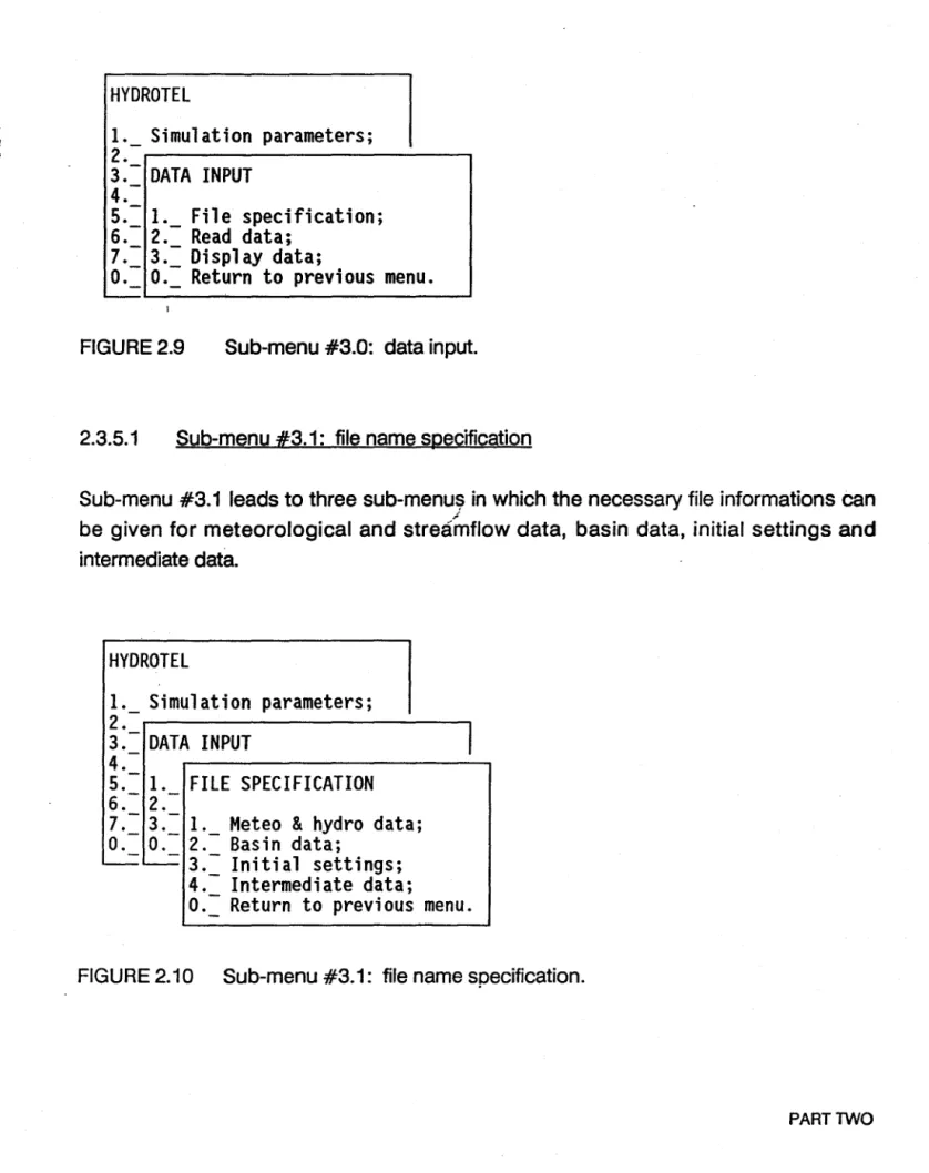
2.3.5 Sub-menu #3.0: data input

Sub-menu #3.0 (figure 2.9) leads the user to sub-menus in which he will be able to provide the informations on input data needed for the simulation.

(37)

HYDROTEL

1. Simulation parameters;

2.-r---.

3.- DATA INPUT

4.-5.= 1._ File specification;

6. 2. Read data;

7.- 3.- Display data;

0.= 0.= Return to previous menu.

'

-FIGURE 2.9 Sub-menu #3.0: data input.

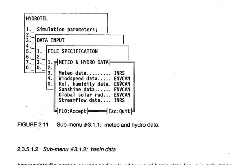
2.3.5.1 Sub-menu #3.1: file name specification

Sub-menu #3.1 leads to three sub-menu~ in which the necessary file informations can

/

be given for meteorological and streamflow data, basin data, initial settings and intermediate data.

HYDROTEl

1. Simulation parameters;

2.- 1

3.- DATA INPUT

4.-5.- 1. FILE SPECIFICATION

6.-

2.-7.- 3.- 1. Meteo

&

hydro data;

0.- 0.- 2.- Basin data;

~~

3.- Initial settings;

4.- Intermediate data;

0.= Return to previous menu.

FIGURE 2.10 Sub-menu #3.1: file name specification.

(38)

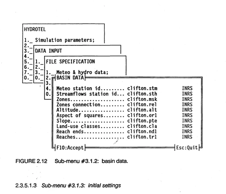
2.3.5.1.1 Sub-menu #3.1.1: meteo and hydro data

For each needed meteorological or streamflow variable, select the proper format. ; Remember that formats cannot be mixed. Ali formats used in a simulation have te be

INRS or ENVCAN or USER'S.

HYDROTEL

1._ Simulation parameters;

2. 1

3.- DATA INPUT

4.-5.- 1. FILE SPECIFICATION

6.-2.- J 1

7.= 3.=

1.

[1METEO

&

HYDRO DATA,F=====jJ

O. O. 2.

~~

3. Meteo data ... INRS

4. Windspeed data ... ENVCAN

O. Rel. humidity data. ENVCAN

~

Sunshine data ..•.•. ENVCAN

Global solar rad ... ENVCAN

Streamflow data ••.. INRS

4 FIO:AcceptlF=

=====91

Esc:Quit

FIGURE 2.11 Sub-menu #3.1.1: meteo and hydre data.

2.3.5.1.2 Sub-menu #3.1.2: basin data

Appropriate file names corresponding to ail types of basin data Iisted in sub-menu #3.1.2 (figure 2.12), together with the proper format, should appear in that window. Unless modifications are made in the source program, only INRS formats described in Appendix C should be used.

(39)

J i

HYDROTEl

INRS

9

FlO:Acceptll============I1 Esc:Quitr

FIGURE 2.12 Sub-menu #3.1.2: basin data.

2.3.5.1.3· Sub-menu #3.1.3: initial settings

Initial values can be given to variables representing the hydrological state of the basin at the beginning of the simulation. File names and proper formats are given here. Otherwise, the initial settings default to zero ("0") for surface and subsurface runoff and channel routing. In the case of the vertical budget, initial values can be also given in sub-menus #4.4.1.5 and #4.4.2.2. Informations on how to determine these initial values are given in the section on "initialization of state variables Il at the end of Part 2. See also Appendix C for structure and content of data files. Unless modifications are made in the source program, only INRS formats should be used.

(40)

( i

• HYDROTEL

1. Simulation parameters;

2.-

1

3.- DATA INPUT

4.-5. 1. FILE SPECIFICATION

6. -

2.-7.= 3.=

l'_jMeteo

&

hydro data;

0._ 0._ 2. ,INITIAl SETIINGS,t============ïl

' - - - 3.

1

4. Snowpack •.•..•. clifton.sis

INRS

O. Water budget ... clifton.pis

INRS

-- Runoff .•... clifton.ris

INRS

Streamflows .... clifton.cis

INRS

1 F10:AcceptlF

=========9IEsc:Quit~

FIGURE 2.13 Sub-menu #3.1.3: initial settings.

2.3.5.1.4 Sub-menu #3.1.4: intermediate data

Names and proper formats of the files containing intermediate data are given here (figure 2.13). See Appendix C for structure and content of data files. Unless modifications are made in the source program, only INRS formats should be used.

(41)

HYDROTEL

1._

Simulation parameters;

2.

1

3.- DATA INPUT

4.-5.-

1.

FILE SPECIFICATION

6.-

2.-7.- 3.-

1.

Meteo

&

hydro data;

0.- 0.- 2.- Basin data;

~~ 3.~Initial

settings;\

' 4. Il INTERMEDIATE DATA,I=============ïI

o.

~

Max temp ... clifton.tpx

INRS

Min temp •....•. clifton.tpn

INRS

Rain •...•....•. clifton.plu

INRS

Snow ... clifton.nei

INRS

Melt ...••... clifton.fon

INRS

Evapo ...•... clifton.evp

INRS

Outflow ... clifton.pro

INRS

Runoff ... clifton.rui

INRS

Streamflows .... clifton.deb

INRS

4 FIO:Acceptll= =========11 Esc:Quit

AGURE 2.14 Sub-menu #3.1.4: intermediate data.

2.3.5.2 Sub-menu #3.2: read data

With HYDROTEL 2.1, sub-menu #3.2 (figure 2.15) is optionaL Basin data will be read automatically, but not initial settings of the state variables.

(42)

,

j t

HYDROTEl

1. Simulation parameters;

2. -3.

_-

DATA INPUT

4. 5.:= 1._ File name specification;

6.

_-

2. -7.

_-

3.

_-

READ DATA

O.

_-

4. -O.

1.

Basin data;

' J -L...--

2.- Initial settings;

0.:= Return to previous menu.

FIGURE 2.15 Sub-menu #3.2: read data. 2.3.5.2.1 Sub-menu #3.2.1: basin data

,

"

With HYDROTEL 2.1, sub-menu #3.2:~ (figure 2.16) is optional. Data will be read automatically.

(43)

HYDROTEl

1._ Simulation parameters;

2.

-3. _-

DATA INPUT

4. -5.

1.

6.

-_-

2.

-_-

READ DATA

₁

7.

_- 3.

-O. -O.

_- _- 1.

_-

BASIN DATA

'--~

2.

J

O.

-

_-

1.

Meteo station id;

2.

-

Streamflows station id;

-

-3. _-

Zones;

4.

_-

Zone connection;

5. Altitude;

6.=: Aspect;

7._ Slope;

8. _-

Land-use classes;

9.

Reach ends;

A.= Reaches;

0._ Return to previousmenu.

FIGURE 2.16 Sub-menu #3.2.1: basin data.

2.3.5.2.2. Sub-menu #3.2.2: initial settings

With HYDROTEL 2.1, sub-menu #3.2.2 (figure 2.17) is optiona!. If the user wants to initialize the state variables with values computed in a previous run, he must select the corresponding options. Otherwise, runoff, streamflow and snowpack values will default to zero and water budget variables will have to be read at sub-menu #4.4.1.5 or #4.4.2.2.

(44)

!

•

HYDROTEl

1._ Simulation parameters;

2 . 3.- DATA INPUT 4. -5. 1. 6.- 2.- READ DATA 7.- 3.-0.- 3.-0.- 1.

--= -=

2.- INITIAL SETTINGS 1

0.--=

1. Snowpack;

2.- Water budget;

3. Runoff;

4.- Streamflows;

0.= Return to previous menu.

FIGURE 2.17 Sub-menu #3.2.2: initial settings.

2.3.5.3 Sub-menu #3.3: display data

If one wants to have a visual representation of files containing basin data, he can select options 1, to 6 in sub-menu #3.4 (figure 2.18). The selected variable will be displayed on the screen, together with an appropriate legend. If option 7 is selected sub-menu #3.3.1

(45)

HYDROTEl

1._ Simulation parameters;

2. 3.- DATA INPUT

4.

-5.- 1. File name specification;

6. 2.- Data format specification;

7.

3.-0.- 4.- DISPlAY DATA

~O.-~

1. Basin mask;

) 2.- Altitude;

3.- Aspect;

4.- Slope;

5.- Reach ends;

6.- Reaches;

7.- Streamflows, tempo

&

pree.

0.= Return to previous menu.

FIGURE- 2.18 Sub-menu #3.3: display d~ta.

2.3.5.3.1 Sub-menu #3.3.1: streamflows, tempo & prec.

Withthis menu the user can select a simulation period by diplaying the observed streamflows, temperatures and precipitations for a given year. The user selects the year he wants to look at by entering the last two digits of that year. The user can also select specifie hydrological or meteorological stations among those available by pressing the "Space" bar, once on the related field.

See figure 2.85 and related description for more details on how to use the interactive vertical window when the meteorological and streamflow data are displayed.

(46)

HYDROTEl

1. Simulation parameters;

2.-~---,

3.-

DATA INPUT

4.-5.-

1. File name specification;

6.- 2.-

Data format specification;

7. - 3 . - . . . - - - . 0.- 4.-

DISPlAY DATA

----=

0.---=

1. Basin mask;

) 2.-

Altitude;

3.-

Aspect;

4.-

Slope;

5. - Reach ends;

6.-

Reaches;

7 •

-~

STREAMFlOW, TEMP

&

PREC

:1=======iI

o.

' - Vear ... 73

Hydrological station no ... 0030242

Meteorological station no ...•. 7020885

/ ... 4/

y

FlO:Displayll=

=======11

Esc:Quit

FIGURE 2.19 Sub-menu #3.3.1: streamflows, tempo & pree ..

2.3.6 Sl,Jb-menu #4.0: sub-models

HYDROTEl

1. Simulation parameters;

2.= Optimization parameters;

3. 4.-

SUB-MODElS

5.-6.= 1._ Interpolation of precipitations;

7. 2. Snowmelt;

0.- 3.-

Evapotranspiration;

----=

4.= Vertical water budget;

5. Surface and sub-surface runoff;

6.-

Channel routing;

0.-

Return to previous menu.

(47)

Ali options (figure 2.20) can be selected by moving ta each of those options and pressing "ENTER". After typing ail necessary data, in the sub-menus corresponding ta those options return to the "main menu" by selecting option "0" and pressing "ENTER". It is possible ta Olby pass" any of the submodels. In HYDROTEL 2.1, intermediate data corresponding to the output from that sub-model has then ta be read.

The first five options applies to cells or HHU's, while channel routing is applied for the river network build up by the reaches.

1

2.3.6.1 Sub-menu #4.1: interpolation of precipitation See section 3.2 for more informations.

HYDROTEl

1. Simulation parameters;

2.= Optimization parameters;

3. 1

4.-

SUB-MODElS

5.- . 6.- 1.

INTERPOLATION OF PRECIPITATIONS

7. - 2. 0.- 3.-

1. Bypass;

~

4.- 2.- Read meteo data from disk;

5.- 3.-

Thiessen polygons;

«

6.- 4.-

Weighted mean of nearest three stations;

0.- 5.-

User's defined interpolation;

~ 6.-

Stand alone program;

0.= Return to previous menu.

FIGURE 2.21 Sub-menu #4.1: interpolation of precipitation.

Six options are available for the interpolation of precipitations (figure 2.21). Select one of those and press "ENTER". After typing the input values, retum to "sub-menu #4.0" by selecting option "0" and pressing "ENTER".

(48)

Option 1 is chosen if no output is required fram the sub-model in a particular run.

: Option 2 allows the user to read precipitation matrices obtained fram a previous run or elsewhere, for example from weather radar or satellite data. Precipitation values are read from the file specified in sub-menu #3.1.4 (intermediate data) to be used by the next sub-models. Two weil known interpolation methods are provided as options 3 and 4. It will be also possible for the user to write its own interpolation submodel (options 5 and 6), following the instructions given in Appendix 0 or E.

l

2.3.6.1.1 Sub-menu #4. 1. 1: Thiessen polygons (figure 2.26)

HYDROTEL

1._

Simulation parameters;

2._ Optimization parameters;

3. 1

4.-

SUB-MODELS

5.-6.- 1.

INTERPOLATION OF PRECIPITATIONS

7. - 2.

0.= 3.= 1._

_j

Byp ass, read data,from disk;

-

4._ 2. 1THIESSEN POLYGONS,I==============iI

5. 3.

6.=

4. Precipitation vert. grad. (%/IOOm) ... O.

0._ 5. Temperature lapse rate (C/IOOm) ... O.

- o .

-

., FlO :Accept

1

1 Esc: Quit

FIGURE 2.22 Sub-menu #4.1.1: Thiessen polygons.

Precipitation: vertical gradient (%/100 m): type the main vertical gradient of precipitations, in % per 100 meters. Type "0", if you consider that the vertical distribution of stations can take care of the gradient.

(49)

Temperature: lapse rate (OCj100 ml: type the temperature lapse rate in degrees Celcius per 100 meters. Type "0", if you consider that the vertical distribution of stations can take care of the lapse rate.

When this is done, leave the sub-menu by pressing "F10" (accept and save the new values) or "ESC" (no change to previously stored values).

2.3.6.1.2 Sub-menu #4. 1.2: weighted mean of nearest three stations

1

HYDROTEL

1._ Simulation parameters;

2._ Optimization parameters;

3. 1

4.- SUB-MODElS

5.

-6.- 1. INTERPOLATION OF PRECIPITAJIONS

7.- 2.

0.- 3.- 1. Bypass, read data from disk;

~

4.- 2.- Thiessen polygons;

5.=

3.~WEIGHTED

MEAN OF NEAREST THREE

STATIONS~~====~

6. 4.

O.~

5. Precipitation vert. grade (%/100m) ..•

o.

~

o.

Temperature lapse rate (C/100m) ... O.

'

-.

9F10:Acceptl

IEsc:Quit

FIGURE 2.23 Sub-menu #4.1.2: weighted mean of nearest three stations.

As seen in figure 2.23, this sub-menu is similar to 4.1.1. The information given in 2.3.6.1.1 applies.

(50)

2.3.6.2 Sub-menu #4.2: snowmelt

HYDROTEl

1. Simulation parameters;

2.-

Optimization parameters;

3.

4.-

SUB-MODElS

5.-6.- 1. 7 • - 2. -

SNOWMEl T

0.-

3.,--

4.:=

1._

Bypass;

5. 2. Read snowmelt data from disk;

«

6.- 3.-

Modified degree/day method;

0.- 4.-

User's defined snowmelt;

--- 5.:= Stand alone program;

0._ Return to previous menu.

FIGURE 2.24 Sub-menu #4.2: snowmelt.

l

/

Rve options are currently available for snowcover simulation and melting (figure 2.24). Select one and press "ENTER".

..

Option is·chosen if no output is required fram the sub-model in a particular rune

Option 2 allows the user to read melt water matrices obtained fram a previous run or elsewhere. For instance, melt values derived fram passive microwave data could be read here. Values are read fram the file specified in sub-menu #3.1.4 (intermediate data) ta be used by the next sub-models. A modified degree-day method is pravided as option 3. It will be al 50 possible for the user ta write its own snowmelt subprograms (options 4 and 5), following the instructions given in Appendix DorE.

(51)

1

•

2.3.6.2.1 Sub-menu #4.2.1: modified degree-day method (figure 2.29)

HYDROTEL

1._ Simulation parameters;

2._

Optimization parameters;

3.

-4.

_-

SUB-MODELS

5.

-6. _- l.

-7.

2.

SNOWMELT

o.

-

3.,

-' - - -

4.

_1.

5.- 2.-

_{MODIFIED DEGREE/DAY METHOD}

6. _- 3.

-o.

_-

4.

1.

Parameters;

0.- 2.=

Land-use groups;

'

--

3.

Optimization parameters;

,-0.=

Return to previous menu.

FIGURE 2.25 Sub-menu #4.2.1: modifiéd degree-day method.

Sub-menu #4.2.1 (figure 2.25) is essentially an intermediate menu. Option 1 "paraméters", gives access to the menu in which values of the parameters of the

snowmel~ sub-model are determined. Option 2, "land-use groups", allows integration of

original land-use groups to suit the sub-model. Option 3, "optimization parameters· gives access to the menu in which the value of the optimization parameter related to the modified degree-day method can be initialized.

(52)

J

2.3.6.2.1.1 Sub-menu #4.2.1.1: parameters (figure 2.30)

HYDROTEl

1. Simulation parameters;

2.= Optimization parameters;

3.

4.-

SUB-MODElS

5.-6.- l.

7.- 2.-

SNOWMElT

0.- 3.'-~ 4.- l.

5.= 2.=

MODJFIED

DEGRE~/DAY

METHOD

6._ 3._

nPARAMETERS.I==================iI

O. 4. 1.

---- 0.- 2. Temp. for transfo of rain into snow (OC) .... O.

~

3. Melt factor (coniferous forest) (mm/dOC) •..• 2.

O. Melt factor (deciduous forest) (mm/dOC) ....• 3.

~

Melt factor (open areas) {mm/dOC} .•... 4.

Threshold tempo for melt (OC) ••.•.•.•..•...• O.

Melt rate at snow/,ground interface (mm/d) ... 0.5

Maximum density of snowpack (kg/m3} ... 550

Settlement constant. .•.••..•.•..•.•.•....•.. 0.1

4 FlO :Accept

1 1

Esc:Quit

~

FIGURE 2~26 Sub-menu #4.2.1.1: parameters.

See section 3.3 for more informations.

Temperature for transformation of rain into snow (OC): type the threshold temperature (OC) for the transformation of rain into snow.

Melt factor (coniferous forest) (mmjd-OC): type melt factor for coniferous forests. in millimeters per day and degree Celcius.

Melt factor (deciduous forest) (mmjd-OC): type melt factor for deciduous forests; Melt factor (open areas) (mmjd-OC): type melt factor for open areas.

(53)

f

j

J

Threshold temperature for melt (OC): type threshold temperature for melt, in degrees Celcius.

Melt rate at snow/ground interface (mm/d): type estimated mean constant melt rate at snow/ground interface, in millimeters per day.

Maximum density of snowpack (kg/m3

): type estimated maximum density of

snowp'ack, in kilograms per cubic meters. ₁

Settlement constant: type the settlement constant (smaller than one) of the

snowp~ck.

When this is done, leave the sub-menu by pressing "F10" (accept and save the new values) or "ESC" (no change to previously stored values).

2.3.6.2.1.2 Sub-menu #4.2.1.2: land-use groups

Land-use groups corresponding to the types of land-uses needed in the snowmelt sub-model are defined in sub-menu #4.2.1.2 (figure 2.27). Three land-use groups are considerèd for snowmelt, namely: coniferous forest, deciduous or broad-Ieaved fore st and open areas.

(54)

HYDROTEL

i

1. Simulation parameters;

J

2.- Optimization parameters;

3.-r---~

4.-

SUB-MODELS

5.-6.- l.

7.- 2.-

SNOWMELT

0.- 3.-~ 4.- 1. 1

5.: 2.= MODIFIED DEGREE/DAY METHOD

CLASS CODE (SEPARATED BY

"+")

FOR CONIFEROUS FOREST

RESIN

CLASS CODE (SEPARATED BY

"+")

FOR BROAD-LEAVED FOREST

~_.r·

FEUIL

FIGURE 2.27 Sub-menu #4.2.1.2: land-use groups.

As required in the menu, type the class codees) of the land-use class(es) corresponding to "coniferous forest", separated bya "+" signe Then, press "ENTER" to proceed to the next group "broad-Ieaved forest". Again, type the class codees) corresponding to "broad-Ieaved forest" and press "RETURN". The original land-use classes that have not been assigned to either "coniferous" or "broad-Ieaved" forest, are assigned automatically to "open areas".

2.3.6.2.1.3 Sub-menu #4.2.1.3: optimization parameters

ln sub-menu #4.2.1.3 "optimization parameters" (figure 2.28) the user can set initial values and limits for the parameters ta vary within. When the field "state" is ON the

(55)

optimization process will consider. this variable. If "state" is OFF, the variable will be ignored. The other three fields "minimum", "initial" and "maximumu

are related to a coefficient multiplying the melt factors (sub-menu #4.2.1.1): "initial" is the initial value of

, the coefficient, "minimum" is the lower limit on the coefficient and "maximum- is the upper limit on the same coefficient.

HYDROTEL

1.

S~mulation

parameters;

2.- Optimization parameters;

3.-4.- SUB-MODELS

5.-6. - 1.

7.- 2.-

SNOWMELT

0.- 3.-' - - 4.- 1.

5.- 2.-

MODIFIED DEGREE/DAY METHOD

6. 3. ~

0.-

4.- 1. Parameters;

~ 0.- 2.-

Land-use groups;

-

3.-~OPTIMIZATION

PARAMETERS:I==========::;'I

o.

~

state

minimum

initial

maximum

Melt factor

ON

O.

1.

100

~FlO:Acceptl=l

==========4IEsc:Quitr

FIGURE 2.28 Sub-menu #4.2.1.3: optimization parameters.

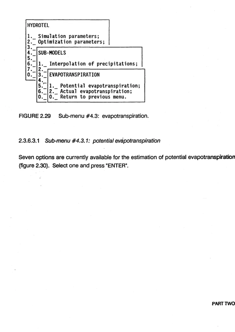
2.3.6.3 Sub-menu #4.3: evapotranspiration

ln HYDROTEL 2.1, the user is allowed to choose between formulae for the determination of potential or actual evapotranspiration (figure 2.29). A few options are offered so as to make use of available data. Select option 1 or 2 to have access to the sub-menus containing the options. Note that potential or actual evapotranspiration data will be saved in intermediate data files depending on the option chosen here.