2D½ THERMAL-MECHANICAL MODEL
OF CONTINUOUS CASTING OF STEEL
USING FINITE ELEMENT METHOD
–
Modèle thermo-mécanique 2D½
de la coulée continue de l’acier
à l’aide de la méthode des éléments finis
Thèse présentée en vue de l’obtention du grade de
Docteur en Sciences Appliquées
par Frédéric Pascon
Année académique 2002-2003
Faculté des Sciences Appliquées Génie Civil et Géologie
Département de Mécanique des matériaux et Structures Secteur Mécanique des Solides et des Matériaux
Membres du Jury : J. Lecomte-Beckers
Chargée de cours Université de Liège, présidente du jury S. Cescotto
Professeur Université de Liège A. M. Habraken
Maître de recherches FNRS à l’Université de Liège, promoteur M. Bellet
Maître de recherche CNRS à l’Ecole des Mines de Paris (France) B.G. Thomas
Professeur University of Illinois at Urbana-Champaign (USA) H. Grober
Directeur Innovation, Recherche & Développement, Profil ARBED, Groupe Arcelor L. Chefneux
Directeur Stratégie et Progrès Technique, Cockerill-Sambre, Groupe Arcelor M. Bobadilla
Chef du Service Transformation de phase et précipitation, IRSID, Groupe Arcelor
Coordonnées de l’auteur : Pascon Frédéric
Département M&S
Université de Liège
1, chemin des Chevreuils
4000 Liège
Belgique
Foreword
This work has been possible thanks to a significant collaboration between M&S Department and R&D teams within steel making industry: Profil Arbed Research and Direction du Développement Technique of Arcelor Group.
I would like to express my gratitude to everyone who helped me making this work interesting and especially Mrs Habraken for her advice in the thesis writing.
Today, I also have a though to my nearest and dearest who always supported me and encouraged.
i
Contents
I. INTRODUCTION ... 1
1. FUNDAMENTALS OF CONTINUOUS CASTING PROCESS... 1
1.1. Historical and industrial context ... 1
1.2. Phenomenology and terminology of continuous casting... 2
2. INDUSTRIAL OBJECTIVES OF THE MODEL... 8
2.1. Thermo-mechanical model of continuous casting in the mould region ... 8
2.2. Prediction of the risk level in transverse cracks formation during bending and straightening of steel slabs. Study of the influence of some local defects. ... 9
3. MAIN FEATURES OF THE MODEL... 9
3.1. General approach: 2D½ slice model... 9
3.2. Thermo-mechanical finite element method ... 10
4. OUTLINE OF THIS THESIS... 10
5. ORIGINAL CONTRIBUTION OF THIS THESIS... 11
II. THERMAL MODEL ... 15
1. SOLIDIFICATION OF ALLOYS AND STEEL... 15
1.1. Crystalline structure ... 15
1.2. Solid solutions... 17
1.3. Phase diagrams... 17
1.3.1. Pure materials...17
1.3.2. Complete solid solutions ...19
1.3.3. Eutectic diagram without solid solution ...21
1.3.4. Eutectic diagram with limited solid solution ...21
1.3.5. Eutectoid diagram...22
1.3.6. Peritectic diagram...23
1.3.7. Fe-Fe3C phase diagram...23
1.4. The lever rule ... 25
1.5. Steel compostion during solidification: examples... 27
1.6. TTT diagrams... 31
1.7. Assumptions in the model... 32
2. COEFFICIENT OF THERMAL LINEAR EXPANSION... 33
3. INTERNAL HEAT CONDUCTION... 35
4. THERMAL BOUNDARY CONDITIONS... 37
III. MECHANICAL MODEL ... 41
1. GENERALIZED PLANE STRAIN STATE... 41
1.1. Principle ... 41
1.2. Bending and straightening using generalized plane strain state ... 42
1.3. Application of extracting force ... 45
1.3.1. Origin of extracting force ...45
1.3.2. Extracting force, extracting rolls and distribution of work ...47
1.4. Neutral axis... 49
2D½ thermal-mechanical model of continuous casting using finite element method
ii
2.1. Decomposition of total strain...50
2.1.1. Thermal and phase transformation strains... 50
2.1.2. Mechanical strains ... 51
2.2. Elastic domain...51
2.2.1. Hooke’s law for isotropic materials ... 51
2.2.2. Time integration of Hooke’s law with temperature dependence... 52
2.3. Viscoplastic domain ...55
2.3.1. Basics of theory of plasticity... 55
2.3.2. Yield locus: elasticity/plasticity criterion... 56
2.3.3. Plastic flow rule (large strains) ... 61
2.3.4. Plastic flow rule associated to Von Mises criterion ... 63
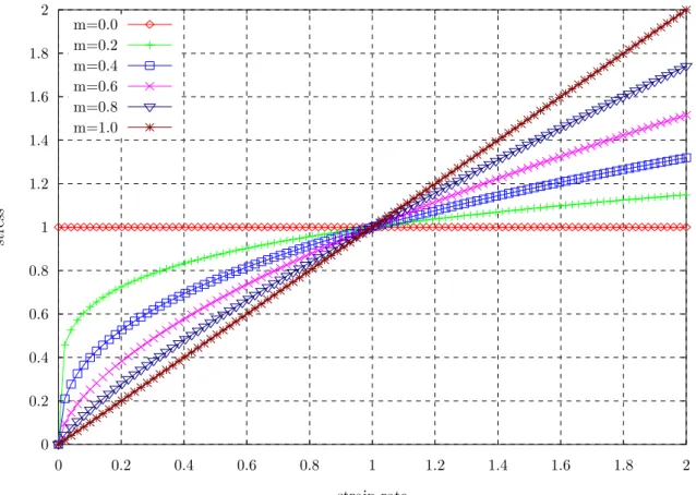
2.3.5. Viscoplastic behaviour of steel at high temperature: Norton-Hoff law... 64
2.3.6. Modification of Norton-Hoff law... 68
2.3.7. Implicit time integration of modified Norton-Hoff law ... 71
2.3.8. Analytical compliance matrix ... 76
2.4. From elasticity to viscoplasticy: yield limit...51
2.5. Loading/unloading criterion ...78
2.5.1. First example: without thermal effect ... 78
2.5.2. Second example: including thermal effect ... 79
2.6. Analytical vs. numerical verification : study of a small cylinder ...79
3. FERROSTATIC PRESSURE...80
4. MECHANICAL CONTACT...83
4.1. Phenomenology and general aspects ...83
4.1.1. Local and global approaches... 83
4.1.2. Notations... 84
4.1.3. Unilateral contact... 86
4.2. Some usual constitutive contact laws ...88
4.2.1. Coulomb’s model... 88
4.2.2. Orowan model ... 89
4.2.3. Tresca’s model... 89
4.2.4. Viscoplastic models: Norton-Hoff model ... 90
4.3. Penalty technique...90
4.4. Contact element...96
4.4.1. Distance between the solid and the foundation ... 97
4.4.2. Virtual work... 98
4.4.3. Gauss integration ... 99
4.5. Stiffness matrix...99
IV. THERMAL-MECHANICAL COUPLING: STAGGERED ANALYSIS ...103
V. 1ST INDUSTRIAL APPLICATION: MODELLING OF A 125MM SQUARE BILLET IN THE MOULD REGION. EFFECT OF THE MOULD TAPER...107
1. DEFINITION OF THE PROBLEM...107
1.1. Context of the study...107
1.2. Importance of the mould taper ...107
2D½ thermal-mechanical model of continuous casting using finite element method
iii
1.4. Thermal parameters... 110
1.4.1. Initial conditions...110
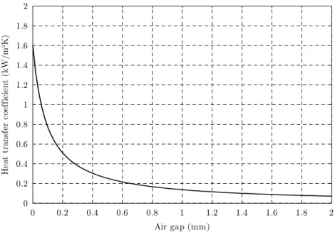
1.4.2. Heat transfer coefficient ...110
1.4.3. Thermal linear expansion coefficient ...112
1.5. Mechanical parameters ... 112
1.6. Modelling of the liquid behaviour... 112
2. RESULTS... 113
2.1. Idealised mould... 113
2.1.1. Billet distortion...114
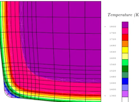
2.1.2. Thickness of solidified shell and temperature at the exit of the mould...115
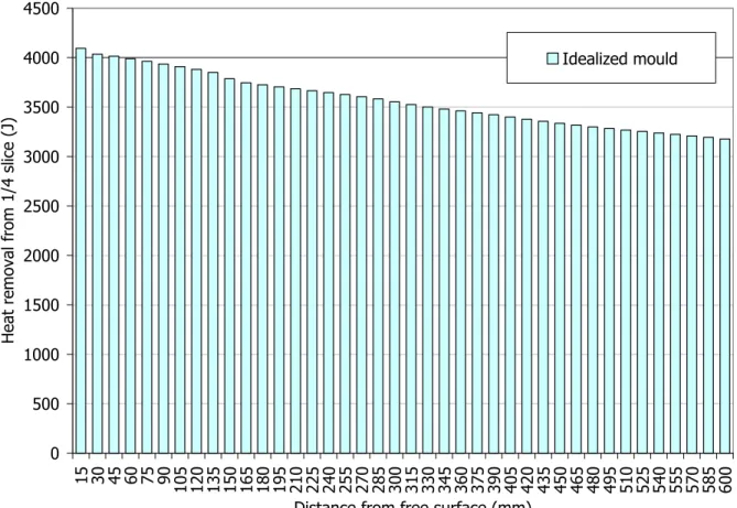
2.1.3. Heat removal from the ¼ slice...117
2.2. Real mould ... 117
2.2.1. Heat removal from the ¼ slice...117
2.2.2. Thickness of solidified shell and temperature at the exit of the mould...119
2.2.3. Mechanical state of the billet...122
2.3. To an automatic optimization of mould taper ... 123
2.4. Mould distortion ... 124
3. DISCUSSION... 127
VI. 2ND INDUSTRIAL APPLICATION: EVALUATION OF RISK OF TRANSVERSE CRACKING DURING BENDING AND STRAIGHTENING OF STEEL SLABS & INFLUENCE OF SOME LOCAL DEFECTS ... 131
1. GEOMETRY OF THE PROBLEM... 131
1.1. Cast product... 131
1.2. Caster geometry... 132
1.2.1. Radius of curvature ...132
1.2.2. Rolls geometry ...132
1.2.3. Water spray cooling...133
2. THERMAL AND MECHANICAL PARAMETERS... 135
2.1. Steel grade and material properties... 135
2.2. Bulging control ... 136
2.2.1. Bulging with slice models ...136
2.2.2. Bulging based on elastic plates theory...138
2.2.3. Extension of the method...143
2.3. Extraction force ... 144
2.3.1. Evaluation of extraction force: coupled approach ...144
2.3.2. Curves of extraction force from the caster manufacturer: uncoupled approach...145
2.3.3. Which curve to use? ...147
2.3.4. Weight of the slab...148
2.4. Definition of indexes relative to risk of transverse cracking... 149
2.5. Modelling of the liquid behaviour... 150
3. REFERENCE CASE: CASTING IN STANDARD CONDITIONS – NO LOCAL DEFECT... 150
3.1. Initial conditions ... 150
3.2. Evolution of the slab surface temperature ... 150
2D½ thermal-mechanical model of continuous casting using finite element method
iv
3.4. Indexes of transversal cracking...159
3.5. Reference case in bending zone ...159
4. COMPARATIVE STUDY OF LOCAL DEFECTS...166
4.1. Partial blockage of nozzles: local reduction of cooling rate...166
4.1.1. Definition of the local defect ... 166
4.1.2. Effect on the surface temperature ... 166
4.1.3. Effect on thickness of the slice... 166
4.1.4. Effect on risk of transverse cracking... 167
4.1.5. Conclusion ... 167
4.2. Locking of pairs of rolls ...174
4.2.1. Definition of the local defect ... 174
4.2.2. Effect on the surface temperature ... 177
4.2.3. Effect on thickness of the slice... 177
4.2.4. Effect on risk of transverse cracking... 178
4.3. Misalignment of one pair of rolls...182
4.3.1. Definition of the local defect ... 182
4.3.2. Effect on the surface temperature ... 185
4.3.3. Effect on thickness of the slice... 185
4.3.4. Effect on risk of transverse cracking... 185
5. DISCUSSION...191
VII. CONCLUSION AND PERSPECTIVES...193
VIII. APPENDIX: ANALYTICAL DEVELOPMENTS...197
1. IMPLICIT TIME INTEGRATION OF NORTON-HOFF LAW...197
2. ANALYTICAL COMPLIANCE MATRIX...202
I
1
I
I
I
.
.
.
I
I
I
n
n
n
t
t
t
r
r
r
o
o
o
d
d
d
u
u
u
c
c
c
t
t
t
i
i
i
o
o
o
n
n
n
1. Fundamentals of continuous casting process
1.1. Historical and industrial context
irst steps in continuous casting go back to the middle of the 19th century
[WOL00], when twin-roll casting has been developed by Sir Henry Bessemer as an alternative to ingot casting of nonferrous metals (Cu and Cu–alloys, 1843) as well as for steel casting a few years later (1856). Progressively and during about one hundred years, different modifications have been brought to the process in order to make it more efficient, accurate and economic and to improve the quality of the cast products.
The real takeoff of continuous casting in steel industry took place in the years sixty and seventy, first in Japan [MIY01] and some other countries such as Finland [TEK90] (even if the contribution of this country to the world production is marginal), then in other Western-Europe countries (West Germany, Great Britain, …) and finally in United States during the eighties. The reason of this difference between countries is linked to the technical and economical situation of each one. The worldwide 1973 petroleum crisis led occidental countries to face up to some economical difficulties: rising of energy cost, decreasing of economical activity and successive periods of recession. In this new context, steel producers had to change their politics of development in order to remain present on the international scene and to avoid an economical downfall. From the second part of the seventies up to today, steel makers have restructured many times their activity in order to reduce costs (energy, manpower savings) and to maximize yield and quality of the products. Progressively, continuous casting of steel became the chosen way to produce crude steel because this process helps to reach the economical and technical goals above. Little by little, it has effectively replaced the older ingot casting process, which is only used nowadays for very special applications.
Like any other industrial process, continuous casting has required (and shall required) for a long time tuning, development and improvement to cure cast products of defects under some difficult casting conditions, as well as to optimise the process to reach ever higher yields. The model presented in this thesis is obviously not a global
F
2D½ thermal-mechanical model of continuous casting using finite element method
2
solution. However it could contribute to go a little further in the understanding of the steel behaviour during continuous casting.
1.2. Phenomenology and terminology of continuous casting
In the production of steel, continuous casting takes place after steel making and before hot rolling. It rests on a rather simple principle: it is a kind of big “heat exchanger” which handles the continuous cooling and solidification of steel. The Figure 1 is a sketch of steel making.
Figure 1: Sketch of steel making [ARC]
OXYGEN ARGON IRON ORE COAL SINTERING COKE OVEN COKE SINTERED ORE BLAST FURNACE PIG IRON (1400°C) OXYGEN CONVERTER CRUDE STEEL CRUDE STEEL ELECTRIC ARC FURNACE GRADED LIQUID STEEL VACUUM ADDITIVES REFINING UNIT (LADLE FURNACE) CONTINUOUS CASTING OF LONG PRODUCTS CONTINUOUS CASTING OF FLAT PRODUCTS SLABS BILLETS / BLOOMS BEAM BLANKS STEEL SHEETS (COILS) BEAMS, SHEET PILES, REINFORCEMENT BARS, WIRE RODS HOT ROLLING HOT ROLLING REHEATING FURNACE (800°C-1200°C) REHEATING FURNACE (800°C-1200°C) SCRAP
2D½ thermal-mechanical model of continuous casting using finite element method
3
Basically, there are two different ways to produce crude steel:
1. In the first one (called smelting process), iron ore is prepared and crushed (in the sintering plant), while coal is distilled into coke (a powerful combustible, very rich in carbon). Then, the blast furnace is filled by successive layers of sintered ore and coke, while hot air (1200 °C) is blown at the bottom causing the coke to combust. The formed carbon oxides reduce the iron oxides, and thus separate iron. At the bottom of the blast furnace, an iron-based molten mixture called pig iron is obtained together with slag (which floats on pig iron because of its lower density). Pig iron is then poured onto a bed of scrap in the bottom of a giant vat. Then, it is heated at 1600°C while pure oxygen is blown in, causing unwanted elements (carbon and residues) to burn. The obtained liquid steel is called crude steel.
2. In the second way (called electric process), scrap is molten in a large furnace thanks to powerful electric arcs between electrodes. The residue is also crude steel. Crude steel is steel, however it has to be refined by adjusting the carbon, residues and other additives content. This operation is performed in the refining unit under strongly controlled conditions: vacuum, high precision in chemical composition (steel grade). Even the temperature of graded liquid steel is highly controlled before and during its transportation to the next step: the continuous casting mill.
The Figure 2 shows the main elements of continuous casting:
Figure 2: Continuous casting mill (6 parallel lines) [ARB]
Graded liquid steel comes from the refining unit in successive ladles, the content of which being poured into a tundish. The task of the tundish is multiple: it is of course
2D½ thermal-mechanical model of continuous casting using finite element method
4
a provider, but also a buffer of liquid steel (during ladle changes) for the continuous casting process. Moreover, the design of the tundish helps the inclusion separation and prevents reoxidation.
Liquid steel flows from the tundish to the mould trough a nozzle placed in the bottom of the tundish (see Figure 3). Orifices at the end of the nozzle are under the free level in the mould (meniscus). Note that the use of submerged entry nozzle is not systematic, free jet filling is also used in many cases. A special powder covers the free surface, its expected functions being [RIB79]:
• to protect the liquid steel against oxidation by contact with oxygen in the air; • to insulate the free level and to avoid partial solidification at the surface; • to absorb inclusions rising up to the surface;
• to lubricate contact between the mould and the strand;
• to allow a homogeneous thermal transfer adapted to casting conditions.
Figure 3: Filling of the mould through the nozzle [THO02]
The mould is bottomless and its internal walls are made of Cu-alloy plates or simply a Cu-alloy tube (for billet casting). An internal water-cooling circuit keeps the wall at a relatively constant and a rather low temperature range (100-200°C) during casting.
2D½ thermal-mechanical model of continuous casting using finite element method
5
When liquid steel comes in contact with cold walls of the mould, it freezes and a solidified shell starts to form all around the perimeter of the cast product. Then, the solid shell is growing to the core.
At the same time, some extracting rolls are pulling out the forming steel strand, which is thus moving downward, and the mould must be supplied in liquid steel to insure a continuous process and a constant level in the mould. The velocity of the strand is called casting speed.
Considering a horizontal slice moving downward the mould, three areas can be recognized:
• the external solidified layer; • the liquid core;
• an intermediate zone, partly made of liquid and solid fractions, called mushy zone. While the slice is in progress in the mould, the solid shell is growing and it must be thick and strong enough when the slice reaches the exit at the bottom of the mould. Otherwise, some obvious problems occur such as cracks or even breakout (the liquid steel flows through the pierced shell). So the mould must extract heat from the steel at a maximum rate, allowing the solidification to reach the highest possible depth inside the strand.
To avoid the thin and fragile solid shell to stick to mould walls, which can causes cracks, a lubricant agent is usually contained in the powder. When the powder smelts in contact with steel, it forms a viscous film that flows in thin layer between the strand and the mould walls. So, there is an effective consumption of powder, which also requires a continuous providing.
In parallel to the use of lubricant powders, sticking is avoided thank to vertical oscillation of the mould. A consequence of vertical oscillation is the formation of oscillations marks at the surface of the product. These oscillation marks remain visible on the surface of the cast product. They look like short waves the frequency of which corresponds to the frequency of the mould oscillation. Moreover, they represent singularities from where transverse cracks generally initiate, even later during casting. Formation of oscillation marks is more detailed in some relevant publications [MAH91b,BRE93,BRI93].
Beneath the mould, the heat removal from the strand continues thanks to water sprays. This part is called secondary cooling as opposed to cooling in the mould region, called primary cooling. Nozzles are spraying the surface of the strand with either straight water or air mist (air + water), which is used more and more (less blocage, more uniform coverage, but more expensive [JES86,PAT00]). Globally, the temperature decreases not only at the surface, but also in the strand. The solidified shell grows until it reaches the middle of the strand. Then, the liquid pool, which is contained in the solid envelop, is closed (see Figure 4).
As long as the liquid pool is not completely closed, the liquid core of the strand is under pressure. The height of fluid column in the pool becomes in fact considerable (several meters) and a hydrostatic-type pressure is present everywhere in the liquid
2D½ thermal-mechanical model of continuous casting using finite element method
6
steel: this is the ferrostatic pressure. This pressure is applied by the pool onto the solidified shell, which tends to inflate, just like a pressurized tube.
Figure 4: Closing of liquid pool: the metallurgical length
Secondary cooling being slower than primary one, the liquid pool is closing rather far from the bottom of the mould. Usually, when the section is completely solidified, a typical length of the strand is between 15 and 25 meters, depending on the product and the casting conditions. To avoid the development of too large ferrostatic pressure, it is necessary to limit the height of the fluid column. To do so, the steel strand is brought to a horizontal position: the strand should be bent and then straightened. They are two main ways to generate a bent strand: the first one is literally to bend a straight strand. This can be realised using rolls, the function of which being to guide and support the steel strand during its advance through the machine. In such a case the caster is qualified as vertical-curved machine, since the first part of the strand (and the mould particularly) is vertical. The second way to generate a bent strand is to use a curved mould so that the strand is directly solidifying with a constant curvature. Then only straightening operation is necessary. Such a caster is qualified as curved machine. Several types of caster exist: the Figure 5 illustrates the 5 main types of casters. Whatever the type of the caster is, the position of the rolls imposes the path followed by steel and it is possible this way to bend and straighten it.
2D½ thermal-mechanical model of continuous casting using finite element method
7
Bending and straightening are rather delicate operations because of flexional stresses introduced in the material by this way:
• during bending: longitudinal tensile stress on extrados face and compression stress on intrados face of the strand (i.e. along casting axis)
• during straightening : longitudinal compression stress on extrados face and tensile stress on intrados face of the strand
Figure 6: Longitudinal stresses during bending and straightening
These longitudinal tensile stresses, combined to transverse oscillation marks and low ductility of steel in a given range of temperature, maximize the risk of transverse cracks formation on surface of the cast product. The combination of all these conditions is particularly present on the intrados face during straightening.
Some rolls are motorised so that the strand can be extracted thanks to the transmission of an “extraction force” by friction between these extracting rolls and the surface of the product. The electrical motors are supplied in such a way that the speed of the strand in the machine (“casting speed”) is regulated and generally constant (except in case of transition between successive heats cast).
Another effect of the rolls is to limit the bulging of the solid shell under ferrostatic pressure. In fact, the strand must pass through each pair of rolls and the gap d left between the rolls imposes the maximum thickness of the product at a given position in the caster. The shape of the strand (and its bulging) is thus similar to Figure 7.
2D½ thermal-mechanical model of continuous casting using finite element method
8
Without extracting rolls, the strand would not exit from the caster because the weight of the product is insufficient to overcome resisting forces, that is to say bending and straightening efforts as well as frictional effort of rolls spinning around their axis, even with ball bearing (low friction – theoretically).
One benefit of continuous casting is to provide to the product a shape close to the final section of the product. It is in fact very interesting to cast and to model the hot product which remains much malleable. For example, to produce flat products such as steel sheets, the cast product presents a rather wide rectangular section and it is called “slab”. On the other hand, for long products such as beams or wires, the shape of the cast product is generally rectangular but closer to (or even) a square, the section of which can be large (“blooms”) or smaller (“billets”). For “I-beams”, it even exist a cast product called “beam blank” the cross section of which already being a I-shape allowing to reduce the number of passes during rolling.
2. Industrial objectives of the model
2.1. Thermo-mechanical model of continuous casting in the mould
region
In a larger framework of a European Coal and Steel Community Steel Research Program, a steel producer ProfilARBED asked to M&S Department (MSM sector) of University of Liège to develop a continuous casting model. The purpose was to provide a coupled thermo-mechanical 2D analysis for a slice perpendicular to the strand axis. This slice moves downwards in the mould and the thickening of the shell is studied during its progression. From a mechanical point of view, this slice is in a generalized plane strain state, considering double symmetry and a rigid mould at constant temperature. The geometry of the mould is adapted as the slice is moving through the mould to take into account the mould taper. The thermal exchange conditions are also modified, depending on the contact between the strand and the mould.
The following numerical tools have been developed:
• A thermo-mechanical constitutive law for solidified steel, valid for a range of temperature going from the melting point to around 800°C (to completely cover the range of temperature observed during primary cooling). Because of strain rate sensitivity of steel at this very high range of temperature, an elasto-viscoplastic Norton-Hoff law has been chosen, developed and implemented in the finite element code LAGAMINE. This law also allows the degeneration of the law to represent, in a simple manner, the behaviour of the mushy and the liquid zones. • The integration in a 2D thermo-mechanical finite element of
! heat conduction; ! solidification; ! thermal expansion; ! ferrostatic pressure;
2D½ thermal-mechanical model of continuous casting using finite element method
9
! energy dissipated by plastic deformation.
• A unilateral contact element which manages the contact and loss of contact and the resulting variations in thermal exchange rates, as well as friction in the vertical movement of the strand and the resulting resistance to withdrawal.
• A mobile boundary element which models the mould taper.
• An efficient numerical strategy for the global resolution of the coupled thermo-mechanical problem: a staggered approach which allows different thermal and mechanical time steps.
Many parameters were available from data collection of the industrial partner and supplied for thermal and mechanical constitutive laws. However, parameters of the Norton-Hoff type law have been fit on experimental curves performed on a Gleeble device. The specific developments for this application are detailed in chapter V.
2.2. Prediction of the risk level in transverse cracks formation during
bending and straightening of steel slabs. Study of the influence of
some local defects.
After having developed the above first application, another steel producer contacted M&S Department for an extension of the model to the secondary cooling of the continuous casting process. In fact, under some conditions, transverse off-corner cracks were observed on continuously cast slabs. The mechanism of transverse cracking was already well known. Among others parameters, some local defects in caster can lead to the formation of this kind of transverse cracks: cooling rate defect, roll locking or roll misalignment are examples of such defects.
The purpose of the study was not to determine if these defects can generate such transverse cracks, but to attempt to classify them from the most critical to the less one in terms of risk of cracks formation. To do so, it has been necessary to define indexes which allow comparing each defect with the others.
Since the most critical zone of the caster is the straightening, almost the complete caster has been modelled, the temperature, stress and strain histories being essential for the study. The model is still based on the slice in generalized plane strain state. All details are available in chapter VI.
3. Main features of the model
3.1. General approach: 2D½ slice model
The model is based on a coupled thermal and mechanical analysis using finite element method. From initial settings, a complete three-dimensional analysis has seemed unworkable, because of numerical stability and convergence reasons, but also CPU cost. A so-called “2D½” approach has been preferred, taking advantage of the “generalized plane strain state” (see section III.1).
This approach consists in modelling a thin slice of the steel strand, perpendicular to the casting direction. Assuming a constant casting speed, time scale is equivalent to the position of the slice in the caster along the casting axis, the scale factor precisely being the casting speed.
2D½ thermal-mechanical model of continuous casting using finite element method
10
The model allows studying thermal and mechanical evolution of the slice during its advance through the caster, including heat transfer, solidification, thermal shrinkage, stress development, ferrostatic pressure, control of bulging and application to the slab of extracting force.
Placing one after the other the successive results of the studied slice, a three-dimensional view of the process in steady-state conditions can be reproduced.
3.2. Thermo-mechanical finite element method
Nowadays, the finite element method has become a usual way to solve many physical problems. Many publications introduce and develop this method [ZIE00,RAP98], so that its general principles are assumed to be known and not reminded here.
The present model is implemented in the LAGAMINE non-linear finite element code, which has been developed at M&S Department of University of Liège since early eighties [GRO85,CES89,HAB01]. Since it is dedicated to solid mechanics modelling, LAGAMINE has been written in updated material (lagrangian) formalism. No fluid flow is thus modelled: molten steel is only present in the model to provide matter to solidify and to apply ferrostatic pressure).
Many applications and theses contributed to the development of the code up to its current state: among others, modelling of forging, rolling, deep drawing processes. The large displacements and large strains formalism has been detailed by Charlier [CHA87]. Cescotto, Charlier and Habraken developed the thermo-mechanical contact element [CHA90,HAB98b]. The thermo-mechanical coupling has been studied by Habraken in her Ph.D. thesis as well as phase transformations [HAB89,HAB92]. The generalized plane strain state has been introduced by Bourdouxhe [BOU86] and also used with shell elements in the Ph.D. thesis of Grisard [GRI93].
4. Outline of this thesis
This thesis is introducing first the theoretical developments necessary to model thermal and mechanical behaviour of the steel during continuous casting. After this introductive chapter, two chapters are dedicated to these topics.
In Chapter II, thermal behaviour and equations are presented. It includes a first section describing the solidification of steel and phase transformations, since this topic is fundamental in the description of the material behaviour. This metallurgical description has been introduced in the thermal model chapter because the primary parameter guiding solidification is the temperature. After that, thermal expansion is introduced, followed by internal conduction and thermal boundary conditions.
In Chapter III, dedicated to mechanical part of model, the generalized plane strain state is introduced and the way to use it in continuous casting modelling is developed: modelling of bending/straightening, application of an extraction force, determination of neutral axis. After that, the mechanical constitutive law is described. A unified elastic-viscoplastic constitutive law for steel at high temperature (solid as well as liquid) is proposed. The elastic domain is first introduced and then the viscoplastic domain. After that, the problem of determination of yield limit is presented as well as the loading/unloading criterion. Finally, some examples are
2D½ thermal-mechanical model of continuous casting using finite element method
11
presented. The analytical developments in the time integration of the viscoplastic law and in the stiffness matrix determination are reported in an appendix at the end of the thesis. After the constitutive law, the ferrostatic pressure element and the main assumptions involved in this pressure application are introduced. Finally, this chapter ends with the description of the thermo-mechanical contact element.
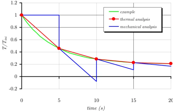
The Chapter IV is dedicated to the coupling between thermal and mechanical behaviour and the numerical problems linked to the spatiotemporal discretization. The staggered time-stepping scheme used in the present model is described.
After having developed all these theoretical topics, the two industrial applications introduced above (see section I.2) are detailed in two separated chapter.
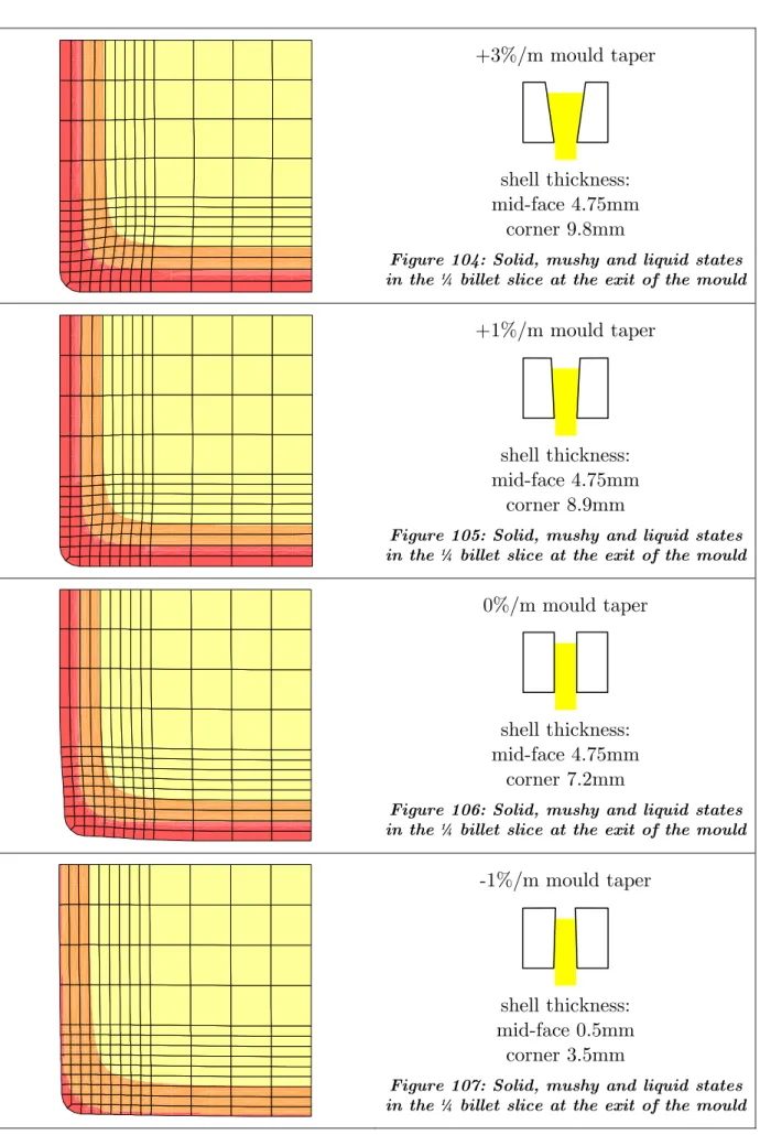
In the Chapter V, the application of the model to a 125mm square billet is illustrated by some results. The study of an idealized mould is first presented and then a comparison of the billet behaviour with five different single tapered moulds is presented to underline the importance of the mould taper on the thermal and mechanical states of the billet.
In the Chapter VI, the model is applied to the second industrial application. In that context, some additional features have been adopted to take into account:
• the large amount of data concerning the heat transfer coefficients; • the control of the bulging in a 2D½ slice model such the present one; • the problem of the extracting force.
Two indexes of risk of transverse cracking are also introduced, before thermal and mechanical results are illustrated for a first reference case and then for three cases including some local defects in the caster.
To conclude, the Chapter VII summarizes what can be said at the present time about the work done up till now and it gives some perspectives for future developments.
5. Original contribution of this thesis
Many continuous casting models have been developed over the last twenty-five years. One must mentioned the team of J.K. Brimacombe of University of British Columbia who settled with his collaborators the bases of finite element modelling of continuous casting. Numerous publications of his team still remain of relevant interest today, on process decription, experimental measurements and modelling as well [BRI73, MAH91a,BAK93,DIP86,BRE93,CHA93,BRI93].
The work done by B.G. Thomas, first in the above team, then with his own team in the recent years at University of Illinois at Urbana-Champain, also represents a precious contribution to the subject with many publications and thesis [STO90, MOI93a, ZHU96, YU00]. This team has developed different models, from quite simple spreadsheet model [THO91] to more complex finite element ones, which take into account thermal, mechanical, fluid flow and phase changes aspects. These models place them in a good position among the continuous casting modellers, the current “CON2D” model being the fruit of one decade in thermal-mechanical modelling [LI03].
2D½ thermal-mechanical model of continuous casting using finite element method
12
Many others teams have been working on the subject and related subject. Note that beside finite element and finite difference models, some analytical models have also been developed by mathematicians, especially at University of Jyväskylä (Finland) [LAI89,MAN90]
Before numerical modelling, the empirical knowledge of the process combined to experiments allowed improving the casting parameters and they remain important ways of investigation to better understand which are the parameters governing the process. One can not neglect the work done by the research and development teams in the industry and by the caster manufacturers (among others: IRSID for Arcelor Group, CRM in Belgium, Voest-Alpine Industrieanlagenbau). Without their impulsion towards characterization of the materials thermophysical properties, numerical models would remain without correct input data and thus useless.
The amount of publications dedicated to continuous casting modelling is so large that an exhaustive bibliography would be a delicate venture. It seems more reasonable to mention directly in the text the references when judged useful to the understanding. The present model is implemented in the LAGAMINE code, in continuous development for more than twenty years now. A first model of continuous casting has been attempted in early nineties by Habraken (Research contract on continuous casting in M&S Department in partnership with ARBED industry, 1989-1991). However, this attempt, which was based on different constitutive laws for liquid and solid states, had strong convergence problems and accurate experimental data on steel behaviour at high temperature were lacking. In the framework of the two partnerships with industry mentioned above, the idea of continuous casting model has been revived with more success this time. I have personally taken part for almost six years now in the development and the improvements which led to the current model.
My personal contribution to the model consisted in:
• The determination of the parameters of the Norton-Hoff law based on experiments performed on Gleeble device.
• The implementation in the LAGAMINE finite element code and the validation of: • the mechanical constitutive law of Norton-Hoff with thermal effect,
available in plane strain, axisymmetric and generalized plane strain states; • a 1D thermo-mechanical contact element coupled to the already existing
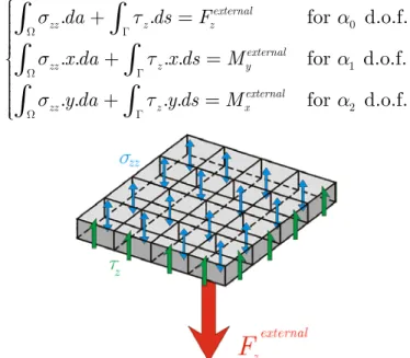
3D Coulomb friction law, with the transmission of the frictional effort perpendicular to the slice to the generalized plane strain state degrees of freedom, in order to take into account extraction force;
• the ferrostatic pressure element;
• the management of the large data collection on heat transfer coefficients in the water sprayed zones.
• The definition of heat transfer coefficients depending on the surface temperature of the strand and on the gap size in the mould (leading to a more stable convergence).
2D½ thermal-mechanical model of continuous casting using finite element method
13
• The determination of a simple way to degenerate parameters of the mechanical law and the coefficient of thermal linear expansion, so that the lack of compressibility of the liquid phase does not causes unwanted effects in this lagrangian slice approach.
• The application on the generalized plane strain state of an external force corresponding to the extraction force. This force can be either defined “externally” according to a curve supplied by the steel producer for the concerned caster and casting conditions, or it can be computed in a coupled way, according to the in-plane behaviour of the slice and the assumptions about friction of the rolls spinning around their axis or friction in the mould.
• The introduction of springs used to control slab bulging in secondary cooling, the determination of an analytical expression of the stiffness of these springs to obtain a more realistic bulging shape than the one obtained with classical 2D slice models and the calibration of this stiffness to fit maximum bulging obtained with a bulging model.
• The modification in the sequence of computation in the staggered time-stepping analysis: first thermal, then mechanical analysis (instead of the contrary as used in some applications in the team up till this model).
• Some post-processing developments to generate 3D views of the results obtained in the 2D½ slice mode, allowing better analysis of the temperatures, stresses and strains in the modelling of the slab bending/straightening.
• The adaptation of parts of the LAGAMINE code and numerical tools (as staggered analysis management and post-processing software) for PC and UNIX stations.
Finally, beside these numerical developments, an important part of the work concerned many meetings and discussions with industrial partners as well as with IRSID. The aims of these meetings were to present partial results and to examine some assumptions concerning the caster working (in the mould, distribution of extraction force…) and the slab bulging.
I
15
I
I
I
I
I
I
.
.
.
T
T
T
h
h
h
e
e
e
r
r
r
m
m
m
a
a
a
l
l
l
m
m
m
o
o
o
d
d
d
e
e
e
l
l
l
1. Solidification of alloys and steel
1.1. Crystalline structure
Most engineering materials are crystalline, that is to say that the atoms are arranged in a regular, structured and repeated manner. Each grain or crystallite is a kind of framework, characterized by the repetition of a unit cell. The length of the unit cell edges and the angles between crystallographic axes are referred as lattice parameters, which describe completely the geometry of the crystallite.
α γ β a b c
Figure 8: Geometry of a unit cell – the lattice parameters
Only seven different unit cells exist, they are represented in Table 1. They are also known as the seven crystal systems.
system edges angles unit cell
cubic a = b = c α = β = γ = 90° a a a tetragonal a = b ≠ c α = β = γ = 90° a a c orthorhombic a ≠ b ≠ c α = β = γ = 90° a b c
2D½ thermal-mechanical model of continuous casting using finite element method 16 rhombohedral a = b = c α = β = γ ≠ 90° α hexagonal a = b ≠ c α = β = 90° / γ = 120° a a c γ monoclinic a ≠ b ≠ c α = γ = 90° ≠ β a b c β triclinic a ≠ b ≠ c α ≠ β≠ γ ≠ 90° a b c
Table 1: Seven existing crystal systems
For a given crystal system, several dispositions of the atoms can be found to fill the 3D microstructure of the system. For example, with the cubic system, one can differentiate the simple cubic, the body-centred cubic (bcc) and the face-centred cubic (fcc) dispositions. Bravais classified 14 different ways to fill the 7 systems, also called the 14 crystal Bravais lattices:
simple cubic body-centred cubic face-centred cubic simple tetragonal body-centred tetragonal simple orthorhombic body-centred orthorhombic base-centred orthorhombic face-centred orthorhombic rhombohedral
hexagonal simple monoclinic base-centred monoclinic triclinic
Figure 9: The 14 crystal Bravais lattices
Majority of metals crystallize in one of the three high-symmetry lattices: body-centred cubic, face-body-centred cubic and hexagonal close packet, the latter being more
2D½ thermal-mechanical model of continuous casting using finite element method
17
complicated than the Bravais lattice with 3 additional atoms between parallel “horizontal” planes:
→
Figure 10: Hexagonal close packet lattice
Solid iron crystallises in two possible lattices: the body-centred cubic ferrite and face-centred cubic austenite.
Since the mass of the atoms constituting the crystal is known, it is possible to determine the mass density of the crystal. To do so, X-ray diffraction is used to determine spacing between adjacent planes (Bragg rule), then the ratio of mass to volume of one unit cell gives the mass density of the crystal.
1.2. Solid solutions
Up till now, only the perfectly repetitive structure of crystals has been considered, but it is not possible to avoid some contamination in practical materials. However, this contamination by impurities can be intentional, such as for metal alloys. As a result, many materials can be considered as solid solutions, which are homogeneous structures made of two or more components (distinct chemical substances).
There are two types of solid solutions:
• substitutional solid solutions: one component A (solute) dissolves in another one B (solvent), keeping the crystalline structure of the solvent B – for instance Ni dissolves in Cu crystalline structure;
• interstitial solid solutions: a smaller component A fit into free spaces of the crystalline structure of the larger component B – for instance C in ferrite crystal.
1.3. Phase diagrams
1.3.1. Pure materialsA phase is a chemically and structurally homogeneous portion of a microstructure. A single-phase microstructure can be polycrystalline, but each crystal grain only differs by its crystal orientation.
Any chemical substance can exist in different phases: gas, liquid and solid phases. Some components can present several solid phases, like pure iron, which presents two solid phases: ferrite (bcc) and austenite (fcc).
According to thermodynamics principles, the stable phase under some surroundings conditions (such as temperature and pressure) is the one presenting the lowest Gibbs free energy (at the equilibrium) in these conditions. The Figure 11 represents the
2D½ thermal-mechanical model of continuous casting using finite element method
18
evolution of Gibbs free energy for iron with respect to temperature (p = 1 atm) [COH94].
Figure 11: Gibbs free energy for iron with respect to temperature (p = 1 atm)
According to this figure:
• iron crystallise in bcc from room temperature up to 910°C - α-Fe (α-ferrite) • iron crystallise in fcc structure from 910°C up to 1394°C - γ-Fe (austenite) • iron crystallise in bcc structure from 1394°C up to 1538°C - δ-Fe (δ-ferrite) • iron is liquid above 1538 °C
When two curves intersect, for instance at 1538 °C, two phases are in equilibrium, so they can coexist. If the temperature is decreasing, only δ-ferrite phase is stable, so that the liquid phase solidifies into δ-ferrite phase. This is exactly the same at 1394°C when the crystalline structure of iron changes from δ-ferrite (bcc) to austenite (fcc) and at 910°C (back to bcc) when α-ferrite appears.
This can be illustrated by the Gibbs phase rule:
F =N − + (1) φ v
where F is the number of degrees of freedom or variance, N the number of
independent components, φ the number of phases in equilibrium and v the number of
state variables, in general 2 – temperature T and pressure p. The variance F
represents the number of state variables that can be changed without modification of the system phase.
For a pure metal (N = 1), the melting point corresponds to two simultaneous phases
(liquid and solid – φ = 2) and F = 1 – 2 + 2 = 1. That means that if one of the two
state variables is fixed (temperature or pressure), it exists only one value of the other one to maintain simultaneously the two phases. For example, if the pressure is fixed
(atmospheric pressure), it remains only one state variable (temperature – v = 1) and
F = 1 – 2 + 1 = 0, so that the temperature cannot be changed without changing the system configuration (liquid+solid phases). In other words, it exists only one temperature at which liquid and solid phases coexist. This is illustrated on Figure 12, which is the phase diagram of pure iron.
2D½ thermal-mechanical model of continuous casting using finite element method 19 temperature pressure α γ δ liquid gas solid 1 atm
Figure 12: Phase diagram of pure iron [SHA96]
A phase diagram is a graphical representation of the state variables associated with
microstructure. It divides the v-dimensions space (v being the number of state
variables) into different zones where only one phase exists. At the boundary (lines) between two zones, both phases are in equilibrium. The coordinates of the points
representing the boundaries correspond to the values of the states variables (T and p)
at which the equilibrium is possible.
When two lines get in touch, three phases can be in equilibrium: such a point is
called triple point. In such a case, φ = 3 and the Gibbs phase rule gives F = 1 – 3 +
2 = 0. That means that no state variable can be changed without modifying the system configuration, the triple point is unique. This is evident on the phase diagram (Figure 12): any modification of temperature or pressure implies the disappearing of at least one of the three phases.
1.3.2. Complete solid solutions
As already mentioned above, pure materials are exceptional and the presence of impurities increases the number of components in the system. For example, considering a solid solution of two components (binary system), the number of components becomes equal to 2. Another state variable appear in this case: the composition of the system.
Considering that pressure is fixed (generally in industrial applications, p = 1 atm),
two state variables are remaining: the Gibbs phase rule is thus F = 2 – φ + 1 = 3 –
φ. So that two phases (for example, solid and liquid phases) can be maintained
simultaneously in a range of temperature for a given composition as shown on Figure 13.
2D½ thermal-mechanical model of continuous casting using finite element method
20
Figure 13: Phase diagram for binary system (complete solid solution) [SHA96]
The upper boundary of the two-phase region is called liquidus, that is the line above which single liquid phase is present. The lower boundary is the solidus. Between solidus and liquidus, one can speak of semisolid state. Because of its consistency, semisolid state is also often called mushy state.
These two boundaries also represent the composition of both phases at a given
temperature. For instance, if the temperature is T1, the composition of liquid and
solid solution can be read on liquidus and solidus as shown on this figure:
Figure 14: Composition of the two phases during phase transformation [SHA96]
Such a system is a complete solid solution, which is characterized by the possibility to replace any amount of one component (up to 100%) by atoms of the other. To do so, the two components must be quite similar, as defined by Hume-Rothery rules: • less than 15% difference in atomic radii
2D½ thermal-mechanical model of continuous casting using finite element method
21
• similar electronegativities • same valence
If any rule is violated, only partial solubility (<100%) is possible. 1.3.3. Eutectic diagram without solid solution
Some components are so dissimilar that their solubility in each other is almost inexistent. That means that two different phases exist simultaneously at solid state: grains of pure A component beside grains of pure B can be observed.
At liquid state, both components are mixed, but when freezing, grains of either pure A, either pure B appear and grow, the other component remaining liquid.
However, for a given composition, both A and B components solidify at the same temperature, forming the so-called eutectic microstructure, characterized by fine alternative layers of A and B components.
The solidus is a horizontal line: the solidification always ends at the same temperature whatever is the composition, in particular for the eutectic composition, so that the solidus is also called eutectic temperature.
Figure 15: Binary eutectic phase showing no solid solution [SHA96]
1.3.4. Eutectic diagram with limited solid solution
For many binary systems, the two components present at least a partial solubility in each other. The phase diagram is thus quite similar to the previous one, except that B component can be solved in A component up to a limited concentration depending
on the temperature: this forms a phase α. In the same way, A can be solved in B
2D½ thermal-mechanical model of continuous casting using finite element method
22
Figure 16: Binary eutectic phase with limited solid solution [SHA96]
1.3.5. Eutectoid diagram
The eutectic transformation can be written:
cooling
eutectic
L → + (2) α β
Some binary systems presents the same kind of transformation, but a solid phase γ is
transformed into two other solid phases:
cooling
γ → + (3) α β
This eutectic-like transformation is called eutectoid. The corresponding temperature is the eutectoid temperature and the phase diagram is:
2D½ thermal-mechanical model of continuous casting using finite element method
23
1.3.6. Peritectic diagram
In the previous diagrams, pure components (A and B) have a distinct melting temperature. In some binary systems, the two components A and B can form a stable compound AB.
To simplify, consider that the solubility of AB intermediate compound is almost inexistent in both A and B. The peritectic transformation consists in a mixture of
solid solution and liquid (for instance L + B) transforming at constant temperature
into another solid solution for example (AB):
cooling heating
L+ ←B→AB (4)
This situation is illustrated by Figure 18.
Figure 18: Peritectic phase diagram [SHA96]
The components A and B are said to undergo congruent melting, since the liquid formed upon melting has the same composition as the solid from which it was formed. At the opposite, the compound AB is said to undergo incongruent melting, i.e. the liquid formed upon melting has not the same composition than AB. The peritectic term is used to describe the incongruent melting phenomenon.
1.3.7. Fe-Fe3C phase diagram
Steel is an alloy made of iron and carbon: Fe-C phase diagram should consequently be representative of equilibrium between both components of steel. However,
although graphite C is more stable than the compound Fe3C (cementite), the rate of
graphite precipitation is much slower than that of cementite. The result is that in common steels, the Fe3C phase is metastable, i.e. for all practical purposes it is stable with time and conforms to the Gibbs phase rule.
The Fe-Fe3C phase diagram is represented on Figure 19. Three of the phase diagrams
introduced above are present in Fe-Fe3C phase diagram:
• eutectic transformation (1148°C, 4.30wt%), eutectic composition being known as ledeburite;
• eutectoid transformation (727°C, 0.77wt%), eutectoid composition being known as pearlite;
2D½ thermal-mechanical model of continuous casting using finite element method
24
• peritectic transformation (1495°C, 0.18wt%), peritectic composition not having a specific name (simply austenite).
Note that ledeburite and pearlite are not phases. Only 4 phases exist in steel at any composition and temperature: these are bcc α-phase (ferrite), fcc γ-phase (austenite),
bcc δ-phase (δ-ferrite) and Fe3C compound (cementite). As already mentioned above,
eutectic and eutectoid compositions are made of fine alternative layers of two components: austenite and cementite for ledeburite, and ferrite and cementite for pearlite.
Figure 19: Fe-Fe3C phase diagram [SHA96]
The boundary between irons and steels is identified as a carbon content of 2.11wt%, which corresponds to the carbon solubility limit in the austenite γ-phase. Amongst
2D½ thermal-mechanical model of continuous casting using finite element method
25
the steels, a common distinction between hyper- and hypo-eutectoid corresponds precisely to carbon content higher or lower than 0.77wt%.
Another distinction is made between low carbon steel (carbon content < 0.18wt%) and carbon steel (> 0.18wt%), i.e. below or over the carbon content in the peritectic
composition (see detail of Fe-Fe3C phase diagram in peritectic region on Figure 20).
The difference between low carbon and carbon steels is the presence of δ-ferrite phase after the complete solidification and the δ→γ phase transformation at solid state, which affects some material properties such as mass density and thermal expansion.
Figure 20: Fe-Fe3C phase diagram in the peritectic region
1.4. The lever rule
This rule is used to determine in a two-phase region the amount of each phase. The relative amounts of the two phases can be easily determined from a mass balance. Consider the simple case of the phase diagram of a complete solid solution. Initially,
the composition is assumed to be liquid. It contains x0% of B, thus 100%-x0% of A
component. While the temperature is decreasing down to liquidus, the composition remains the same. From the liquidus, solid solution appears and when the temperature reaches the solidus, only solid solution remains.
In the two-phase region, the sum of mass percentage of both phases (solid solution %SS and liquid %L) is equal to 100%:
2D½ thermal-mechanical model of continuous casting using finite element method
26
In other respects, the total amount of B component is constant and equal to x0. Since
the amounts of B in the solid solution (xSS) and the liquid (xL) are given by the
solidus and liquidus curves, their sum must be equal to:
0 .% .% L SS x L+x SS =x (6) Introducing (5) in relation (6):
(
)
0 . 100% % .% L SS x − SS +x SS =x (7) or 0 % L 100% 100% L SS x x b SS x x a b − = = − + (8) and 0 % 100% % SS 100% 100% L SS x x a L SS x x a b − = − = = − + (9)where a and b are the length of the segment represented on the following figure:
a b xL x0 xSS T1 L SS L+SS A B
Figure 21: Lever rule
This rule is known as the lever rule (because of a mechanical analogy with a lever balanced on fulcrum).
Relations (8) and (9) are defining the fraction of each component. Instead of percentage, fractions are generally expressed in term of natural value (no unit):
% liquid fraction = 100% % solid fraction = 100% L s L a f a b SS b f a b = = + = = + (10)
They are complementary, their sum being equal to unity so that: 1
L s
2D½ thermal-mechanical model of continuous casting using finite element method
27
1.5. Steel compostion during solidification: examples
The composition of two phases during phase transformation – Figure 14 – and the lever rule introduced above – relations (10) – allow studying the complete evolution of any alloy during solidification.
Consider for example steel at 3 different compositions in the peritectic region: • a 0.05wt% low carbon steel
• a 0.15wt% low carbon steel • a 0.42wt% carbon steel
The solidification of each one is be characterized by the apparition of different phases at different temperatures:
Figure 22: Solidification of 3 different compositions of steel
a. 0.05wt% low carbon steel Characteristic temperatures are:
• liquidus: 1538 (1495 1538)0.05 1534°C 0.51 L T = + − = • solidus: 1538 (1495 1538)0.05 1516.5°C 0.10 S T = + − = • δ→γ beginning: 1394 (1495 1394)0.05 1444.5°C 0.10 Tδ = + − =
2D½ thermal-mechanical model of continuous casting using finite element method
28
• δ→γ ending: 1394 (1495 1394)0.05 1422°C
0.18
Tγ = + − =
The following table summarize for each temperature range the carbon content in each phase (CL, Cδ and Cγ) and the fraction of each phase (fL, fδ and fγ).
L T <T TS <T <TL Tδ <T <TS Tγ <T <Tδ T <Tγ CL 0.05 % 1538 0.51% 1538 1495 T − − - - - L-phase fL 1 ( ) ( ) ( ) 0.05% L C T C T C T δ δ − − 0 0 0 Cδ - 1538 0.10% 1538 1495 T − − 0.05 % 1394 0.10% 1495 1394 T − − - δ-phase fδ 0 ( ) ( ) ( ) 0.05% L L C T C T C Tδ − − 1 ( ) ( ) ( ) 0.05% C T C T C T γ δ γ − − 0 Cγ - - - 1394 0.18% 1493 1394 T − − 0.05 % γ-phase fγ 0 0 0 ( ) ( ) ( ) 0.05% C T C T C T δ δ γ − − 1 For instance, at 1520°C, the material is made of liquid and δ-phase:
• carbon content in liquid is equal to 1538 15200.51% 0.213%
1538 1495
L
C = − =
−
• carbon content in δ-phase is equal to 1538 15200.10% 0.042%
1538 1495 Cδ = − = − • liquid fraction is 0.05% 0.042% 0.047 0.213% 0.042% L f = − = − • δ-phase fraction is 0.213% 0.05% 0.953 0.213% 0.042% fδ = − = −
One can easily verify that the total carbon content at 1520°C is still: 0.213wt% 0.047 + 0.042wt% 0.953 = 0.05wt%
The Figure 23 shows the evolution with respect to temperature of liquid, δ-ferrite and γ-austenite phases and their carbon content in this 0.05wt%C low carbon steel.
2D½ thermal-mechanical model of continuous casting using finite element method
29
0.05%C Low carbon steel
0.0 0.1 0.2 0.3 0.4 0.5 0.6 0.7 0.8 0.9 1.0 1400 1410 1420 1430 1440 1450 1460 1470 1480 1490 1500 1510 1520 1530 1540 1550 Temperature (°C) Fr ac ti on
liquid fraction delta fraction gamma fraction
0.05%C Low carbon steel
1400 1410 1420 1430 1440 1450 1460 1470 1480 1490 1500 1510 1520 1530 1540 1550 Temperature (°C) 0.00 0.05 0.10 0.15 0.20 0.25 0.30 %C %C in liquid phase %C in delta phase %C in gamma phase
Figure 23: Fraction of liquid, δ-ferrite and γ-austenite phases and their carbon content in a 0.05wt%C low carbon steel with respect to temperature
b. 0.15wt% low carbon steel Characteristic temperatures are:
• liquidus: 1538 (1495 1538)0.15 1525°C
0.51 L
T = + − =
• solidus: T =S 1495°C and δ→γ beginning: Tδ =1495°C
• δ→γ ending: 1394 (1495 1394)0.15 1478°C
0.18
Tγ = + − =
Note that the solidus corresponds to the apparition of both δ- and γ-phases (peritectic temperature). Hence the following table:
L T <T TS <T <TL T =Tδ =TS Tγ <T <Tδ T <Tγ CL 0.15 % 1538 0.51% 1538 1495 T − − - - - L-phase fL 1 ( ) ( ) ( ) 0.15% L C T C T C T δ δ − − 0.122 → 0 0 0 Cδ - 1538 0.10% 1538 1495 T − − 0.10% 1394 0.10% 1495 1394 T − − - δ-phase fδ 0 ( ) ( ) ( ) 0.15% L L C T C T C Tδ − − 0.878 → 0.375 ( ) ( ) ( ) 0.15% C T C T C T γ δ γ − − 0 Cγ - - 0.18% 1394 0.18% 1493 1394 T − − 0.15 % γ-phase fγ 0 0 0 → 0.625 ( ) ( ) ( ) 0.15% C T C T C T δ δ γ − − 1
2D½ thermal-mechanical model of continuous casting using finite element method
30
The Figure 24 shows the evolution with respect to temperature of liquid, δ-ferrite and γ-austenite phases and their carbon content in this 0.15wt%C low carbon steel.
0.15%C Low carbon steel
0.0 0.1 0.2 0.3 0.4 0.5 0.6 0.7 0.8 0.9 1.0 1400 1410 1420 1430 1440 1450 1460 1470 1480 1490 1500 1510 1520 1530 1540 1550 Temperature (°C) Fr ac ti on
liquid fraction delta fraction gamma fraction
0.15%C Low carbon steel
1400 1410 1420 1430 1440 1450 1460 1470 1480 1490 1500 1510 1520 1530 1540 1550 Temperature (°C) 0.00 0.05 0.10 0.15 0.20 0.25 0.30 0.35 0.40 0.45 0.50 0.55 0.60 %C %C in liquid phase %C in delta phase %C in gamma phase
Figure 24: Fraction of liquid, δ-ferrite and γ-austenite phases and their carbon content in a 0.15wt%C low carbon steel with respect to temperature
c. 0.42wt% carbon steel
Characteristic temperatures are:
• liquidus: 1538 (1495 1538)0.42 1502.5°C 0.51 L T = + − = • L+δ→ L+γ transformation: Tδ γ→ =1495°C • solidus: 1495 (1148 1495)0.42 0.18 1452°C 2.11 0.18 S T = + − − = − L T <T Tδ γ→ <T <TL T =Tδ γ→ TS <T <Tδ γ→ T <TS CL 0.42 % 1538 0.51% 1538 1495 T − − 0.51% 1495 0.51% 3.79% 1495 1148 T − + − - L-phase fL 1 ( ) ( ) ( ) 0.42% L C T C T C T δ δ − − 0.780 → 0.723 ( ) ( ) ( ) 0.42% L C T C T C T γ γ − − 0 Cδ - 1538 0.10% 1538 1495 T − − 0.10% - - δ-phase fδ 0 ( ) ( ) ( ) 0.42% L L C T C T C Tδ − − 0.220 → 0 0 0 Cγ - - 0.18% 14950.18% 1.93% 1495 1148 T − + − 0.42 % γ-phase fγ 0 0 0 → 0.273 ( ) ( ) ( ) 0.42% L L C T C T C Tγ − − 1
![Figure 28: Variation of mean thermal linear expansion coefficient of 0.05wt%C, 0.15wt%C and 0.42wt%C steels [CHA93]](https://thumb-eu.123doks.com/thumbv2/123doknet/5440392.127879/49.892.259.677.132.414/figure-variation-mean-thermal-linear-expansion-coefficient-steels.webp)