An Empirical Study of Credit Shock Transmission in a Small Open Economy

Texte intégral

(1)2012s-16. An Empirical Study of Credit Shock Transmission in a Small Open Economy Nathan Bedock, Dalibor Stevanović. Série Scientifique Scientific Series. Montréal Juin 2012. © 2012 Nathan Bedock, Dalibor Stevanović. Tous droits réservés. All rights reserved. Reproduction partielle permise avec citation du document source, incluant la notice ©. Short sections may be quoted without explicit permission, if full credit, including © notice, is given to the source..

(2) CIRANO Le CIRANO est un organisme sans but lucratif constitué en vertu de la Loi des compagnies du Québec. Le financement de son infrastructure et de ses activités de recherche provient des cotisations de ses organisations-membres, d’une subvention d’infrastructure du Ministère du Développement économique et régional et de la Recherche, de même que des subventions et mandats obtenus par ses équipes de recherche. CIRANO is a private non-profit organization incorporated under the Québec Companies Act. Its infrastructure and research activities are funded through fees paid by member organizations, an infrastructure grant from the Ministère du Développement économique et régional et de la Recherche, and grants and research mandates obtained by its research teams. Les partenaires du CIRANO Partenaire majeur Ministère du Développement économique, de l’Innovation et de l’Exportation Partenaires corporatifs Autorité des marchés financiers Banque de développement du Canada Banque du Canada Banque Laurentienne du Canada Banque Nationale du Canada Banque Royale du Canada Banque Scotia Bell Canada BMO Groupe financier Caisse de dépôt et placement du Québec Fédération des caisses Desjardins du Québec Financière Sun Life, Québec Gaz Métro Hydro-Québec Industrie Canada Investissements PSP Ministère des Finances du Québec Power Corporation du Canada Rio Tinto Alcan State Street Global Advisors Transat A.T. Ville de Montréal Partenaires universitaires École Polytechnique de Montréal HEC Montréal McGill University Université Concordia Université de Montréal Université de Sherbrooke Université du Québec Université du Québec à Montréal Université Laval Le CIRANO collabore avec de nombreux centres et chaires de recherche universitaires dont on peut consulter la liste sur son site web. Les cahiers de la série scientifique (CS) visent à rendre accessibles des résultats de recherche effectuée au CIRANO afin de susciter échanges et commentaires. Ces cahiers sont écrits dans le style des publications scientifiques. Les idées et les opinions émises sont sous l’unique responsabilité des auteurs et ne représentent pas nécessairement les positions du CIRANO ou de ses partenaires. This paper presents research carried out at CIRANO and aims at encouraging discussion and comment. The observations and viewpoints expressed are the sole responsibility of the authors. They do not necessarily represent positions of CIRANO or its partners.. ISSN 1198-8177. Partenaire financier.

(3) An Empirical Study of Credit Shock Transmission in a Small Open Economy Nathan Bedock*, Dalibor Stevanović †. Résumé / Abstract In this paper we identify and measure the effects of credit shocks in a small open economy. To incorporate information from a large number of economic and financial indicators we use the structural factor-augmented VARMA model. In the theoretical framework of the financial accelerator, we approximate the external finance premium with credit spreads. We find that an adverse global credit shock generates a significant and persistent economic slowdown in Canada; the Canadian external finance premium rises immediately while interest rates and credit measures decline. Variance decomposition reveals that the credit shock has an important effect on real activity measures, including price and leading indicators, and credit spreads. On the other hand, an unexpected increase in the Canadian external finance premium shows no significant effect in Canada, suggesting that the effects of credit shocks in Canada are essentially caused by the unexpected changes in foreign credit market conditions. Given the identification procedure our structural factors have an economic interpretation. Mots clés/Keywords : Credit shock, structural factor analysis, factoraugmented VARMA. Codes JEL: E32, E44, C32. *. HEC Montréal, email: Nathan.bedock@hec.ca CIRANO et Université du Québec à Montréal, Département des sciences économiques. Mailing address: Université du Québec à Montréal, Département des sciences économiques, 315, rue Ste-Catherine Est, Montréal, Québec, H2X 3X2, e-mail: dstevanovic.econ@gmail.com (corresponding author). This project was completed while I was Visiting Scholar at the University of Pennsylvania. I wish to thank the Department of Economics at UPenn for its hospitality. †.

(4) Contents 1 Introduction. 1. 2 Theoretical framework. 3. 3 Econometric framework in data-rich environment. 4. 3.1. Factor-augmented VARMA model . . . . . . . . . . . . . . . . . . . . . . . . . . . . . . . . .. 5. 3.2. Estimation . . . . . . . . . . . . . . . . . . . . . . . . . . . . . . . . . . . . . . . . . . . . . .. 7. 3.3. Identification of structural shocks . . . . . . . . . . . . . . . . . . . . . . . . . . . . . . . . . .. 8. 4 Data. 9. 5 Results. 10. 5.1. Global credit shock . . . . . . . . . . . . . . . . . . . . . . . . . . . . . . . . . . . . . . . . . .. 10. 5.2. Canadian credit shock . . . . . . . . . . . . . . . . . . . . . . . . . . . . . . . . . . . . . . . .. 12. 5.3. Further robustness analysis . . . . . . . . . . . . . . . . . . . . . . . . . . . . . . . . . . . . .. 13. 5.4. Interpretation of factors . . . . . . . . . . . . . . . . . . . . . . . . . . . . . . . . . . . . . . .. 15. 6 Conclusion. 15. ii.

(5) 1. Introduction. The current economic downturn suggests that there is information in the financial sector that has not been integrated into our understanding of macroeconomics. Studies by Stock and Watson (1989,2003), Estrella and Hadrouvelis (1991), Gertler and Lown (1999), Diebold et al. (2006), Mueller (2007), and Gilchrist, Yankov, and Zakrajsek (2009) have shown that there is predictive content in financial series. The results in Forni et al. (2003) show that financial variables are important when forecasting inflation rates but do not help in predicting industrial production, which is also confirmed in Espinoza et al. (2009). Moreover, the nonneoclassical monetary policy transmission mechanisms which are related to credit markets are theoretically and empirically under-documented. Here, we propose to empirically measure the impact of credit shocks in Canada within this theoretical framework. Due to the complexity of credit markets, we doubt that their informational content can be synthesized in as few variables as a vector autoregressive (VAR) model allows us. In order to incorporate information from a large number of economic and financial indicators, we will use the structural factor analysis approach proposed by Bernanke et al. (2005), Marcellino and Kapetainous (2005), and Stock and Watson (2005), among others. In particular, we will use a factor-augmented VARMA (FAVARMA) model proposed by Dufour and Stevanovic (2010). This is a theoretically coherent model with an approach that combines two dimension reduction techniques: factor analysis and VARMA modeling. The identification of structural shocks is achieved by imposing a recursive structure on the impact matrix of the structural MA representation of observable variables. Similar studies have been made for the US economy by Boivin, Giannoni, and Stevanovic (2009b) (BGS hereafter) and Gilchrist, Yankov, and Zakrajsek (2009). Both studies find that credit shocks have wide effects on the economy that are consistent with a significant economic slowdown. Pesaran et al. (2006) use the global VAR model to link the firm-specific changes in the credit portfolio to macroeconomic business cycles. Safei and Cameron (2003) and Atta-Mensah and Dib (2008) have studied the dynamics of the Canadian credit market, the former employing a structural VAR approach, the latter using a general equilibrium approach. The conclusions drawn by Safei and Cameron (2003) show a lack of robustness, suggesting that there is information missing in their structural VAR models. The present exercise tries to correct this problem by using a large data set. The results of Atta-Mensah and Dib (2008) are more coherent with the dynamic stochastic general equilibrium (DSGE) literature describing credit market models, except that they consider Canada as a closed economy. Our methodology will allow us to include more information about the global financial market and to simulate shocks from outside of Canada, which will be important in our following 1.

(6) discussion. Our results show that an unexpected increase in the external finance premium on global financial markets, approximated by the US credit spread, generates a significant and persistent economic slowdown in Canada. Canadian credit spreads rise immediately, while interest rates and credit measures decline. Contrary to existing work on the Canadian economy, we find that price indexes fall persistently1 . Since we do not impose timing restrictions on forward-looking variables, these leading indicators respond negatively on impact, as expected. This gives a more realistic picture of the effect of credit shocks on the economy and provides information about the transmission mechanism of these shocks. According to R2 results, the common component captures an important dimension of the business cycle movements. From the variance decomposition analysis, we observe that the credit shock has an important effect on several real activity measures including price indicators, leading indicators, and credit spreads. Another piece of important empirical evidence concerns the identification of national financial shocks. Previous studies have treated Canada as a closed economy when identifying a credit shock and have found some real effects. Our results suggest that there is no significant effect of domestic shocks in Canada. Indeed, the effects of credit shocks in Canada are essentially caused by unexpected changes in foreign credit market conditions. In robustness analysis, we compare our benchmark results after the US credit shock to two other factor representations with different identification schemes. The dynamic responses for many variables are quite similar and confirm our previous findings. Finally, a by-product of our identification approach is a rotation matrix that can be used to recover the structural factors. These rotation matrices still have the same informational content, but their interpretation, in terms of the correlation structure, can change. Indeed, we find that the rotated principal components do have an economic interpretation. In the rest of the paper, we first present the theoretical framework in which credit shocks can occur. Then, we present our econometric framework in a data-rich environment and discuss the estimation and identification issues. The main results are presented in Section 5, followed by a conclusion. The Appendix contains some additional results, an explanation of the bootstrap procedure, and the data description. 1 A FAVAR analysis includes more information than a VAR and less structure than a DSGE. Other FAVAR studies find a fall in price indexes where VAR and DSGE studies concerning the Canadian economy do not.. 2.

(7) 2. Theoretical framework. In this section we briefly discuss how the financial and economic sides are connected and through which channel(s) shocks on the credit market could affect economic activity. Financial frictions are crucial when linking credit market conditions to economic activity. We see this from the fact that in a framework of incomplete information, the Modigliani-Miller theorem does not apply. This means that a firm’s value is determined by its capital structure. After aggregation and if credit markets determine capital structure in the economy, we should observe informational frictions characterizing the firm’s value. Frictions can arise from both supply and demand. On the supply side, usually interpreted as the bank lending channel, Bernanke (1993) observes that banks and other financial intermediaries are able to fund projects which are complex to evaluate, using funds from investors that have only partial information about these projects. If banks resolve asymmetric information problems in the credit market, they can be considered credit creators and their health becomes an important macroeconomic parameter. However, because of the democratization of credit in the 1980s, informational frictions on the supply side seem to be less present. Dynan et al. (2006) provide empirical evidence that households’ expenses are less sensitive to their income, encouraging us to look for other kinds of frictions. On the demand side, which links to the balance sheet channel, Bernanke et al. (1999) (BGG hereafter) introduce the idea of a financial accelerator working through the interaction of two measures. The first is the external finance premium, defined as the difference between the external cost of capital and the internal opportunity cost of capital. The second is the net worth of potential borrowers, which is used to measure the collateral that firms are able to offer to obtain credit. The idea of the financial accelerator is that there is an inverse relationship between these two measures. If the net worth of a firm falls, the collateral value that it will be able to present to banks will also fall. Similarly, the firm’s contribution to capital will also decline. In consequence, the bank will possess relatively more parts of the firm, creating an agency cost to solve the divergence between the two parts. This agency cost will raise the external finance premium, i.e. the firm’s capital cost. Thus, the financial accelerator mechanism works as follows: a fall in net worth (due to a financial crisis, for example) raises the acquisition capital cost, pushing firms to invest a sub-optimal quantity of capital and creating a persistent effect from the original crisis. Building on BGG, Gilchrist, Ortiz, and Zakrajsek (2009) aim to quantify the role of financial frictions in generating business cycle fluctuations. They augment a standard DSGE model with the financial accelerator mechanism which links the conditions in the credit market to the real economy through the external finance 3.

(8) premium. Two financial shocks are introduced: a financial disturbance shock, which affects the external finance premium, and a net worth shock affecting the balance sheet of a firm. The first shock is presented as a credit supply shock, which Christiano et al. (2009) interpret as an increase in the agency costs due to a higher variance of idiosyncratic shocks affecting the firm’s profitability. The second shock can be viewed as a credit demand shock. Its effect will depend on the degree of frictions in the financial market. After estimating the structural model, the authors find that both financial shocks cause an increase in the external finance premium, which, through the financial accelerator, implies a slowdown in economic activity. Finally, Bloom (2009) provides a framework to analyze the impact of uncertainty shocks. He finds that increased volatility generates short, but sharp, recessions and recoveries.. 3. Econometric framework in data-rich environment. As information technology improves, the availability of economic and financial time series grows in terms of both time and cross-section size. However, a large amount of information can lead to the curse of dimensionality when standard time series tools are used. Since most of these series are highly correlated, at least within some categories, their co-variability pattern and informational content can be approximated by a smaller number of variables. A popular way to address this issue is to use factor analysis. The structural factor model approach will here be used to identify a structural shock and its effects on the economy. Previous studies have used standard VAR techniques with recursive identification schemes to identify credit shocks. However, as Bernanke et al. (2005) pointed out, the small-scale VAR model presents three issues. First, due to the small amount of information in the model, relative to the information set potentially observed by agents, VAR suffers from an omitted variable problem, which can alter the impulse response analysis. The second problem in a small-scale VAR model is that the choice of a specific data series to represent a general economic concept is arbitrary. Moreover, measurement errors, aggregations, and revisions present additional problems when linking theoretical concepts to specific data series. Even if the previous problems do not occur, we can only produce impulse responses for the variables included in the VAR. Finally, Forni et al. (2009) argues that while non-fundamentalness is generic in a small-scale models, it cannot arise in a large dimensional dynamic factor models2 . This is of primary importance, since the objective is to identify a relatively new structural shock in empirical macroeconomics. 2 If the shocks in the VAR model are fundamental, then the dynamic effects implied by the moving average representation can have a meaningful interpretation, i.e. the structural shocks can be recovered from current and past values of observable series.. 4.

(9) One way to address all of these issues is to take advantage of the information contained in large panel data sets using dynamic factor analysis and the factor-augmented VAR (FAVAR) model in particular. The importance of large data sets and factor analysis is well documented in both forecasting macroeconomic aggregates and structural analysis. Boivin et al. (2009a) have recently shown that incorporating information through a small number of factors corrects for several empirical puzzles when estimating the effect of monetary policy shocks in a small open economy. However, Dufour and Stevanovic (2010) argue that in general, multivariate series and their associated factors do not both follow a finite order VAR process. Hence, they propose a FAVARMA framework that combines two parsimonious methods to represent the dynamic interactions between a large number of time series: factor analysis and VARMA modeling.. 3.1. Factor-augmented VARMA model. Using the notation from Dufour and Stevanovic (2010), the dynamic factor model (DFM) where factors have a finite order VARMA(pf ,qf ) representation can be written as. Xit. ˜ i (L)ft + uit , = λ. uit. = δi (L)ui,t−1 + νit. (2). =. (3). ft. i = 1, . . . , N,. t = 1, . . . , T. Γ(L)ft−1 + Θ(L)ηt ,. (1). ˜ i (L) is a lag polynomial, δi (L) is a px,i -degree lag polynomial, Γ(L) = [Γ1 L + . . . + Γp Lpf ], where λ f Θ(L) = [I − Θ1 L − . . . − Θqf Lqf ], and νit is an N -dimensional white noise uncorrelated with q-dimensional white noise process ηt . The equation (1) relates observable variable Xit to q (latent) factors, ft , and to its ˜ i (L)ft is called the common component. We also allow for some idiosyncratic component, uit . The element λ limited cross-section correlations among the idiosyncratic components3 .. Subtracting δi (L)uit−1 from both sides of (1) gives the DFM with serially uncorrelated idiosyncratic errors:. Xit = λi (L)ft + δi (L)Xit−1 + νit ,. (4). 3 So that there exists a small number of largest eigenvalues of the covariance matrix of common components that diverge when the number of series tends to infinity, while the remaining eigenvalues as well as the eigenvalues of the covariance matrix of specific components are bounded. See Bai and Ng (2008) for an overview of the modern factor analysis literature, and the distinction between exact and approximate factor models.. 5.

(10) ˜ i (L). where λi (L) = (1 − δi (L)L)λ Then, we can rewrite the DFM in the following form:. Xt ft. = λ(L)ft + D(L)Xt−1 + νt. (5). =. (6). Γ(L)ft−1 + Θ(L)ηt ,. where.   λ1 (L)  .. λ (L) =  .   λn (L). . . .   δ1 (L) · · ·   .. ..  , D (L) =  . .     0 ···. .   ν1t    , νt =  ...     νnt δn (L) 0 .. ..    .  . ˜ To obtain the static version of the previous factor model suppose that λ(L) has finite degree p-1, and let Ft = [ft0. 0 0 ft−1 . . . ft−p+1 ]0 . Let the dimension of Ft be K, where q ≤ K ≤ qp. Then,. Xt. =. ΛFt + ut. (7). ut. =. D(L)ut−1 + νt. (8). Ft. =. Φ(L)Ft−1 + GΘ(L)ηt. (9). ˜ i (L), Φ(L) contains coefficients of Γ(L) where Λ is a N × K matrix whose ith row consists of coefficients of λ and zeros, and G is a K × q matrix (consisting of 1’s and 0’s) that loads (structural) shocks ηt to static factors. Note that if Θ(L) = I, we obtain the factor-augmented VAR (FAVAR) model. Finally, since the VARMA models are not identified in general, we will impose the diagonal moving average representation that is presented in following definition.. Definition 1 (Diagonal MA equation form) Suppose N -dimensional stochastic process Xt has the following VARMA representation: Φ(L)Xt = Θ(L)ut 6.

(11) This VARMA representation is said to be in diagonal MA equation form if Θ(L) = diag[θii (L)] = IN − Θ1 L − · · · − Θq Lq where θii (L) = 1 − θii,1 L − · · · − θii,qi Lqi , θii,qi 6= 0, and q = max1≤i≤N (qi ).. From the point of view of practitioners, this form is very appealing since adding lags of uit to the ith equation is a natural extension of the VAR model. It also has the advantage of giving a simple structure to the MA polynomials, the part which complicates the estimation.. 3.2. Estimation. We will work with the static version (7-9). Also, we assume the same number of dynamic and static factors, G = I, and no autocorrelations in the idiosyncratic component, D(L) = 0, which gives the following simplified model:. Xt. =. ΛFt + νt. (10). Ft. =. Φ(L)Ft−1 + Θ(L)ηt ,. (11). To estimate this model, we use the two-step Principal Component Analysis (PCA) estimation method (see Stock and Watson, 2002; and Bai and Ng, 2006; for theoretical results concerning the PCA estimator). In the first step, Fˆt are computed as K principal components of Xt . In the second step, we estimate the VARMA representation (11) using Fˆt . The standard estimation methods for VARMA models are maximum likelihood and non-linear least squares. Unfortunately, these methods require non-linear optimization, which may not be feasible when the number of parameters is relatively large. In this paper, we will use the GLS method proposed in Dufour and Pelletier (2008). Since the unobserved factors are estimated and then included as regressors in the FAVARMA model, the two-step approach suffers from the “generated regressors”problem. To get an accurate statistical inference on the impulse response functions that accounts for uncertainty associated with factors estimation, we use a bootstrap procedure suggested by Yamamoto (2009) and implemented in Dufour and Stevanovic (2010). The details of the bootstrap procedure are presented in the Appendix.. 7.

(12) 3.3. Identification of structural shocks. To identify the structural shocks, we adapt the contemporaneous timing restrictions procedure proposed in Stock and Watson (2005) to the FAVARMA framework. After inverting the VARMA process of factors in (11), assuming stationarity, and plugging it into (10), we obtain the MA representation of Xt :. Xt. =. Λ[I − Φ(L)L]−1 Θ(L)ηt + ut. = B(L)ηt + ut .. (12). We assume that the number of static factors, K, is equal to the number of dynamic factors and that residuals in (11) are linear combinations of structural shocks εt. εt = Hηt ,. (13). where H is a nonsingular square matrix and E[εt ε0t ] = I. Replacing (13) in (12) gives the structural MA form of Xt :. Xt. =. Λ[I − Φ(L)L]−1 Θ(L)H −1 εt + ut. = B ? (L)εt + ut .. (14). To achieve the identification of shocks in εt , the contemporaneous timing restrictions are imposed on the impact matrix in (14)         ? ? B0 ≡ B (0) =        . x. x. ··· .. .. x. x. ... .. 0. x .. .. x .. .. ··· .. .. x .. .. x. x. ···. x. x. 0. 0 0.         .       . ? Let B0:K = B0:K H −1 be a K × K lower triangular matrix, where B0:K contains the first K rows of B0 .. 8.

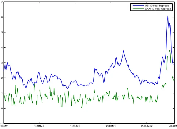
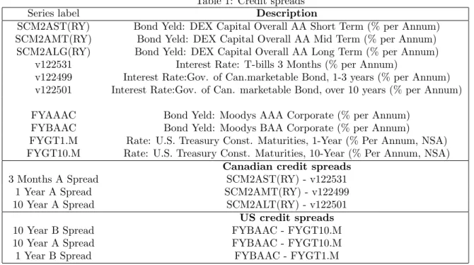
(13) Then, H is obtained as 0 H = [Chol(B0:K Σe B0:K )]−1 ΛK ,. (15). where Ση is the covariance matrix of ηt and ΛK is a K × K matrix of the first K rows of Λ. To estimate H, we just plug in the estimates of B0:K , Σe and ΛK . Hence, the impulse responses to any shock in εt are obtained using (14). This identification procedure is similar to the standard recursive identification in VARMA models. To just identify the K structural shocks, we need to impose K(K − 1)/2 restrictions. Imposing them in a recursive way makes estimation of the rotation matrix H easy. Also, it should be noted that the number of static factors must be equal to the number of series used in the recursive identification. Moreover, contrary to other identification strategies in the FAVAR literature, we do not need to impose any observed factor or rely on the interpretation of a particular latent factor. Remark that we follow the strategy to impose the minimum number of restriction by choosing the impact response of only K variables. Since there are many series in Xt , another possibility is to over-identify the model by imposing zero restrictions on more than K series. In that case, B ? would be block lower triangular. While, if all these additional restrictions are satisfied, this would produce more efficient results, our approach is more robust, and we believe more appropriate in this type of structural analysis.. 4. Data. The majority of our data comes from Dufour and Stevanovic (2010). It contains 332 monthly StatCan series that synthesize real and financial Canadian activity. Also included are variables describing a small open economy: exchange rates and global financial information. The time span is from January 1986 to November 2009. Credit spreads measuring credit market conditions are also included as additional series. A credit spread is defined as the difference between the actuarial rate of a firm bond and the actuarial rate of a risk-free product (typically a treasury bond). We were built American credit spreads using Moody’s bond index as described in BGS. Canadian credit spreads were built using a Canadian Dex bond index rated AA. Table 1 synthesizes information about the credit spread for Canada and the US. Because our results are very similar from one spread to another, we have selected a Canadian 10-Year A spread and an American 10-Year B spread. The two series are plotted in Figure 1.. 9.

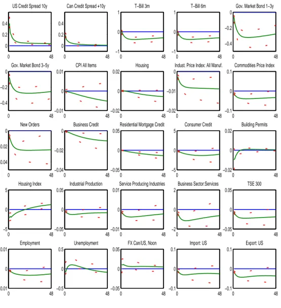
(14) 5. Results. The goal of this paper is to measure the dynamic effects of credit shocks on economic activity in Canada. Since we are looking at a small open economy it is important to control for any global influence on financial markets when identifying the credit shock effects. In previous studies, authors have considered Canada to be a closed economy, but our empirical evidence suggests this could be misleading. Indeed, our results show that the effect of a credit shock is essentially driven by global financial conditions and by US credit markets in particular. Given the fact that the US represents around 80% of foreign trade in Canada, we approximate the world financial conditions with the US proxies. Hence, we use the US 10-year credit spread (USspread10y) in the recursive identification scheme. On the other hand, we take the Canadian 10-year credit spread (CANspread10y) as a proxy to identify the national credit shock. In all specifications the lag order tests suggest a VARMA(2,1) process for the extracted factors.. 5.1. Global credit shock. ? is lower trianTo identify the global credit shock, we impose the following recursive scheme such that B0:K. gular:. [U Sspread10y,. CP I,. U R,. M S,. R,. F X],. where CP I is the Consumer Price Index: all items, U R is the Unemployment Rate, M S is the Money Base, R is the 3-month Treasury Bill and F X stands for the Can/US Exchange Rate. The credit shock is the first element in εt . This identification scheme implies that Canadian CPI, UR, MS, R and FX can respond immediately to a credit shock in the US. In other words, the contemporaneous response to a credit shock of all 349 variables is completely unrestricted. The impulse responses for some variables of interest are presented in Figure 2. A one-standard deviation credit shock immediately raises the US credit spread by 0.4 basic points, while the effect on the Canadian spread is two times smaller. This unexpected increase in the global external finance premium generates a significant and persistent economic downturn. We see that economic activity indicators such as production, employment, hours, prices and wages decline significantly. Production measures in particular go down for more than a year. Employment is also negatively affected, especially in the construction sector4 . All 4 We. have looked at all of the employment series responses and find that the magnitude responses vary across sectors. For. 10.

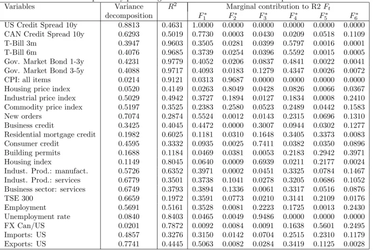
(15) consumer price indexes show approximately the same pattern of a gradual and highly persistent slowdown, but most are non-significant. On the other hand, the industrial and commodities price indexes respond in a statistically significant way and stay below their steady-state value. This result is different from what Atta-Mensah and Dib (2008), and Safaei and Cameron (2003) report, where prices rise in response to a credit shock5 . The effects on financial markets are even more striking. Treasury bills and government market bonds respond negatively and the effect is significant and persistent. Business and consumer credit measures decline. Leading indicators such as new orders, building permits and housing also start responding negatively on impact. Our econometric framework allows the possibility of measuring the effects of structural shocks across different economic activity sectors, as well as across geographical regions. This is important in the case of Canada because of its huge territory and small overall population density. Thus, it is interesting to see how the credit shocks propagate across different regions. The results are presented in Figure 6 in the Appendix. It seems that in general, the Atlantic provinces demonstrate the most inconsistent behavior with respect to the rest of Canada. The variance decomposition results are presented in Table 2. The second column reports the contribution of the credit shock to the variance of the forecast error at a 48-month horizon. According to these results, and contrary to the literature on monetary policy shocks identified in structural VAR framework, the global credit shock has an important effect on several variables: credit spreads, interest rates, industrial price indexes, credit measures, production and employment. This surprising evidence of the importance of credit shocks is also documented in BGS. Finally, since we are using a factor model, the natural question is how well the extracted factors explain the variability in the observable series. Looking at the R2 results in the third column in Table 2, we see that the common component explains a sizeable fraction of the variability in these variables6 . This means that these factors do capture the important dimensions of business cycle movements. sake of space, we will not report the impulse responses on all of the series in our data set but they are available on demand. 5 It is worth noting that the impulse responses in Figure 2 present similar pattern to effects of credit shocks on the US economy reported in BGS and Gilchrist, Yankov and Zakrajsek (2009). 6 Remember that only 6 factors were extracted from a data set containing 349 time series presenting different correlation patterns.. 11.

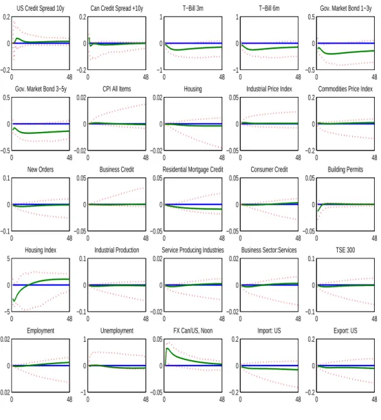
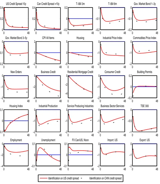
(16) 5.2. Canadian credit shock. In the previous section, we showed that a global credit shock has significant and meaningful effects on the Canadian economy. Now, we will see if a national credit shock, identified using a Canadian external finance premium measure, produces any effect. The recursive scheme is the following:. [U Sspread10y,. CP I,. U R,. M S,. R,. F X,. CAN spread10y].. The credit shock is identified as the last element of εt . This identification is similar to what has been done in structural VAR and in FAVAR frameworks with the US data: activity and price measures do not respond immediately to a credit shock, nor to interest rates or money supply. We also add the exchange rate, considered exogenous to the credit shock7 . Contrary to other studies, we control for the US credit markets by including the US credit spread, but the results do not change if we exclude it. The impulse responses are presented in Figure 3. Overall, the national credit shock does not seem to produce any significant effect on the economy. In particular, the standard deviation of the credit shock in this identification scheme is more than 8 times smaller than in the case of the global credit shock. The previous results suggest that all effects on the Canadian economy are caused by a global (or US) credit shock. Hence, modeling Canada as a closed economy when identifying and measuring the effects of credit shocks can be misleading in the sense that if any effects are found, these are not caused by a national but a global shock. To understand better this phenomenon, we tried another recursive scheme:. [CAN spread10y,. CP I,. U R,. M S,. R,. F X].. Here, the Canadian credit spread is taken to be exogenous to price, activity, money, interest rate and exchange rate measures. Our a priori idea is that the Canadian credit spread is Granger caused by the US spread so that this identification scheme would produce similar results to the first one. In Figure 4 we present the results from these two identification schemes. Overall, they are very similar, except that when using the Canadian spread the effects are slightly more important for some variables. This suggests that the same shock can be identified using either Canadian or US external finance premium 7 Other. orderings were also tried and the results were very similar.. 12.

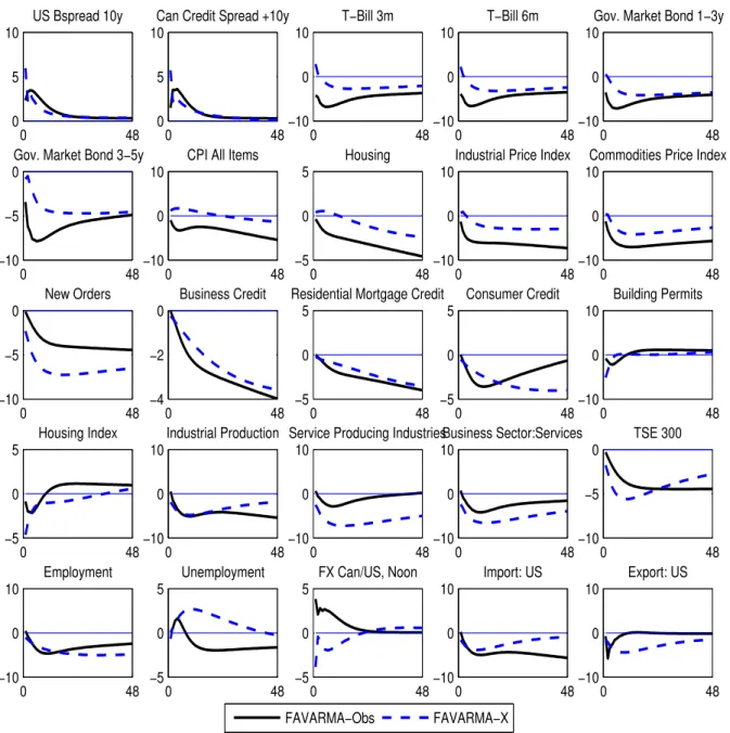
(17) measures. Moreover, the structural factors from the two models are highly correlated (correlation coefficients are higher than 0.9 in absolute value). Finally, we tested the Granger causality between the two credit spreads. The results are reported in Table 3. According to p-values, the hypothesis that the US credit spread does not cause the Canadian credit spread is strongly rejected and there is no evidence to reject the hypothesis that the Canadian credit spread does not Granger cause the US spread. Hence, these results confirm our intuition and suggest that the effects of credit shocks in Canada are essentially caused by unexpected changes in foreign credit market conditions.. 5.3. Further robustness analysis. So far the results confirm our intuition, indicating that Canadian credit conditions are a quasi-deterministic component of American credit conditions (interpreted as global conditions). Thus, it seems that the Canadian credit market is not able to generate shocks. We know that Canadian firms are more liquid than American ones, but their capital structure should not change anything as long as the credit market has been defined here as exogenous to Canadian economy. Our best guess to explain these results seem to be in relation to the size of the Canadian economy and its opening on US economy. But one could ask if we are confident that the insertion of an American credit spread in our database is enough to understand US dynamics? In other words, do we really identify a US credit shock or some global shock to which US economy responds. To answer this question we do two simple robustness analysis and check different identification schemes. The first consider a FAVARMA model with observed factors (US spread), and the second propose an extension of the FAVARMA model by allowing for exogenous variables in factors dynamic.. FAVARMA with observable factors. Xt   Rt    Ft. The model can be written as follows:. = =. ΛFt + νt   R  t−1  Φ(L)   + Θ(L)ηt , Ft−1. (16) (17). where Rt contains M observed factors. In our example, Rt is the US 10-year B-spread. The model is 13.

(18) estimated in the same way as the benchmark specification, with one additional step to impose Rt as observed factor. To do so, we follow the iterative principal approach as in Boivin, Giannoni and Stevanovic (2009):. 1 Initialize Fˆt to be the K first principal components of Xt . ˆ F,j ˆ R,j ˜j ˆ R,0 2 (i) Regress Xt on Fˆt and Rt , to obtain Λ and Λ t t . (ii) Compute Xt = Xt − Λt Rt (iii) Update ˜t. Fˆt as the first K principal components of X. We use the causal ordering in (17 ) to identify the innovation associated to Rt . Hence, the US spread is exogenous to all Canadian factors. The impulse response of all elements in Xt are easily obtained after ˆ inverting (17 ) and premultiplying it by Λ.. FAVARMA-X What if we observe the US credit shock such that it is exogenous to the Canadian economy? A natural thing to do would be to add it as an exogenous variable in the FAVARMA framework. The model becomes:. Xt. =. ΛFt + νt. (18). Ft. =. Φ(L)Ft−1 + βWt + Θ(L)ηt ,. (19). where Wt is the exogenous variable. The estimation proceeds as in Dufour and Stevanovic (2010), with exception that Wt is added to the matrix of regressors during the second step. Here, Wt contains the estimate of US credit shock from Boivin, Giannoni and Stevanovic (2010). Their data set ends on March 2009, so we also restrict our series to end on that period. The advantage of this framework is that the US credit shock has been identified within a US economy model, and then is not subject to the critique that we do not necessary identify the good shock. The impulse response functions after a positive unexpected US credit shock from both models are compared in Figure 5. In both models a VARMA(2,1) has been suggested by the information criterion. We standardized all IRF to have the unit variance, since the impulse shock is not of the same size across models. Hence, the scale is irrelevant, but our interest is to compare the shape and qualitative features of the responses in Figure 5, to IRFs from our benchmark model in Figure 2. We remark that all these specifications and identifications scheme produce quite similar dynamic responses of many variables of interest. Hence, we 14.

(19) believe that the identification procedure in our benchmark model measures the effects US credit shocks in Canada.. 5.4. Interpretation of factors. As it was pointed out in BGS, the procedure to identify the structural shocks can produce interpretable factors8 . Remember that structural shocks are linear combination of residuals, εt = Hηt . Using this hypothesis, we can rewrite the system (10)-(11) in its structural form. Xt. =. Λ? Ft? + ut. Ft?. =. ? Φ? (L)Ft−1 + Θ? (L)εt ,. where Ft? = HFt , Λ? = ΛH −1 , Φ? (L) = HΦ(L)H −1 , and Θ? (L) = HΘ(L)H −1 . Hence, given the estimates ˆ Fˆt . The last six columns in Table of Ft and H, we can obtain an estimate of the structural factors: Fˆt? = H 2 contain the marginal contribution of each structural factor to the total R2 . We can see that the first structural factors mostly explain the two credit spreads. The second is very important for consumer price indexes and housing prices, while the third contributes by completely explaining the unemployment rate. Finally, the fourth factor is important for monetary measures (not reported in the table) and interest rates, while the last two factors do not seem to be interpretable.. 6. Conclusion. In this paper we measured the impact of a credit shock in Canada in a data-rich environment. To incorporate information from a large number of economic and financial indicators, we used a factor-augmented VARMA (FAVARMA) model. The structural shocks were identified by imposing a recursive structure on the impact matrix of the structural MA representation of observable variables. We found that an unexpected increase in the external finance premium on global financial markets, approximated by the US credit spread, generates a significant and persistent economic slowdown in Canada. 8 Note however that factors are identified up to a rotation. Hence, any orthogonal rotation matrix will give the same common component even though the interpretation of each factor in terms of correlation can change.. 15.

(20) Canadian credit spreads rise immediately, while interest rates and credit measures decline. According to R2 results, the common component captures an important dimension of business cycle movements. From the variance decomposition analysis, we observed that the credit shock has an important effect on several economic and financial measures. Another important result is related to the identification of national financial shocks. Previous studies have treated Canada as a closed economy when identifying a credit shock and have found some real effects. Our results suggested however that there is no significant effect of domestic shocks in Canada. Indeed, the effects of credit shocks in Canada are fundamentally caused by the unexpected changes in foreign credit market conditions.. 16.

(21) References [1] Atta-Mensah, J, Dib A. 2008. Bank lending, credit shocks, and the transmission of Canadian monetary policy. International Review of Economics and Finance 17: 159–176 [2] Bai J, Ng S. 2006. Confidence intervals for diffusion index forecasts and inference for factor-augmented regressions. Econometrica 74: 1133–1150. [3] Bai J, Ng S. 2008. Large Dimensional Factor Analysis. Foundations and Trends in Econometrics 3(2): 89–163. [4] Bernanke BS. 1993. Credit in the Macroeconomy. Quarterly Review. Federal Reserve Bank of New York 18: 50–70. [5] Bernanke BS, Gertler M. 1995. Inside the black box: The credit channel of monetary policy transmission. Journal of Economic Perspectives 9: 27–48. [6] Bernanke BS, Gertler M, Gilchrist S. 1999. The Financial Accelerator in a Quantitative Business Cycle Framework. In The Handbook of Macroeconomics. Taylor JB, Woodford M(eds). Elsevier Science B.V. Amsterdam: 1341-1369. [7] Bernanke BS, Boivin J, Eliasz P. 2005. Measuring the effects of monetary policy: a factor-augmented vector autoregressive (FAVAR) approach. Quarterly Journal of Economics 120: 387-422. [8] Bloom N. 2009. The impact of uncertainty shocks. Econometrica 77(3): 623-685. [9] Boivin J, Giannoni MP, Stevanović D. 2009. Monetary Transmission in a Small Open Economy: More Data, Fewer Puzzles. Manuscript. Columbia University. [10] Boivin J, Giannoni MP, Stevanović D. 2010. Dynamic effects of credit shocks in a data-rich environment. Manuscript. Columbia University. [11] Christiano LJ, Motto R, Rostagno M. 2009. Shocks, Structures, or Monetary Policies? The Euro Area and U.S. After 2001. Journal of Economic Dynamics and Control 32: 2476-2506. [12] Diebold FX, Rudebusch GD, Aruoba B. 2006. The Macroeconomy and the Yield Curve: A Dynamic Latent Factor Approach. Journal of Econometrics 131: 309-338. [13] Dufour JM, Pelletier D. 2008. Practical methods for modeling weak VARMA processes: identification, estimation and specification with a macroeconomic application. Working Paper, McGill University. [14] Dufour JM, Stevanović D. 2010. Factor-augmented VARMA models: identification, estimation, forecasting and impulse responses. Manuscript. Université de Montréal. [15] Dynan K, Elmendorf DW, Sichel DE. 2006. Can Financial Innovation Help to Explain the Reduced Volatility of Economic Activity? Journal of Monetary Economics 53: 123. [16] Espinoza RA, Fornari F, Lombardi MJ. 2009. The role of financial variables in predicting economic activity. ECB working paper 1108. [17] Estrella A, Hardouvelis GA. 1991. The term structure as a predictor of real economic activity. Journal of Finance 46(2): 555-76. [18] Forni M, Giannone D, Lippi M, Reichlin L. 2009. Opening the black box: identifying shocks and propagation mechanisms in VAR and factor models. Econometric Theory 25: 1319-1347. [19] Forni M, Hallin M, Lippi M, Reichlin L. 2003. Do financial variables help forecasting inflation and real activity in the euro area? Journal of Monetary Economics 50(6): 1243–1255. [20] Gertler M. Lown CS. 1999. The Information in the High-Yield Bond Spread for the Business Cycle: Evidence and Some Implications. Oxford Review of Economic Policy 15: 132-150. 17.

(22) [21] Gilchrist S, Yankov V, Zakrajˇsek E. 2009. Credit Market Shocks and Economic Fluctuations: Evidence From Corporate Bond and Stock Markets. Journal of Monetary Economics 56: 471-493. [22] Gilchrist S, Ortiz A, Zakrajˇsek E. 2009. Credit Risk and the Macroeconomy: Evidence From an Estimated DSGE Model. Manuscript. Boston University. [23] Mueller P. 2007. Credit Spreads and Real Activity. Manuscript. Columbia Business School. [24] Pesaran H, Schuermann T, Treutler BJ, Weiner SM. 2006. Macroeconomic Dynamics and Credit Risk: A Global Perspective. Journal of Money, Credit and Banking 38(5): 1211–1262. [25] Philippon T. 2009. The Bond Market’s Q. Quarterly Journal of Economics. Forthcoming. [26] Safaei J, Cameron NE. 2003. Credit channel and credit shocks in Canadian macrodynamics - a structural VAR approach. Applied Financial Economics 13: 267–277. [27] Stock JH, Watson MW. 1989 New indexes of coincident and leading economic indicators. NBER Macroeconomics Annual. 351–393. [28] Stock JH, Watson MW. 2002. Forecasting using principal components from a large number of predictors. Journal of the American Statistical Association 97: 1167-1179. [29] Stock JH, Watson MW. 2002. Forecasting Output and Inflation: The Role of Asset Prices. Journal of Economic Literature 41, 788-829. [30] Stock JH, Watson MW. 2005. Implications of dynamic factor models for VAR analysis. Manuscript. Harvard University. [31] Yamamoto Y. 2009. Bootstrap inference for impulse response functions in factor-augmented vector autoregressions. Manuscript. Boston University. 18.

(23) 7 US 10 year Bspread CAN 10 year Aspread. 6. 5. 4. 3. 2. 1. 0. −1 1986M1. 1991M1. 1996M1. 2001M1. 2006M12. Figure 1: Credit spreads used in identification of structural shocks. 19. 2008M11.

(24) US Credit Spread 10y. Can Credit Spread +10y. 0.4. 0.4. 0.2. 0.2. 0. 0 0. 48. T−Bill 3m 1. 0. 0. −1. −1. 0. 48. 0. CPI All Items. −0.2. Gov. Market Bond 1−3y 0 −0.2 −0.4. Gov. Market Bond 3−5y 0. T−Bill 6m. 1. 48 Housing. 0.01. 0.02. 0. 0. 0. 48. 0. 48. Indust. Price Index: All Manuf. Commodities Price Index 0 0.1. −0.01. 0. −0.4 0. 48. −0.01. 0. New Orders. 48. −0.02. Business Credit. 0 −0.02. 0. 48. −0.02. 0. Residential Mortgage Credit. 48. −0.1. 0. Consumer Credit. 48 Building Permits. 0. 0.05. 5. 0.02. −0.02. 0. 0. 0. −0.04 0. 48. −0.04. 0. Housing Index. Industrial Production. 5. 0.05. 0. 0. −5. 0. 48. 48. −0.05. −0.05. 0. 48. Service Producing Industries 0.01. 0. 0. Employment. 48. −0.01. 0. Unemployment. 48. −5. 0. 48. −0.02. 2. 0.05. 0. 0. −2. 0. FX Can/US, Noon. 48. −0.05. 0.1. 0.1. 0. 0. 0. 0. 0. −0.5. 0. 48. −0.05. 0. 48. −0.1. 0. 48 Export: US. 0.05. 48. 0. Import: US. 0.5. 0. 48 TSE 300. 0.01. −0.01. 0. Business Sector:Services. 48. −0.1. 0. 48. Figure 2: Impulse of some variables of interest to one standard deviation global credit shock. 20.

(25) US Credit Spread 10y. Can Credit Spread +10y. T−Bill 3m. T−Bill 6m. Gov. Market Bond 1−3y. 0.2. 0.2. 1. 1. 0.5. 0. 0. 0. 0. 0. −0.2. 0. 48. −0.2. 0. Gov. Market Bond 3−5y. 48. −1. 0. CPI All Items. 48. −1. 0. Housing. 48. −0.5. 0.02. 0.02. 0.05. 0.2. 0. 0. 0. 0. 0. 0. 48. −0.02. 0. New Orders. 48. −0.02. Business Credit. 0. 48. −0.05. 0. Residential Mortgage Credit. 48. −0.2. 0.05. 0.05. 0.05. 0. 0. 0. 0. 0. 48. −0.05. 0. Housing Index. Industrial Production. 5. 0.1. 0. 0. −5. 0. 48. 48. −0.1. −0.05. 0. 48. Employment. 0. 48. Service Producing Industries Business Sector:Services 0.02 0.02. 0. 0. −0.05. 48. −0.02. 0. 0. Unemployment. 48. −0.02. −0.05. 0. 0. FX Can/US, Noon. 48. −0.1. 0.2. 0. 0. 0. 0. 0. 0. 48. −0.05. 0. 48. −0.2. 0. 48 Export: US. 0.2. −1. 0. Import: US. 0.05. 48. 48. 0.1. 1. 0. 0 TSE 300. 0.02. −0.02. 48 Building Permits. 0.05. 0. 0. Consumer Credit. 0.1. −0.1. 48 Commodities Price Index. 0.5. −0.5. 0. Industrial Price Index. 48. −0.2. 0. 48. Figure 3: Impulse of some variables of interest to one standard deviation Canadian credit shock. 21.

(26) US Credit Spread 10y. Can Credit Spread +10y. T−Bill 3m. T−Bill 6m. Gov. Market Bond 1−3y. 0.4. 0.4. 0.2. 0. 0. 0.2. 0.2. 0. −0.1. −0.1. 0. 0. 48. 0. 0. Gov. Market Bond 3−5y. 48. −0.2. 0. CPI All Items. 48. −0.2. 0. Housing. 48. −0.2. 0. 2. 5. 0. 0. −0.1. 0. 0. −1. −1. −0.2. 0. 48. −2. 0. New Orders. 48. −5. Business Credit. 0. 0. −1. −2. −2. −4. 0. Industrial Price Index. 0 48 Residential Mortgage Credit. 0 −2. −2. 0. 48. −2. 48 Commodities Price Index. 0. Consumer Credit. 48 Building Permits. 0. 0.2. −1. 0. −4 0. 48. 0. Housing Index. Industrial Production. 0.1. 0. 0. −1. −0.1. 0. 48. 48. −2. 0 48 Service Producing Industries 0 −1. 0. Employment. 48. −2. 0. Unemployment. 48. −2. 0 48 Business Sector:Services. −0.2. 0. −1. −0.5. 0. FX Can/US, Noon. 48. −1. 0.1. 0. 0. −2. 0. 0. −1. −1. 48. −0.1. 0. 48. −0.1. 0. 48. Identification on US credit spread. −2. 0. 48 Export: US. 0.1. 0. 0. Import: US. 0. −4. 48 TSE 300. 0. −2. 0. 48. −2. 0. 48. Identification on CAN credit spread. Figure 4: Comparison of impulse responses to a credit shock identified by US and Canadian credit spreads. 22.

(27) US Bspread 10y. Can Credit Spread +10y 10 10. 10 5. 5. 0 0 48 0 Gov. Market Bond 3−5y 0 10. −10. 48. −10. −5. −2. 0. 48 Housing Index. 5 0 −5. 48. 48 Housing. 5. 0. 48. 0. −10. −10 0 48 0 48 Industrial Price Index Commodities Price Index 10 10 0. 0. −5. −10 −10 0 48 0 48 0 48 Residential Mortgage Credit Consumer Credit Building Permits 5 5 10 0. 0. 0. −4. −5 −5 −10 0 48 0 48 0 48 0 Industrial Production Service Producing IndustriesBusiness Sector:Services 10 10 10 0 0. 0. 0. CPI All Items. Business Credit 0. −10. Gov. Market Bond 1−3y 10. 0. 0. New Orders 0. −10. 48. 0. 0. T−Bill 6m 10. 0. 0. −5. T−Bill 3m. −10. 0. 0. Employment. 48. −10. 0. 0. Unemployment. 48 FX Can/US, Noon. −10. −5. 0. 48. −10. 5. 10. 10. 0. 0. 0. 0. 0. 48. −5. 0. 48. −5. 0. 48. FAVARMA−Obs. −10. 0. 48 Export: US. 5. 0. 0. Import: US. 10. −10. 48 TSE 300. 48. −10. 0. FAVARMA−X. Figure 5: Comparison of IRFs obtained from FAVARMA-obs and FAVARMA-X models. 23. 48.

(28) Series label SCM2AST(RY) SCM2AMT(RY) SCM2ALG(RY) v122531 v122499 v122501 FYAAAC FYBAAC FYGT1.M FYGT10.M 3 Months A Spread 1 Year A Spread 10 Year A Spread 10 Year B Spread 10 Year A Spread 1 Year B Spread. Table 1: Credit spreads Description Bond Yeld: DEX Capital Overall AA Short Term (% per Annum) Bond Yeld: DEX Capital Overall AA Mid Term (% per Annum) Bond Yeld: DEX Capital Overall AA Long Term (% per Annum) Interest Rate: T-bills 3 Months (% per Annum) Interest Rate:Gov. of Can.marketable Bond, 1-3 years (% per Annum) Interest Rate:Gov. of Can. marketable Bond, over 10 years (% per Annum) Bond Yeld: Moodys AAA Corporate (% per Annum) Bond Yeld: Moodys BAA Corporate (% per Annum) Rate: U.S. Treasury Const. Maturities, 1-Year (% Per Annum, NSA) Rate: U.S. Treasury Const. Maturities, 10-Year (% Per Annum, NSA) Canadian credit spreads SCM2AST(RY) - v122531 SCM2AMT(RY) - v122499 SCM2ALT(RY) - v122501 US credit spreads FYBAAC - FYGT10.M FYBAAC - FYGT10.M FYBAAC - FYGT1.M. 24.

(29) Table 2: Explanatory power of Variance decomposition US Credit Spread 10y 0.8813 CAN Credit Spread 10y 0.6293 T-Bill 3m 0.3947 T-Bill 6m 0.4076 Gov. Market Bond 1-3y 0.4231 Gov. Market Bond 3-5y 0.4088 CPI: all items 0.0214 Housing price index 0.0520 Industrial price index 0.5029 Commodity price index 0.5197 New orders 0.7074 Business credit 0.3425 Residential mortgage credit 0.1982 Consumer credit 0.4595 Building permits 0.1688 Housing index 0.1149 Indust. Prod.: manufact. 0.5726 Indust. Prod.: services 0.6779 Business sector: services 0.6749 TSE 300 0.6659 Employment 0.5691 Unemployment rate 0.0840 FX Can/US 0.0201 Imports: US 0.4857 Exports: US 0.7741 Variables. global credit shock R2 F1∗ 0.4631 1.0000 0.5019 0.7730 0.9603 0.3505 0.9685 0.3739 0.9779 0.4052 0.9717 0.4093 0.9121 0.0313 0.4149 0.0263 0.4942 0.3727 0.3525 0.2383 0.2874 0.5524 0.4045 0.4472 0.6025 0.1181 0.3332 0.0935 0.1184 0.0469 0.8045 0.0640 0.6352 0.3971 0.3501 0.3738 0.3793 0.3894 0.1972 0.3591 0.5161 0.3528 0.8403 0.0465 0.7872 0.0092 0.3276 0.3150 0.4445 0.5063. Table 3: Testing Granger causality H0 US Spread does not Granger cause Can Spread Can Spread does not Granger cause US Spread. and common component Marginal contribution to F2∗ F3∗ F4∗ 0.0000 0.0000 0.0000 0.0003 0.0430 0.0209 0.0281 0.0399 0.5797 0.0254 0.0396 0.5592 0.0206 0.0837 0.4841 0.0183 0.1279 0.4347 0.9687 0.0000 0.0000 0.8049 0.0428 0.0826 0.1894 0.0127 0.1834 0.2580 0.0523 0.2489 0.0012 0.0143 0.2315 0.0000 0.3007 0.0944 0.0310 0.1648 0.3405 0.0025 0.7411 0.0382 0.0381 0.0053 0.2183 0.0009 0.6939 0.0211 0.0002 0.0451 0.3325 0.1041 0.0278 0.3205 0.1336 0.0061 0.3317 0.0773 0.0210 0.3141 0.0081 0.2223 0.1725 0.0049 0.9486 0.0000 0.0084 0.0091 0.1638 0.0142 0.0704 0.2515 0.0082 0.0284 0.3419. between US and Canadian credit spreads F-stat P-value 11.3519 0.0001 1.0326 0.3574. 25. R2 Ft F5∗ 0.0000 0.0518 0.0016 0.0015 0.0022 0.0026 0.0000 0.0066 0.0008 0.0442 0.0696 0.0302 0.3373 0.0350 0.2942 0.2177 0.0784 0.0686 0.0516 0.2109 0.0013 0.0000 0.5601 0.2310 0.1125. F6∗ 0.0000 0.1109 0.0001 0.0005 0.0041 0.0072 0.0000 0.0367 0.2410 0.1583 0.1310 0.1277 0.0083 0.0896 0.3971 0.0024 0.1467 0.1052 0.0876 0.0176 0.2430 0.0000 0.2495 0.1179 0.0028.

(30) Appendix A: Additional results. Regional Responses of CPI in Deviation with respect to National Response. Regional Responses of Unemployment in Deviation with respect to National Response 0.2. 2 0 −2. 0. 0. −0.2. 48. 0. 48. Regional Responses of Employment in Deviation Regional Responses of Building Permits in Deviation with respect to National Response with respect to National Response 2 0.2 0 −2. 0. 0. −0.2. 48. 0. 48. Regional Responses of Housing Starts in Deviation with respect to National Response 0.2 Atlantic Center. 0. Prairies BC. −0.2. 0. 48. Figure 6: Regional impulse responses to a credit shock in deviation with respect to national response. • Atlantic provinces: Newfoundland and Labrador, Prince Edward Island, Nova Scotia and New Brunswick • Center: Québec and Ontario • Prairies: Manitoba, Saskatchewan and Alberta • BC: British Columbia. 26.

(31) Appendix B: Bootstrap procedure The goal is to obtain confidence bands for impulse responses to structural shocks in representation (10-11) with assumption (13). • Step 1 Shuffle the time dimension of the residuals in (11) and resample static factors using estimates of the VARMA coefficients: ˆ ˆ ηt F˜t = Φ(L) F˜t−1 + Θ˜ • Step 2 Shuffle the time dimension of the residuals in (10), and resample the observable series using new factors obtained from the previous step and the estimated loadings: ˜t = Λ ˆ F˜t + u X ˜t • Step 3 ˜ t , identify the structural shock and produce impulse responses. Estimate the FAVARMA model on X As it was pointed out in Dufour and Stevanovic (2010), having a good approximation of the true factor process can be very important in order to get the right bootstrap procedure. If the finite VAR approximation is far away from the truth, and if the finite VARMA representation does much better, allowing for the MA part should provide a more reliable inference.. 27.

(32) Appendix C: Data description The transformation codes (labeled T-Code) are: 1 - no transformation; 2 - first difference; 4 - logarithm; 5 first difference of logarithm.. Canadian Data No.. StatCan no. Code. 1 2 3 4 5 6 7 8 9 10 11 12 13 14 15 16 17 18 19 20 21 22 23 24 25 26 27 28 29 30 31 32 33 34 35 36 37 38 39 40 41 42 43 44 45 46 47 48 49 50 51 52 53 54 55 56 57 58 59 60 61 62 63 64 65. v41690973 v41690974 v41690993 v41691046 v41691051 v41691055 v41691065 v41691066 v41691108 v41691129 v41691153 v41691170 v41692942 v41691232 v41691233 v41691238 v41691237 v41691239 v41691219 v41691222 v41691223 v41691225 v41691229 v41691230 v41691231 v41691244 v41691369 v41691363 v41691367 v41691379 v41691503 v41691497 v41691501 v41691513 v41691638 v41691632 v41691636 v41691648 v41691773 v41691767 v41691771 v41691783 v41691909 v41691903 v41691907 v41691919 v41692045 v41692039 v41692043 v41692055 v41692181 v41692175 v41692179 v41692191 v41692317 v41692311 v41692315 v41692327 v41692452 v41692446 v41692450 v41692462 v41692588 v41692582 v41692586. 5 5 5 5 5 5 5 5 5 5 5 5 5 5 5 5 5 5 5 5 5 5 5 5 5 5 5 5 5 5 5 5 5 5 5 5 5 5 5 5 5 5 5 5 5 5 5 5 5 5 5 5 5 5 5 5 5 5 5 5 5 5 5 5 5. Series category Table 326-0020 Consumer Price Index Canada, Provinces All-items (2002=100) Food (2002=100) Dairy products (2002=100) Food purchased from restaurants (2002=100) Rented accommodation (2002=100) Owned accommodation (2002=100) Natural gas (2002=100) Fuel oil and other fuels (2002=100) Clothing and footwear (2002=100) Private transportation (2002=100) Health and personal care (2002=100) Recreation, education and reading (2002=100) All-items excluding eight of the most volatile components (Bank of Canada definition) (2002=100) All-items excluding food (2002=100) All-items excluding food and energy (2002=100) All-items excluding energy (2002=100) Food and energy (2002=100) Energy (2002=100) Housing (1986 definition) (2002=100) Goods (2002=100) Durable goods (2002=100) Non-durable goods (2002=100) Goods excluding food purchased from stores and energy (2002=100) Services (2002=100) Services excluding shelter services (2002=100) Newfoundland and Labrador; All-items (2002=100) Newfoundland and Labrador; All-items excluding food and energy (2002=100) Newfoundland and Labrador; Goods (2002=100) Newfoundland and Labrador; Services (2002=100) Prince Edward Island; All-items (2002=100) Prince Edward Island; All-items excluding food and energy (2002=100) Prince Edward Island; Goods (2002=100) Prince Edward Island; Services (2002=100) Nova Scotia; All-items (2002=100) Nova Scotia; All-items excluding food and energy (2002=100) Nova Scotia; Goods (2002=100) Nova Scotia; Services (2002=100) New Brunswick; All-items (2002=100) New Brunswick; All-items excluding food and energy (2002=100) New Brunswick; Goods (2002=100) New Brunswick; Services (2002=100) Quebec; All-items (2002=100) Quebec; All-items excluding food and energy (2002=100) Quebec; Goods (2002=100) Quebec; Services (2002=100) Ontario; All-items (2002=100) Ontario; All-items excluding food and energy (2002=100) Ontario; Goods (2002=100) Ontario; Services (2002=100) Manitoba; All-items (2002=100) Manitoba; All-items excluding food and energy (2002=100) Manitoba; Goods (2002=100) Manitoba; Services (2002=100) Saskatchewan; All-items (2002=100) Saskatchewan; All-items excluding food and energy (2002=100) Saskatchewan; Goods (2002=100) Saskatchewan; Services (2002=100) Alberta; All-items (2002=100) Alberta; All-items excluding food and energy (2002=100) Alberta; Goods (2002=100) Alberta; Services (2002=100) British Columbia; All-items (2002=100) British Columbia; All-items excluding food and energy (2002=100) British Columbia; Goods (2002=100) British Columbia; Services (2002=100). 66 67 68 69 70 71 72 73 74 75 76 77 78 79 80 81 82 83 84 85 86 87. v14098 v41651 v13824 v41560 v13859 v41595 v13866 v41602 v13873 v41609 v13880 v41616 v13887 v41623 v13894 v41630 v13901 v41637 v13908 v41644 v13831 v41567. 1 1 1 1 1 1 1 1 1 1 1 1 1 1 1 1 1 1 1 1 1 1. Table 026-0001 Building permits, residential values and number of units Canada; Total dwellings (number of units) [D848383] Canada; Total dwellings (dollars - thousands) [D845521] Newfoundland and Labrador; Total dwellings (number of units) [D847651] Newfoundland and Labrador; Total dwellings (dollars - thousands) [D845363] Prince Edward Island; Total dwellings (number of units) [D847658] Prince Edward Island; Total dwellings (dollars - thousands) [D845370] Nova Scotia; Total dwellings (number of units) [D847665] Nova Scotia; Total dwellings (dollars - thousands) [D845377] New Brunswick; Total dwellings (number of units) [D847672] New Brunswick; Total dwellings (dollars - thousands) [D845384] Quebec; Total dwellings (number of units) [D847679] Quebec; Total dwellings (dollars - thousands) [D845391] Ontario; Total dwellings (number of units) [D847686] Ontario; Total dwellings (dollars - thousands) [D845398] Manitoba; Total dwellings (number of units) [D847693] Manitoba; Total dwellings (dollars - thousands) [D845405] Saskatchewan; Total dwellings (number of units) [D847700] Saskatchewan; Total dwellings (dollars - thousands) [D845412] Alberta; Total dwellings (number of units) [D847707] Alberta; Total dwellings (dollars - thousands) [D845419] British Columbia; Total dwellings (number of units) [D847714] British Columbia; Total dwellings (dollars - thousands) [D845426]. 28.

(33) 88 89 90 91 92 93 94 95 96 97 98. v730040 v729972 v729973 v729974 v729975 v729976 v729981 v729987 v729988 v729989 v729990. 1 1 1 1 1 1 1 1 1 1 1. 99 100 101 102 103 104 105 106 107 108. v7677 v7680 v7681 v7682 v7683 v7684 v7686 v7678 v7679 v7688. 1 1 5 5 5 5 1 5 5 5. Table 027-0002 CMHC, housing starts, under constr and completions, SA Canada; Total units (units - thousands) [J9001] Newfoundland and Labrador; Total units (units - thousands) [J7002] Prince Edward Island; Total units (units - thousands) [J7003] Nova Scotia; Total units (units - thousands) [J7004] New Brunswick; Total units (units - thousands) [J7005] Quebec; Total units (units - thousands) [J7006] Ontario; Total units (units - thousands) [J7008] Manitoba; Total units (units - thousands) [J7011] Saskatchewan; Total units (units - thousands) [J7012] Alberta; Total units (units - thousands) [J7013] British Columbia; Total units (units - thousands) [J7014] Table 377-0003 Business leading indicators for Canada Average work week, manufacturing; Smoothed (hours) [D100042] Housing index; Smoothed (index, 1992=100) [D100043] United States composite leading index; Smoothed (index, 1992=100) [D100044] Money supply; Smoothed (dollars, 1992 - millions) [D100045] New orders, durable goods; Smoothed (dollars, 1992 - millions) [D100046] Retail trade, furniture and appliances; Smoothed (dollars, 1992 - millions) [D100047] Shipment to inventory ratio, finished products; Smoothed (ratio) [D100049] Stock price index, TSE 300; Smoothed (index, 1975=1000) [D100050] Business and personal services employment; Smoothed (persons - thousands) [D100051] Composite index of 10 indicators; Smoothed (index, 1992=100) [D100053]. 109 110 111 112 113 114 115 116 117 118 119 120 121 122 123 124 125 126 127 128 129 130 131 132 133 134 135 136 137 138 139 140 141 142 143. v41881478 v41881480 v41881481 v41881482 v41881485 v41881486 v41881487 v41881488 v41881489 v41881494 v41881501 v41881524 v41881525 v41881527 v41881555 v41881564 v41881602 v41881606 v41881637 v41881654 v41881662 v41881663 v41881674 v41881675 v41881688 v41881689 v41881690 v41881699 v41881724 v41881756 v41881759 v41881776 v41881777 v41881779 v41881780. 5 5 5 5 5 5 5 5 5 5 5 5 5 5 5 5 5 5 5 5 5 5 5 5 5 5 5 5 5 5 5 5 5 5 5. Table 379-0027 GDP at basic prices, by NAICS, Canada, SA, 2002 constant prices All industries [T001] (dollars - millions) Business sector, goods [T003] (dollars - millions) Business sector, services [T004] (dollars - millions) Non-business sector industries [T005] (dollars - millions) Goods-producing industries [T008] (dollars - millions) Service-producing industries [T009] (dollars - millions) Industrial production [T010] (dollars - millions) Non-durable manufacturing industries [T011] (dollars - millions) Durable manufacturing industries [T012] (dollars - millions) Agriculture, forestry, fishing and hunting [11] (dollars - millions) Mining and oil and gas extraction [21] (dollars - millions) Residential building construction [230A] (dollars - millions) Non-residential building construction [230B] (dollars - millions) Manufacturing [31-33] (dollars - millions) Wood product manufacturing [321] (dollars - millions) Paper manufacturing [322] (dollars - millions) Rubber product manufacturing [3262] (dollars - millions) Non-metallic mineral product manufacturing [327] (dollars - millions) Machinery manufacturing [333] (dollars - millions) Electrical equipment, appliance and component manufacturing [335] (dollars - millions) Transportation equipment manufacturing [336] (dollars - millions) Motor vehicle manufacturing [3361] (dollars - millions) Aerospace product and parts manufacturing [3364] (dollars - millions) Railroad rolling stock manufacturing [3365] (dollars - millions) Wholesale trade [41] (dollars - millions) Retail trade [44-45] (dollars - millions) Transportation and warehousing [48-49] (dollars - millions) Pipeline transportation [486] (dollars - millions) Finance, insurance, realestate, rental and leasing and management of companies and enterprises [5A] (dollars - millions) Educational services [61] (dollars - millions) Health care and social assistance [62] (dollars - millions) Federal government public administration [911] (dollars - millions) Defence services [9111] (dollars - millions) Provincial and territorial public administration [912] (dollars - millions) Local, municipal and regional public administration [913] (dollars - millions). 144 145 146 147 148 149 150 151 152 153 154 155 156 157 158 159 160 161 162 163. v1575728 v1575754 v1575886 v1575925 v1575903 v1575934 v1575958 v1575457 v1575493 v1575511 v1575557 v1575610 v3860051 v3822562 v3825177 v3825178 v3825179 v3825180 v3825181 v3825183. 5 5 5 5 5 5 5 5 5 5 5 5 5 5 5 5 5 5 5 5. Tables 329-00(46,38,39) Industrial price indexes, 1997=100 Transformer equipment (index, 1997=100) [P5648] Electric motors and generators (index, 1997=100) [P5674] Diesel fuel (index, 1997=100) [P5806] Light fuel oil (index, 1997=100) [P5845] Heavy fuel oil (index, 1997=100) [P5823] Lubricating oils and greases (index, 1997=100) [P5854] Asphalt mixtures and emulsions (index, 1997=100) [P5878] Industrial trucks, tractors and parts (index, 1997=100) [P5329] Parts, air conditioning and refrigeration equipment (index, 1997=100) [P5365] Food products industrial machinery and equipment (index, 1997=100) [P5383] Trucks, chassis, tractors, commercial (index, 1997=100) [P5429] Motor vehicle engine parts (index, 1997=100) [P5482] Motor vehicle brakes (index, 1997=100) [P5512] All manufacturing (index, 1997=100) [P6253] Total excluding food and beverage manufacturing (index, 1997=100) [P6491] Food and beverage manufacturing [311, 3121] (index, 1997=100) [P6492] Food and beverage manufacturing excluding alcoholic beverages (index, 1997=100) [P6493] Non-food (including alcoholic beverages) manufacturing (index, 1997=100) [P6494] Basic manufacturing industries [321, 322, 327, 331] (index, 1997=100) [P6495] Primary metal manufacturing excluding precious metals (index, 1997=100) [P6497]. 164 165 166 167 168. v36382 v36383 v36384 v36385 v36386. 5 5 5 5 5. Table 176-0001 Commodity price index, US$ (index, 82-90=100) Total, all commodities (index, 82-90=100) [B3300] Total excluding energy (index, 82-90=100) [B3301] Energy (index, 82-90=100) [B3302] Food (index, 82-90=100) [B3303] Industrial materials (index, 82-90=100) [B3304]. 169 170 171 172 173 174 175 176 177 178 179 180. v37412 v37413 v37414 v37415 v37416 v37419 v37420 v122620 v122628 v6384 v6385 v6386. 5 5 5 5 5 5 5 5 1 5 5 5. Tables 176-00(46,47), 184-0002 Stock market statistics Toronto Stock Exchange, value of shares traded (dollars - millions) [B4213] Toronto Stock Exchange, volume of shares traded (shares - millions) [B4214] United States common stocks, Dow-Jones industrials, high (index) [B4218] United States common stocks, Dow-Jones industrials, low (index) [B4219] United States common stocks, Dow-Jones industrials, close (index) [B4220] New York Stock Exchange, customers’ debit balances (dollars - millions) [B4223] New York Stock Exchange, customers’ free credit balance (dollars - millions) [B4224] Standard and Poor’s/Toronto Stock Exchange Composite Index, close (index, 1975=1000) [B4237] Toronto Stock Exchange, stock dividend yields (composite), closing quotations (percent) [B4245] Total volume; Value of shares traded (dollars - millions) [D4560] Industrials; Value of shares traded (dollars - millions) [D4558] Mining and oils; Value of shares traded (dollars - millions) [D4559]. 29.