HAL Id: hal-00512281
https://hal.archives-ouvertes.fr/hal-00512281
Submitted on 29 Aug 2010
HAL is a multi-disciplinary open access
archive for the deposit and dissemination of
sci-entific research documents, whether they are
pub-lished or not. The documents may come from
teaching and research institutions in France or
abroad, or from public or private research centers.
L’archive ouverte pluridisciplinaire HAL, est
destinée au dépôt et à la diffusion de documents
scientifiques de niveau recherche, publiés ou non,
émanant des établissements d’enseignement et de
recherche français ou étrangers, des laboratoires
publics ou privés.
Optimal gathering algorithms in multi-hop radio tree
networks with interferences.
Jean-Claude Bermond, Min-Li Yu
To cite this version:
Jean-Claude Bermond, Min-Li Yu. Optimal gathering algorithms in multi-hop radio tree networks
with interferences.. AD-HocNow 08, Sep 2008, Nice, France. pp.204-217. �hal-00512281�
Optimal gathering algorithms
in multi-hop radio tree-networks with
interferences
Jean-Claude Bermond⋆ and Min-Li Yu⋆⋆
1 MASCOTTE, joint project CNRS-INRIA-UNSA, 2004 Route des Lucioles, BP 93, F-06902 Sophia-Antipolis, France
2 University College of the Fraser Valley, Department of Mathematics and Statistics, Abbotsford, BC, Canada V2S 4N2 [email protected]
Abstract. We study the problem of gathering information from the nodes of a multi-hop radio network into a pre-defined destination node under the interference constraints. In such a network, a message can only be properly received if there is no interference from another message being simultaneously transmitted. The network is modeled as a graph, where the vertices represent the nodes and the edges, the possible com-munications. The interference constraint is modeled by a fixed integer dI ≥1, which implies that nodes within distance dI in the graph from one sender cannot receive messages from another node. In this paper, we suppose that it takes one unit of time (slot) to transmit a unit-length message. A step (or round) consists of a set of non interfering (compat-ible) calls and uses one slot. We present optimal algorithms that give minimum number of steps (delay) for the gathering problem with buffer-ing possibility, when the network is a tree, the root is the destination and dI = 1. In fact we study the equivalent personalized broadcasting problem instead.
1
Introduction
1.1 Problem statement
The problem we consider in this paper was motivated by a question asked by France Telecom about “how to provide Internet connection to a village” (see [6]) and is related to the following scenario. Suppose we are given a set of communication devices placed in houses in a village (for instance, network interfaces that connect computers to the Internet). They require access to a gateway (for instance, a satellite antenna) to send and receive data through a
⋆Partially supported by the CRC CORSO with France Telecom, by the European FET project AEOLUS, and by the INRIA associated team RESEAUXCOM with S.F.U.
⋆⋆ Partially supported by the Natural Sciences and Engineering Research Council of Canada and by the INRIA associated team RESEAUXCOM with S.F.U.
multi-hop wireless network. In this network, the devices communicate exclusively by means of radio transmissions, referred to as calls. A call involves a message and two devices, the sender and the receiver. The communication is subject to the following technological constraints:
Reachability constraint: in order to be reached by a call, the receiver of this call must be within reachability distance of the sender.
Interference constraint: a call may interfere with calls that are in the neigh-borhood of the receiver, or a message can be properly received only if no other senders are in the neighborhood of the receiver.
t-gathering problem: suppose each device of the network has a piece of infor-mation. The t-gathering consists of collecting (gathering) all these pieces of information into a special device t, called the gathering node, by the means of calls subject to the two constraints described before. The t-gathering prob-lem is to realize such a constrained gathering without concatenating mes-sages and with the minimum delay.
An equivalent formulation is the so-called
s-personalized broadcast : here a single device (the gateway in the problem of France Telecom) called source s has a different piece of information to broadcast to every other device in the network by the means of calls subject to the two constraints described before. The s-personalized broadcast is to realize such a constrained gathering without concatenating messages and with the minimum delay.
A slight variation of this problem has received much attention in the context of sensor networks. In such networks, each device contains a sensor and the gathering problem corresponds to the situation where information collected at each sensor has to be gathered to a single central device (base station). However, most of the articles are concerned with minimizing the energy consumption and allow aggregation of data. The work which is most related to ours is [11], in which reachability and interference constraints are also assumed, but most of its results apply for the case of directional antennas.
1.2 Model and assumptions
According to the model adopted in [2], the network described above is repre-sented by an undirected graph G = (V, E), where V is the set of nodes, each of which representing a communication device, and E is the set of edges, represent-ing the pairs of nodes involved in possible calls. There is a special pre-defined node s called the source (sink in the gathering case). Let dG(u, v) indicate the
distance in G, defined as the length of a shortest path between u and v. We model the reachability and the interference constraints by two positive integers, respec-tively dT ≥ 1 and dI ≥ dT. An important case is dT = 1, which means that a
G is the communication graph). The second parameter dI models the
interfer-ence constraint as follows: if a receiver is within distance dI from a sender, then
this node cannot receive any other message. If u sends a message m to v, then the call (u, v) interferes with every node w ∈ V such that dG(u, w) ≤ dI. Two
calls are said to be compatible if they do not interfere with each other (other-wise, they are incompatible). More precisely, two calls (s1, r1) and (s2, r2), for
r1, r2, s1, s2∈ V , are compatible if dG(s1, r2) > dI and dG(s2, r1) > dI. Observe
that one of the consequences of the interference constraint is that s1 6= r2 and
s2 6= r1, which implies that a node is not able to send and receive messages
simultaneously. A step (round) is a set of compatible calls. We assume that ev-ery occurrence of a call takes one unit of time (or one slot) and involves a one unit-length message.We also assume that buffering is possible in intermediate nodes.
In this paper, our aim is to find efficient algorithms that give optimal solutions for the s-personalized broadcast problem when dT = dI = 1 and G is a tree.
1.3 Related work
The broadcasting and gossiping problems have been widely studied for wired networks (see [15]), including models that assume no concatenation of messages (see [4]). For radio networks, the case when dI = 1 is studied only for
broadcast-ing in [10, 12] and gossipbroadcast-ing in [8, 9, 14]. Note that broadcastbroadcast-ing is different from our problem which is personalized broadcasting, as in the process of broadcast, the same information has to be transmitted to all the other nodes and so flood-ing techniques can be used. Recently the gatherflood-ing problem has gained much attention. In [2], assuming an arbitrary size of information in each node, a pro-tocol for general graphs with an approximation factor of at most 4 is presented. It is also shown that the problem of finding an optimal gathering protocol does not admit a Fully Polynomial Time Approximation Scheme if dI > dT, unless
P=NP, and is NP-hard if dI = dT. In the case where each node has exactly one unit of information to transmit (or to receive which is the case we consider), the problem is NP-hard if dI > dT but the complexity is unknown for dI = dT. An
extension of the problem where messages can be released over time is considered in [7] and a 4-approximation algorithm is presented. In [5], optimal solutions are provided for the two-dimensional square grid with dT = 1. In [1] the case of a
path is considered for dT = 1 and any dI. The problem is solved when the sink
(source) is at one end of the path and only partly solved when the sink is in the middle of the path.
As mentioned before, sensor networks have been the subject of many papers. But, most of them deal with minimizing the energy consumption or maximizing the life time of the sensor network. In [11] they minimize the delay but their model is slightly different from ours as each node is equipped with directional antennas and no buffering capacity is available in the nodes. Furthermore they only suppose that a node cannot receive and send simultaneously, and more precisely, this corresponds to the case in our model when dT = 1, interference
at a time. Under their assumptions, they give optimal (polynomial) gathering protocols for path and tree networks. Their work has been extended to general graphs in [13] for unitary messages. In [3], a companion paper to that one, the same problem as ours is considered, but no buffering is allowed. Finally, another related model can be found in [16], where the authors study the case in which steady-state flow demands between each pair of nodes have to be satisfied.
1.4 Main result
In this paper, we deal with the situation when G is a tree T with N vertices and with a source (or root) s and dT = dI = 1 which can be viewed as a
generalization of the results of [11] and [13]. In their case the only constraint is that a node cannot receive and transmit at the same time (which can be viewed as dI = 0). They proved that the minimum number of steps is either N − 1 or
2n1− 1 where n1 is the size of the biggest subtree.
Here we need to consider not only subtrees, but also subsubtrees. Indeed, when dI = 1, two calls in two different branches are incompatible only if they
have the same sender. If two calls (s1, r1) and (s2, r2) in the same path are
incom-patible and the arcs are in the order: s, . . . , s1, r1, . . . , s2, r2, . . ., then d(r1, s2) ≤
1. Otherwise two calls in the same path are compatible if they are separated by at least two arcs.
Here we will have roughly three different forms of trees. Either the tree looks like a path with a big sub-sub-tree formed by the vertices at distance ≥ 2 from s, in which case we will need roughly 3 times the size of this big sub-component. Or the tree has only a big component but inside this component the sub-components are somewhat balanced in which case we need roughly 2 times the size of this big component.In the remaining case (balanced tree an example being a spider (generalized star) we need N − 1 steps.
To state more precisely our main result, let assume that deg(s) = m. Let r1,
r2, ..., rm be the neighbors of s, and Ti be the subtree of T with root ri, where
1 ≤ i ≤ m. The size of Ti is simply |Ti| = ni. Similarly let ri,j be the neighbors
of ri and Ti,j be the subtree with root ri,j. The size of Ti,j will be denoted by
|Ti,j| = ni,j. Furthermore, we will assume that the Ti,j’s are ordered according
to their sizes. So ni,1= max ni,j
Let Mi = max{2ni− 1, ni+ 2ni,1− 1}. For the rest of the paper, subtrees
are ordered according to the values of Mi: M1≥ M2≥ M3≥ . . . ≥ Mm. In case
of equality the order is determined by the sizes.
Theorem 1. When dT = dI = 1 and T is a tree, the minimum number of steps
to complete a personalized broadcasting ( or gathering) is equal to max{N − 1, M1+ ǫ}, where ǫ = 1 if M1= M2 and 0 otherwise.
Although the lower bound is easy to prove and the minimum time can be ex-pressed in a simple formula, in order to obtain optimal algorithms many different situations are needed to be considered and a lot of experiments were performed before the arrival to the final optimal algorithms.
2
Lower bounds and Basic algorithms.
For the rest of the paper we will simply denote by g(T ) (instead of g(T, s, dT, dI)
used in [2] ) the minimum number of steps required to complete the personalized broadcast from s (gathering to s) of one unitary message to each node of T under the interference constraint defined by dI = 1.
2.1 Lower bounds.
Proposition 1. g(T ) ≥ max{N − 1, M1+ ǫ}
Proof. We exhibit different sets of incompatible calls which must be scheduled in different steps (or rounds).
Consider the calls on the arcs (s, ri) and they are all incompatible and there
are N − 1 of them, as this is the number of messages needed to be sent by the source. So N − 1 is a lower bound for g(T ).
Similarly, for each i, the nicalls on the arc (s, ri) and the ni− 1 arcs leaving
ri, are all incompatible. Their number is 2ni− 1. So 2ni− 1 is a lower bound for
g(T ).
Consider also the following incompatible calls : those on the arc (s, ri) and
there are ni of them, the ni,1 calls on the arc (ri, ri,1), and the ni,1− 1 on the
arcs leaving ri,1. Altogether we have ni+ 2ni,1− 1 incompatible calls and this
is also a lower bound for g(T ).
Hence, Mi and therefore M1 is a lower bound. If M1 = M2, then any
algo-rithm starts calling one of r1 or r2 only at step 2 or after, and so it needs at
least M1+ 1 steps.
In the next subsections, we present algorithms that perform personalized broadcasting, which will give optimal solutions when there is only one subtree and will also be used for the general case, in particular when there are two subtrees, by applying them to each subtree. We describe the algorithms for one subtree Ti rooted in ri. We call Tia type 1 subtree if Mi= 2ni− 1. Otherwise,
it is called a type 2 subtree.
2.2 CASE 1: Ti is a subtree of type 1.
We first present an algorithm for a type 1 subtree Ti. In this case recall that
Mi= 2ni− 1.
Let Xt denote the set of vertices to which the source has sent a message
before step t (that is at the end of step t − 1) and let Tt
i be the subtree obtained
from Ti by deleting Xt. Similarly denote by Ti,jt the component obtained from
Ti,j by deleting the vertices of Xt. Let nti= |Tit| and nti,j= |Ti,jt |.
The idea of the algorithm is the following: the source sends every odd step to ria message destinated to a leaf of a big component of Ti, in order to guarantee
that at any step there is no component having more than half of the vertices (or nt
different components of Ti in order to be able to do compatible calls efficiently
in even steps in different components. We first describe the algorithm, then use an example to illustrate it and finally we prove that it is valid and takes Mi
steps (which is the lower bound as Mi≥ N − 1 = ni− 1).
Algorithm A: Personalized broadcasting for a subtree of type 1 At the beginning X1= ∅ and T1
i = Ti.
- During an odd step t = 2k − 1 , k = 1, 2, . . . , ni
Let Tt
i,jk be the largest component of T t
i not chosen at the preceding odd
step (that is jk 6= jk−1) and let xk be a leaf in this component. The source s
sends the message mk for xk on the arc (s, ri). Then we update Xt+1= Xt∪ xk
and Tt+1
i = Tit− xk.
During the odd steps, both ri and the ri,j are inactive.
Finally any vertex at distance ≥ 3 from the source forwards immediately the message received at the preceding step except when it is the destination, in which case the message is stored (if it is mlwith destination xl, then the message
is forwarded to its neighbor on the path to xl).
- During an even step t = 2k , k = 1, 2, . . . , ni− 1
- ri sends to ri,jkthe message mkreceived at step 2k − 1 with the destination
xk in Ti,jt k.
- ri,jk−1 sends the message mk−1(received at step 2k − 2) to its neighbor on
the path to xk−1, except when it is the destination, the message is just stored.
- Any vertex at distance ≥ 3 from the source forwards immediately the message received at the preceding step except when it is the destination, in which case the message is stored.
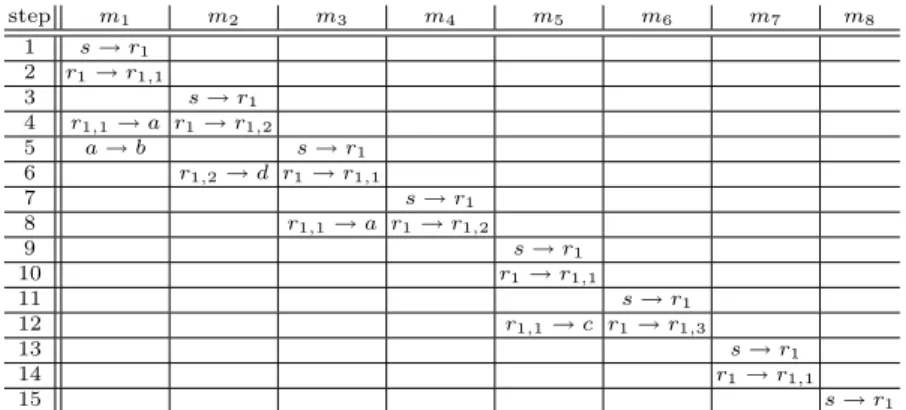
Example: Table 1 illustrates how algorithm A works when it is applied to the type 1 tree given in Fig. 1.
s
r
1b
c
d
r
1 ,3a
r
1 ,1r
1,2s
r
1b
c
d
r
1 ,3a
r
1 ,1r
1 ,2u
w
v
Fig. 1
Fig. 2
step m1 m2 m3 m4 m5 m6 m7 m8 1 s → r1 2 r1→ r1,1 3 s → r1 4 r1,1→ a r1→ r1,2 5 a → b s → r1 6 r1,2→ d r1→ r1,1 7 s → r1 8 r1,1→ a r1→ r1,2 9 s → r1 10 r1→ r1,1 11 s → r1 12 r1,1→ c r1→ r1,3 13 s → r1 14 r1→ r1,1 15 s → r1
Table 1.personalized broadcasting on the tree in Fig.1 with source s using Algorithm A.
Here, N = 9, n1= 8 and n1,1= 4. As M1= 15 = 2n1− 1 = n1+ 2n1,1− 1,
it is a type 1 tree. At step 1, s sends a message destinated to a leaf in T1,1 (the
largest component), for example x1= b (we could have chosen c). So m1= m(b),
the message destinated to b. At step 2, r1sends m1 to r1,1. At step 3, s sends a
message destinated to a leaf in the largest component different from T3
1,1, namely
T3
1,2 and the only choice is x2 = d. At step 4, r1 sends to r1,2 m2 = m(d) and
r1,1 sends m1 to a (its neighbor on the path to b). At step 5, s sends a message
destinated to a leaf in T5
1,1 (the largest component), for example x3 = a (we
could have chosen c). Also a, which is at distance 3 from s, forwards m1 to b
where it is stored. The other steps are described in table 1: we have x4 = r1,2
(we could have chosen r1,3), x5= c, x6= r1,3, x7= r1,1 and x8= r1. Therefore,
m1 = m(b), m2= m(d), m3 = m(a), m4= m(r1,2), m5= m(c), m6 = m(r1,3),
m7= m(r1,1) and m8= m(r1).
Proposition 2. Algorithm A is valid, i.e. all the calls are compatible.
Proof. Consider a call with a sender s and it happens in an odd step. As ri and
ri,j are inactive, only the source is sending among the vertices at distance at
most 2 from s and so this call is compatible with the others calls whose senders are at distance ≥ 3.
Now consider a call with a sender ri and it must happen in an even step.
Suppose it is a call done at step 2k from rito ri,jk. This call is compatible with
the other calls in the component Ti,jk, as they involve senders at distance at
least 4 from s. Indeed the preceding messages in Ti,jk have been sent at step at
most 2k − 4 from ri to ri,jk and at step at most 2k − 2 from ri,jk to a neighbor
and then forwarded. Therefore they either arrived at the destinations or at a vertex with distance at least 4 from s. They are also compatible with the calls in other components as none of them involve ri.
If two calls are in different components Ti,j, then they are compatible as the
with senders in the same component Ti,j are compatible and this follows from
the fact that they are sent by ri,jwithin two steps differing by at least 4, as the
same component cannot be chosen in two consecutive even steps. Because the distance between two such senders is at least 4, the distance between a sender and the other receiver is at least 3 > 1 = dI.
Proposition 3. At the end of the Mi = 2ni− 1 steps of the algorithm A all
the vertices of Ti have received their own messages and so the gathering time is
Mi= 2ni− 1.
Proof. We first prove that at any step there is no component Tt
i,j such that
nt i,j >
nt i
2. Indeed, it is true at step t = 1 as indeed Ti is type 1, 2n 1
i,1 ≤ ni.
Suppose that the property is not true and let t0 = 2k0− 1 be the first step
at which it happens. Then there exists such a component of size strictly bigger than nt0i
2 . Hence, in the two preceding odd steps, this component was the biggest
one and it should have been chosen in one of these two steps, and therefore, this component was already of size bigger than half at step t0− 2 = 2k0− 3 or
t0− 4 = 2k0− 5 contradicting the choice of k0.
Therefore at any step t = 2k − 1 there is a new vertex xk to which a message
can be sent. Hence, all the messages have been sent by the source at end of step Mi= 2ni− 1.
Consider a message mk which is sent by s at step 2k − 1. If k = nithis is the
last message with destination ri and it arrives at step 2ni− 1 = Mi.
Otherwise ri sends mk at step 2k to ri,jk. If ri,jk is its destination, then it
arrives at step 2k ≤ 2ni− 2 < Mi, as k < ni. Otherwise, mk is sent by ri,jk
on the path to xk at step 2k + 2 and then forwarded immediately till it reaches
xk. Let d(s, xk) be the distance between s and xk. Note that d(s, xk) ≥ 3. The
messages with destination on the path from s to xkare all sent after xk(otherwise
we would have not chosen a leaf contradicting the algorithm). Therefore k ≤ ni − d(s, xk) + 1. Finally mk is received by xk at step 2k + d(s, xk) − 1 ≤
2ni− d(s, xk) + 1 ≤ 2ni− 2 = Mi− 1 as d(s, xk) ≥ 3.
2.3 CASE 2: Ti is a subtree of type 2.
Here Mi = ni+ 2ni,1− 1. So there is a component Ti,1such that 2ni,1> ni. The
idea consists in considering a set of vertices Si in this component such that the
subtree T∗
i obtained by deleting them is of type 1 and then to apply algorithm
A to T∗
i = Ti− Si. For the vertices of Si note that, in the formula for Mi, they
are counted for 3. So we will send the messages destinated to them each 3 steps. A natural way will be to send to the vertices of Si during the first 3|Si| steps
of the algorithm: the source sends first a message to them at steps 3h, where 0 ≤ h ≤ ni−n∗i−1 and then the message is forwarded immediately till it reaches
the destination. This algorithm can be also viewed in an inductive fashion: take a leaf u in Ti,1; at step 1, the source sends to ri the message to u and then the
step 4 we apply the algorithm to the tree T − u using either induction or the algorithm A if T − u is of type 1.
This idea works perfectly for one subtree and will be in fact used later for 3 or more subtrees in Section 4.3. But unfortunately it does not lead to a solution in all the cases. For example suppose we have two subtrees. If T1 is of type
1, then the source will send every odd step. Assume that T2 is of type 2 with
M2 = M1− 1; so the source should first send to it at step 2. But then after 3
steps, the source has to send again at step 5. however, s is in fact busy sending to T1 in this step.
So we will proceed in a different manner by first sending to vertices in T∗ i
using Algorithm A, and then use what we call a 3-step extension to send to the rest of vertices by pushing the messages along some paths. So, messages arrive in the leaves only at the last steps of the algorithm. In fact if one thinks in terms of gathering (where the algorithm is the reverse of that for personalized broadcasting) it is more natural to send first the messages from vertices far away that are those from Si= Ti− Ti∗ .
We develop an algorithm that proceeds in 2 phases. In the first phase, each vertex receives an integer label which indicates the step in which this message will be sent by the source in the second phase. Therefore, in the second phase, the source will use the information from the labels given in the previous phase to send the proper message at each step. The algorithm is described below and will then be illustrated by an example. We will prove that it is valid and takes Mi steps (which is the lower bound as Mi ≥ N − 1 = ni− 1).
Algorithm B: Personalized broadcasting for a subtree of type 2 More precisely, let Si be a set of σi vertices of Ti,1 such that, after deletion,
we obtain a tree T∗
i = Ti− Si with n∗i = ni− σi = |Ti∗| vertices. Now Mi∗ =
2n∗
i− 1 = n∗i+ 2n∗i,1− 1 where ni,1∗ = ni,1− σi. Therefore, Ti∗is a type 1 subtree.
Phase 1 : Run the algorithm A on T∗
i, except that the source sends at step
t = 2k −1 just a label of value k (1 ≤ k ≤ n∗
i) (not the message). Then the source
sends successively to each node of Sian unique label (in the range [n∗i+1, . . . , ni])
by using σi times the following ”3-step extension” (3σi more steps). Order the
vertices of Si= {sn∗
i+1+h, 0 ≤ h ≤ ni− n ∗
i− 1} such that the following property
is satisfied: for each h, sn∗
i+1+h is connected to T ∗∪ {s
n∗
i+1, . . . , sn∗i+h}. Hence
there exists a path from s to sn∗
i+1+h, where all the nodes except the last one
(sn∗
i+1+h) have already received a label. Let the vertices of this path be u0 =
s, u1= ri, u2= ri,1, u3, . . . , udh= sn∗i+1+h, where dh= d(s, sn∗i+1+h).
Do the following 3 steps in any order: in one step, do the compatible calls (u3p, u3p+1), in the next step, do the compatible calls (u3p+1, u3p+2) and in the
last one, do the compatible calls (u3p+2, u3p+3).
During each call, each sender (if it is not the source) sends the label it has stored. Therefore at the end of the ”3-step extension” each node has the label of its predecessor on the path. The source sends to ri a new label n∗i + 1 + h.
Note that the calls in an extension are compatible with the calls of any other extension as they are done at different steps.
Note also that the order in which we organize the 3 steps has no importance. However for the purpose of clarity and using in theorem 4, we do the steps in an order such that the source is always sending at an odd step as soon as it becomes possible. So we do the calls (u3p, u3p+1) (including the call with the source as a
sender) at step 2n∗
i + 3h + ǫ, where ǫ = 1 if h is even and 0 if h is odd. Here h
ranges from 0 to σi− 1 = ni− n∗i − 1. We do the calls (u3p+1, u3p+2) at step
2n∗
i+ 3h + (1 − ǫ) and the calls (u3p+2, u3p+3) at step 2n∗i+ 3h + 2. So the source
sends at steps 2n∗
i + 1, 2n∗i + 3, 2n∗i + 7, . . . , 2n∗i + 6q + 1, 2n∗i + 6q + 3, . . . and
is inactive at steps 2n∗
i + 6q + 5.
At the end of the phase 1 of the algorithm, each node has received exactly one unique integer label ranging from 1 to ni. Let xk be the node which has
received the value k.
Phase 2: Run the same algorithm again, but in the first part the source sends at step t = 2k − 1, 1 ≤ k ≤ n∗
i, the message mk destinated to xk, and in the
extensions at step 2n∗
i + 3h + ǫ, where ǫ = 1 if h is even and 0 if h is odd,
the message mn∗
i+1+hto xn∗i+1+h, where 0 ≤ h ≤ ni− n ∗
i − 1. (Another way to
describe this is that in the steps when the source s sends a message, it is m(v) where v contains the smallest label and m(v) has not been sent.).
Example: Consider the type 2 tree given in Fig. 2 obtained by adding three vertices u, v and w and edges (b, u), (u, w) and (c, v) to the tree in Fig.1. Here, n1= 11, n1,1 = 7 and n∗1= 8. Hence, M1= 24 = n1+ 2n1,1− 1(> 21 = 2n1− 1).
Remember that by deleting the vertices u, v and w, the resulting tree is type 1. Now we illustrate algorithm B by applying it to this tree.
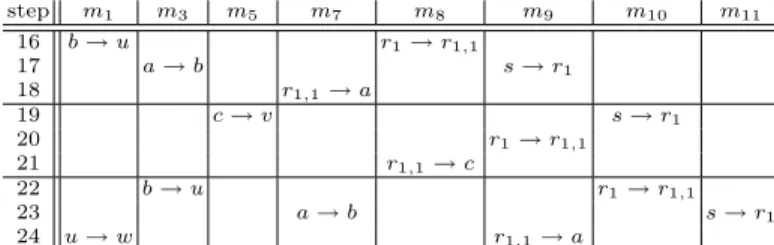
In phase 1, first we apply Algorithm A to the subtree obtained by deleting vertices u, v and w from the given tree (the resulting tree is exactly that of Fig.1), and send a label to each vertex in this subtree, and this takes 15 steps. The resulting labels which are those obtained in the previous example are given in the first row of Table 3. Then 3-step extension is used to extend the labels to the vertices u, v and w. Note that in this process, the labels given in the first part of 15 rounds will be changed. The 3-step extension is illustrated in Table 2 . For example, steps 16, 17 and 18 are used to extend the labeling to the vertex u by moving the labels from s to u along the path (s, r1, r1,1, a, b, u). We need 9
steps to complete the labeling of u, v and w, Table 3 gives the labels of vertices at the end of each 3-step extension in the phase 1 of Algorithm B. The source is not sending at step 21.
Once we have the labels for the vertices, we are able to determine which messages the source should send at different steps. Now we are ready for the second phase of the algorithm. In phase 2, we run again the same algorithm, except this time, instead of labels, at step t = 2k − 1, for 1 ≤ k ≤ 8, the source sends the message m(v), where the label of the vertex v from the first phase of the algorithm is k. For example, s sends m1= m(w) at the first step as x1= w
or the label of w is 1, and sends m2= m(d) at the third step, as x2 = d or the
label of d is 2 and so on. Then s sends at step 17 m(a) as x9 = a, at step 19,
step 16 r1→ r1,1 b → u 17 s → r1 a → b 18 r1,1→ a 19 s → r1 c → v 20 r1→ r1,1 21 r1,1→ c 22 r1→ r1,1 b → u 23 s → r1 a → b 24 r1,1→ a u → w
Table 2.9 steps of 3-step extension to label u, v and w.
r1 r1,1r1,2r1,3 a b c d u v w labels after 15 steps 8 7 4 6 3 1 5 2 - - -labels after 18 steps 9 8 4 6 7 3 5 2 1 - -labels after 21 steps 10 9 4 6 7 3 8 2 1 5 -labels after 24 steps 11 10 4 6 9 7 8 2 3 5 1 names of the vertices x11 x10 x4 x6 x9x7x8x2x3x5x1
Table 3.Labels of vertices after the phase 1 of Algorithm B.
is exactly the same as that of the previous example for the first 15 steps and so they are omitted in the table 4. In fact, the vertices not in T1,1 have received
their messages at the end of the first 15 steps (they are the messages m2= m(d),
m4 = m(r1,2) and m6 = m(r1,3) that have arrived at their destinations). We
indicate in the table 4 the steps of transmission of the other messages Proposition 4. Algorithm B is valid and uses Mi steps (so g(Ti) = Mi).
Proof. The algorithm B is valid as during each step we have only compatible calls (that is the case for algorithm A applied to T∗
i and then the calls of each
step of the extension have been designed to be compatible). At the end of the algorithm each vertex has received its message. In fact, a vertex will receive its message in the first part of the algorithm (before the 3-steps extension) if it is in Ti,j, where j 6= 1, and otherwise, in one of the 3-steps of the last extension. The
algorithm uses 2n∗
i−1 steps in the first part and then 3σisteps for the extensions.
Therefore we have altogether 2n∗
i+ 3σi− 1 = (n∗i+ σi) + (n∗i+ 2σi) − 1 steps. But step m1 m3 m5 m7 m8 m9 m10 m11 16 b → u r1→ r1,1 17 a → b s → r1 18 r1,1→ a 19 c → v s → r1 20 r1→ r1,1 21 r1,1→ c 22 b → u r1→ r1,1 23 a → b s → r1 24 u → w r1,1→ a
n∗
i + σi= ni. By definition of Ti∗, n∗i = 2n∗i,1= 2(ni,1− σi) so n∗i + 2σi = 2ni,1
and so the number of steps is ni+ 2ni,1− 1 = Mi.
3
General Algorithms
We will apply basic algorithms (A or B according to the type of subtrees) first in the case of a single subtree and then of two subtrees. For m ≥ 3, we will use some other techniques and induction; however we will deal first with some special cases. Recall that subtrees are ordered according to the values of Mi:
M1≥ M2≥ M3≥ . . . ≥ Mm. In case of equality the order is determined by the
sizes.
3.1 Case of one subtree.
In that case we apply directly the basic algorithm to the tree and we get Theorem 2. In the case where T consists of one subtree T1, g(T ) = M1> N −1.
3.2 Case of two subtrees.
We apply the basic algorithm to the subtree T1. All the vertices are informed
in M1 steps. We also apply simultaneously the basic algorithm to the subtree
T2, but starting at step 2 ; all the steps are translated by one and therefore all
vertices of T2 are informed in M2+ 1 steps.
Theorem 3. In the case where T consists of two subtrees T1 and T2, g(T ) =
max{M1, M2+ 1} (this value is equal to max{N − 1, M1+ ǫ} where ǫ = 1 if
M1= M2 and 0 otherwise).
Proof. Let us first prove that all the calls are compatible. The validity of Algo-rithm A or B covers the case when two calls belong to the same subtree. That is the case also for the calls having the source as sender; indeed both in algo-rithm A or B the source is sending only during some odd steps. So here the source sends to r1at some odd steps and to r2at some even steps. Finally if two
calls belong to different subtrees and are not both sent by the source, then the distance between one sender and the other receiver is at least 2.
Altogether the algorithm uses max{M1, M2+ 1} = M1+ ǫ steps. We claim
that M1+ ǫ ≥ N − 1, which will prove that the lower bound is attained in that
case. The claim is true if M1≥ N −1. If M1≤ N −2, then 2n1−1 ≤ M1≤ N −2
and 2n2−1 ≤ M2≤ N −2. (1) That implies n1+n2≤ N −1. But N −1 = n1+n2
and therefore there are equalities everywhere in (1); that is n1= n2=N −12 and
3.3 General case: m > 2
Due to lack of space the proofs are omitted in this section. Complete proofs can
be acessible via the webpage of the first author (http://www-sop.inria.fr/mascotte/personnel/Jean-Claude.Bermond/). We first deal with a special case
Theorem 4. Suppose T consists of at least 3 subtrees such that T1 and T2 are
of different types and M1≥ N − 1 and M2= M1− 1. Then g(T ) = M1.
Then, for the case m > 2, when we are not in the special case of the preceding theorem 4, we apply induction on N and present algorithms which complete the personalized broadcasting in the number of steps that meet the lower bound. Therefore, the exact number of g(T ) is determined. We will suppose that the source sends at steps 1 and 2 to two different subtrees. Furthermore, if M1 ≥
N − 1 and T1 is of type 1, the algorithm used to send messages to T1 is the
basic algorithm A (in particular the source will send to r1in all odd steps). We
assume that N > 4 otherwise it is trivial and we will distinguish 3 cases getting the following theorems.
Theorem 5. Suppose T consists of at least 3 subtrees and N − 1 > M1. Then
g(T ) = N − 1.
Theorem 6. Suppose T consists of at least 3 subtrees and M1≥ N − 1 and T1
is of type 2. Then g(T ) = M1+ ǫ.
Theorem 7. Suppose T consists of at least 3 subtrees and M1≥ N − 1 and T1
is of type 1. Then g(T ) = M1.
4
Conclusion
In this paper, we present efficient algorithms that give optimal solution for the gathering problem with buffering possibility, when the network is a tree with dI = 1. It should be noted that in our algorithms, the size of our buffers never
exceeds 1. However with such a small buffer, we can in some cases decrease siderably the gathering time comparing to the non buffering assumption con-sidered in [3]. An extension would be to consider a non uniform distribution of messages. Our algorithm can be easily extended to the case where a node receives or sends w(u) > 0 messages ; indeed it suffices to replace a vertex with w(u) messages by w(u) vertices with one message. However if w(u) is allowed to be 0, then the problem will become much more complicated.
It would also be interesting to investigate this problem for different value of dI or some other structures of networks. In particular it is still an open question
to decide if the problem is polynomial for trees in general.
5
Acknowledgments
We would like to thank all the persons who help us with fruitful discussions in particular L. Gargano, A. Liestman, J. Peters and S. Perennes.
References
1. J-C. Bermond, R. Corrˆea, and M. Yu. Gathering algorithms on paths under inter-ference constraints. In 6th Coninter-ference on Algorithms and Complexity, LNCS 3998, pages 115–126, Roma, Italy, May 2006.
2. J-C. Bermond, J. Galtier, R. Klasing, N. Morales, and S. P´erennes. Hardness and approximation of gathering in static radio networks. Parallel Processing Letters, 16(2):165–183, 2006.
3. J-C. Bermond, L. Gargano, and A.A. Rescigno. Gathering with minimum delay in tree sensor networks. In SIROCCO 2008, volume 5058 of Lecture Notes in
Computer Science. Springer-Verlag, June 2008.
4. J-C. Bermond, L. Gargano, A.A. Rescigno, and U. Vaccaro. Fast gossiping by short messages. SIAM Journal on Computing, 27(4):917–941, 1998.
5. J-C. Bermond and J. Peters. Efficient gathering in radio grids with interference. In AlgoTel’05, pages 103–106, Presqu’ˆıle de Giens, May 2005.
6. P. Bertin, J-F. Bresse, and B. Le Sage. Acc`es haut d´ebit en zone rurale: une solution ”ad hoc”. France Telecom R&D, 22:16–18, 2005.
7. V. Bonifaci, P. Korteweg, A. Marchetti-Spaccamela, and L. Stougie. An approxi-mation algorithm for the wireless gathering problem. In L. Arge and R. Freivalds, editors, SWAT, volume 4059 of Lecture Notes in Computer Science, pages 328–338. Springer-Verlag, 2006.
8. M. Christersson, L. Gasieniec, and A. Lingas. Gossiping with bounded size mes-sages in ad-hoc radio networks. In Proc. of ICALP’02, volume 2380 of Lecture
Notes in Computer Science, pages 377–389. Springer-Verlag, 2002.
9. M. Chrobak, L. Gasieniec, and W. Rytter. Fast broadcasting and gossiping in radio networks. Journal of Algorithms, 43(2):177–189, 2002.
10. M. L. Elkin and G. Kortsarz. Logarithmic inapproximability of the radio broadcast problem. Journal of Algorithms, 52(1):8–25, 2004.
11. C. Florens, M. Franceschetti, and R. McEliece. Lower bounds on data collection time in sensory networks. IEEE Journal on Selected Areas in Communications, 22(6):1110–1120, 2004.
12. I. Gaber and Y. Mansour. Centralized broadcast in multihop radio networks.
Journal of Algorithms, 46(1):1–20, 2003.
13. L. Gargano and A. Rescigno. Optimally fast data gathering in sensor networks. In R. Kr´aloviˇc and P. Urzyczyn, editors, Proc. of MCFS’06, volume 4162 of Lecture
Notes in Computer Science, pages 399–411. Springer-Verlag, 2006.
14. L. Gasieniec and I. Potapov. Gossiping with unit messages in known radio net-works. In Proceedings of the IFIP 17th World Computer Congress, pages 193–205. Kluwer, B.V., 2002.
15. J. Hromkovic, R. Klasing, A. Pelc, P. Ruzicka, and W. Unger. Dissemination
of Information in Commmunication Networks: Part I. Broadcasting, Gossiping, Leader Election, and Fault-Tolerance. Springer Monograph. Springer-Verlag, 2004. 16. R. Klasing, N. Morales, and S. P´erennes. Complexity of bandwidth allocation in