The Dynamics of Industry Investments

Texte intégral

(1)2007s-09. The Dynamics of Industry Investments Marcel Boyer, Pierre Lasserre, Michel Moreaux. Série Scientifique Scientific Series. Montréal Avril 2007. © 2007 Marcel Boyer, Pierre Lasserre, Michel Moreaux. Tous droits réservés. All rights reserved. Reproduction partielle permise avec citation du document source, incluant la notice ©. Short sections may be quoted without explicit permission, if full credit, including © notice, is given to the source..

(2) CIRANO Le CIRANO est un organisme sans but lucratif constitué en vertu de la Loi des compagnies du Québec. Le financement de son infrastructure et de ses activités de recherche provient des cotisations de ses organisations-membres, d’une subvention d’infrastructure du Ministère du Développement économique et régional et de la Recherche, de même que des subventions et mandats obtenus par ses équipes de recherche. CIRANO is a private non-profit organization incorporated under the Québec Companies Act. Its infrastructure and research activities are funded through fees paid by member organizations, an infrastructure grant from the Ministère du Développement économique et régional et de la Recherche, and grants and research mandates obtained by its research teams. Les partenaires du CIRANO Partenaire majeur Ministère du Développement économique, de l’Innovation et de l’Exportation Partenaires corporatifs Alcan inc. Banque de développement du Canada Banque du Canada Banque Laurentienne du Canada Banque Nationale du Canada Banque Royale du Canada Bell Canada BMO Groupe financier Bombardier Bourse de Montréal Caisse de dépôt et placement du Québec Fédération des caisses Desjardins du Québec Gaz de France Gaz Métro Hydro-Québec Industrie Canada Investissements PSP Ministère des Finances du Québec Pratt & Whitney Canada Raymond Chabot Grant Thornton State Street Global Advisors Ville de Montréal Partenaires universitaires École Polytechnique de Montréal HEC Montréal McGill University Université Concordia Université de Montréal Université de Sherbrooke Université du Québec Université du Québec à Montréal Université Laval Le CIRANO collabore avec de nombreux centres et chaires de recherche universitaires dont on peut consulter la liste sur son site web. Les cahiers de la série scientifique (CS) visent à rendre accessibles des résultats de recherche effectuée au CIRANO afin de susciter échanges et commentaires. Ces cahiers sont écrits dans le style des publications scientifiques. Les idées et les opinions émises sont sous l’unique responsabilité des auteurs et ne représentent pas nécessairement les positions du CIRANO ou de ses partenaires. This paper presents research carried out at CIRANO and aims at encouraging discussion and comment. The observations and viewpoints expressed are the sole responsibility of the authors. They do not necessarily represent positions of CIRANO or its partners.. ISSN 1198-8177.

(3) The Dynamics of Industry Investments* Marcel Boyer †,Pierre Lasserre‡, Michel Moreaux§ Résumé / Abstract Nous étudions le développement d'un duopole dans un modèle en temps continu d'investissement en capacité sans engagement des firmes quant à leurs actions futures. Bien que les unités de capacité soient coûteuses, indivisibles, durables et de taille non négligeable par rapport au marché, l'entrée hâtive ne peut conférer d'avantage durable et à partir d'un certain niveau de développement du marché, les deux firmes sont en activité. Nous évaluons les options réelles d'investissement dans ce contexte. Initialement, le seul équilibre Markovien parfait (ÉMP) est un équilibre de préemption dans lequel le premier investissement en capacité se produit plus tôt et comporte un risque plus élevé que socialement désirable. Une collusion tacite pour retarder les augmentations de capacité subséquentes peut devenir possible en ÉMP. La volatilité du marché et sa vitesse de croissance jouent un rôle crucial : l'émergence d'équilibres de collusion tacite est favorisée par une volatilité plus grande, une croissance plus rapide et un taux d'intérêt ou d'actualisation plus faible. Mots clés : options réelles, duopole, préemption, collusion, investissement en bloc. We study the development of a duopoly in a continuous-time model of capacity investment under no commitment by firms regarding future actions. While capacity units are costly, indivisible, durable, and large relative to market size, early entry cannot secure a first-mover advantage and both firms are active beyond some level of market development. We evaluate the investment real options in that context. In the early industry development phase, the sole Markov Perfect Equilibrium (MPE) is a preemption equilibrium with the first industry investment occurring earlier (hence being riskier) than socially optimal. Once both firms hold capacity, tacit collusion, taking the form of postponed capacity investment, may occur as a MPE. Volatility and the expected speed of market development play a crucial role in competitive behavior: we show that the emergence of tacit collusion equilibria is favored by higher demand volatility, faster market growth, as well as by lower discount rate. Keywords: real options, duopoly, preemption, collusion, lumpy investment Codes JEL : C73, D43, D92; L13 *. We are grateful to Bruno Versaevel of EM Lyon and participants in the Real Options Conferences at Georgetown University (Washington) and EDC (Paris), the Conference in honor of Claude Henry in Paris, as well as in economic theory seminars at USC and Penn State for their comments. Financial support from CIRANO, CIREQ, SHRCC (Canada) and INRA (France) is gratefully acknowledged. † Bell Canada Professor of Industrial Economics, Université de Montréal, marcel.boyer@umontreal.ca. ‡ Department of Economics, Université du Québec à Montréal, lasserre.pierre@uqam.ca. § Institut Universitaire de France, IDEI and LERNA, Université de Toulouse I, mmichel@cict.fr..

(4) 1. Introduction “Real life” investment games played between competing firms in oligopolistic markets typically share the following characteristics. The environment (demand, information and knowledge, supply of inputs) is uncertain in many ways and evolves over time. The investment units come in finite discrete sizes, that is, investments are indivisible and lumpy. Undoing an investment strategy is costly, that is, investments are in part irreversible. Capacity is built or technology adoption is achieved in multiple discrete and separable steps engaged at different times without commitments as to future actions or investment levels and timing. As capacity is built over many periods, firms keep producing and competing, that is, their long term and short term decisions are intertwined. Firms have some (endogenous) flexibility to adapt the course of their investment strategy to exogenous changes in their environment as those strategies are implemented. At the industry level, investments come in waves, with all firms investing simultaneously, or in sequences, with firms investing at different times. Typically, investment (capacity building) games eventually come to an end as the relevant market matures. Although uncertainty is a common feature of the economic modeling of investment games, other stylized facts are less frequently modelled. Typical models assume that firms make a unique decision and must live with that decision afterwards. Such models include models of technology adoption, models of entry, and numerous forms of two stage models where firms first make and commit to long term decisions (stage one) before competing in short term decisions (stage two). Using a strategic real option approach, we develop a model of investment decision making incorporating some of the stylized features identified above: uncertainty, indivisibility, irreversibility, flexibility, dynamic choices of capacity building, no commitments on future actions and strategies, endogenous end to the investment game, and both investment waves and sequential investment timings over time. The analysis of strategic considerations, in a game theoretic sense, is still in its infancy and should be high in the real option research agenda.1 The real option approach 1 Among investment evaluation methods, the real option approach is reaching advanced textbook status and is rapidly gaining reputation and influence among practitioners. Although both academics and practitioners warn against its sometimes daunting complexity, they also stress its unique ability to take account of flexibility in managing ongoing projects, which is a significant but often neglected. 1.

(5) emphasizes the irreversibility, hence indivisibility, of investments.2 Indivisibility often imply a limited number of players, hence imperfect competition. Yet, while it is often stressed that the real option approach is best to analyze investments of strategic importance — the word ’strategic’ appears repeatedly in the real option literature — the bulk of that literature involves decision makers confronted with a stochastic but non-reacting nature rather than reacting competitors.3 The present paper extends the recent contributions in different ways while bringing to bear the older literature on strategic investment,4 in addressing issues such as the role of investment decisions in shaping the structure of a developing sector, the emergence of preemption with rent equalization and dissipation5 versus tacit collusion with rent maintenance, the existence or not of a first-mover advantage,6 , and the effect of strategic competition on real option exercise rules.7 We consider dynamic investments without commitment in an homogeneous product duopoly where rival firms face market development uncertainty and invest in lumpy increments of capacity. Typically, firms hold investment options. We find optimal exercise rules and determine the value of the corresponding options as well as of the firms holding them. source of value. 2 Henry (1974) and Arrow and Fisher (1974) were precursors of the approach. In his treatment of the cost benefit analysis of a “new circumferential highway” around Paris, Claude Henry showed that using the Simon-Theil-Malinvaud certainty equivalent approach “will here, systematically and unduly, favor irreversible decisions, for example, destroying the forests and building the highway.” 3 There are notable exceptions. Grenadier (1996) uses a game-theoretic approach to option exercise in the real estate market; Smets (1995) provides a treatment of the duopoly in a multinational setup, which serves as a basis for the oligopoly discussion in Dixit and Pindyck (1994, pp. 309-14); Lambrecht and Perraudin (1996) and Décamps and Mariotti (2004) investigate the impact of asymmetric cost information on firms’ investment strategies; Baldrusson (1998) considers a duopoly model where firms make continuous incremental investments in capacity showing that when firms differ in size initially, substantial time may pass until they are of the same size; Grenadier (2002) provides a general solution approach for deriving the equilibrium investment strategies of symmetric firms, in a CournotNash framework, facing a sequence of investment opportunities with incremental capacity investments, showing that competition may destroy in part the value of the option to wait; Weeds (2002), Huisman (2001), Huisman and Kort (2003) study option games in a technology adoption context; Boyer et al. (2004) study a duopoly with multiple investments under Bertrand competition; Smit and Trigeorgis (2004) discuss different strategic competition models in the context of real options. 4 Most notably Gilbert and Harris (1984), Fudenberg and Tirole (1985), and Mills (1988). 5 As in Fudenberg and Tirole (1985). 6 As in Gilbert and Harris (1984) or Mills (1988). 7 The recent synthetic work of Athey and Schmutzler (2001) brings some generality and clarity to our understanding of the role of investment in market dominance. They show in particular that, when firms are farsighted and not committed to strategic investment plans, there is little hope to obtain definitive predictions outside specific models.. 2.

(6) Our main results are as follows. Two types of equilibria may arise. In preemption equilibria, which always exist, firms invest at different market development thresholds, hence at different times. In “tacit collusion” equilibria, which only exist under some conditions, firms invest at the same market development threshold, hence simultaneously, and thus such equilibria correspond to “investment wave” equilibria. In preemption equilibria, rents are equalized and partly dissipated while in tacit collusion equilibria, firms exercise market power by implicitly agreeing to postpone their respective investments in capacity building. If firms have equal positive capacities, then the preemption equilibrium exhibits different but uniquely determined market development investment thresholds, hence uniquely specified but stochastic investment timings with either firm moving first. If firms have different capacities and end game conditions are close to be met, the smaller firm acts as first mover. When they exist, tacit collusion or investment wave equilibria are typically numerous and Pareto superior to preemption equilibria from the firms’ viewpoint. Tacit collusion is more profitable when firms have equal capacity in the sense that, when tacit collusion equilibria exist, the joint investment (stochastic) date that maximizes combined profits is an equilibrium if and only if firms are of equal size. Moreover, firms may be able to tacitly collude at some stages of market development but not at others. Low initial capacities are of particular interest in the case of emerging sectors. When at least one firm has no capacity, preemption is the sole equilibrium as tacit collusion cannot then be enforced since the firm the firm cannot be threatened with the loss of an existing rent. Hence, even though the (preemption) equilibrium is characterized by the presence of only one active firm at first, the initial development of the industry is highly competitive as rents are equalized and partly dissipated. Paradoxically, once both firms are active, the industry may become less competitive as tacit collusion equilibria become possible. It is well known that higher volatility raises the value of investment options because a flexible decision maker can achieve higher exposure to upside movements and lower exposure to downside ones. In a strategic setup, higher market volatility also favors also the emergence of tacit collusion equilibria. Similarly, higher expected market growth as well as a lower cost of capital favor the emergence of tacit collusion equilibria. Hence, our results suggest that investment waves (joint investment timings) may signal the exercise. 3.

(7) of market power and are more likely when firms have similar positive capacities, market growth is high, volatility is high, and/or interest rates are low. After presenting the model, the competition framework, and the investment game in Section 2, we proceed in Section 3 with the analysis of essentially all possible industry development histories, more specifically with the explicit analysis of three different situations that essentially cover all relevant ones. We conclude in Section 4. Detailed proofs are provided in the Appendix.. 2. The model. 2.1. Industry characteristics. We consider the development of an industry where demand is affected by multiplicative random shocks. The inverse demand function at time t ≥ 0 is given by: P (t, Xt ) = Yt D−1 (Xt ),. (1). where Xt ≥ 0 is aggregate output, Yt ≥ 0 is a random shock, and D : IR+ → IR+ is the. non-stochastic component of demand. Assumption 1. Demand D(·) is strictly decreasing, continuously differentiable and integrable on IR+ and D(0) = limp↓0 D(p) < ∞; the mapping x 7→ xD−1 (x) is strictly concave on (0, D(0)); aggregate shocks (Yt )t≥0 follow a geometric Brownian motion: dYt = αYt dt + σYt dZt. (2). with Y0 > 0, α > 0, σ > 0, and (Zt )t≥0 a standard Brownian motion with respect to the complete probability space (Ω, F, P ).8. Firms are risk neutral and discount future revenues at the same rate r > α. Investment. takes place in a lumpy way. Each capacity unit costs I, which is constant over time, 8. Thus market demand is driven by consumers’ tastes for the output, not by replication of the initial consumers as in Gilbert and Harris (1984).. 4.

(8) produces at most Q = 1 unit of output, does not depreciate, and has no resale value. 2.2. Competition, output, and investment. We consider a duopoly. At any date t, firms first take their investment decisions and then compete in quantities (à la Cournot) subject to capacity constraints.9 Specifically, within the instant [t, t + τ ), the timing of the game is as follows: (i) first, each firm f chooses how many capacity units νtf to invest in, given the realization of the demand shock Yt and the existing capital stocks (ktf , kt−f ); (ii) next, each firm selects an output level within its capacity, xft ≤ ktf + νtf ; (iii) last, market price is determined according. to (1), with Xt = xft + x−f t .. The specification of inverse demand (1) implies that the short-run Cournot game is independent of the realization of the current industry-wide shock. We can assume that, in the absence of capacity constraints, this game has a unique equilibrium (xc , xc ). Let kc = dxc e be the minimum capital stock required to produce xc . It is then easy to. check that, with given capacities kf ≤ k −f , only three Cournot equilibrium outcomes can occur: (i) both firms are constrained, so that xf = kf and x−f = k−f ; (ii) the. smaller firm is constrained, so that xf = kf , while the bigger firm is not and reacts optimally by choosing x−f on its reaction function; (iii) both firms are unconstrained, so that xf = x−f = xc . The corresponding instantaneous profit of a firm with capacity k when its competitor holds. capacity units can be conveniently denoted Yt πk , where. πk depends on capacities only. 2.3. Markov strategies. A key assumption of our model is that firms cannot (credibly) commit to future investment and output decisions. The game typically generates several investments occurring in endogenous order at endogenous dates. There is no commitment by the firms with respect to their role as first or second investor or to the number of units they will acquire. The natural equilibrium concept here is the Markov perfect equilibrium (MPE), in which firms’ investment and output decisions at each date depend only on the firms’ capital stocks measured in capacity units, (kf , k −f ), as well as on the current level of 9 See Boyer et al. (2004) for a related preemption model with instantaneous competition in prices (Bertrand).. 5.

(9) the industry-wide shock y. This rules out implicit collusion between firms when deciding on output: at each date, and given their current capacities, firms play the unique equilibrium of the static Cournot game described above. Our definition of Markov strategies and of the resulting payoffs is in line with the Fudenberg and Tirole (1985) concept of mixed strategies for timing games in continuous time. The main difference is that, while they focus on deterministic environments, demand fluctuates randomly in our model.10 The basic idea is to construct an adequate continuous time representation of limits of discrete time mixed strategy equilibria by defining a strategy for firm f as a function sf specifying the intensity sfν f (kf , k −f , y) ∈. [0, 1] with which firm f invests in ν f capacity units given the capital stocks (kf , k −f ) and. the industry-wide shock Yt = y. Given a strategy profile (sf , s−f ), U(sf f ,s−f ) (k f , k −f , y) denotes firm f ’s expected discounted profit in state (kf , k −f , y).11 In the rest of the paper, we will omit firm and strategy profile indices in the expression of value functions when no ambiguity arises. 2.4. Firm valuation. Since (Yt )t≥0 is a time homogenous Markov process, an outcome may be described as an ordered sequence of investment triggers together with the short-run instantaneous profits of both firms Yt πk and Yt π k between investments. Let yij (with yij = yji ), where i and j refers to the firms’ capacities immediately before Yt reaches yij for the first time,12 denote the value of Yt that triggers a new investment when total industry capacity is i + j. If the game is over, then yij = ∞. 10 A precise definition of Markov strategies and payoffs under uncertainty can be found in Boyer et al. (2004, Appendix A). 11 The important intuitions that our paper will convey can be grasped in terms of pure strategies. However, in symmetric cases, there will be situations where two pure strategy equilibria exist, where either firm invests first and the other firm second, for identical payoffs. Then there is a possibility, if firms use pure strategies, of both firms investing simultanously by mistake, a sort of coordination failure. Indeed, a firm prefers to invest if its opponent does not but prefers not to invest if its opponent does. Hence both firms wish to avoid the worst of all cases, namely simultaneous investments. Under the foregoing definition of Markov strategies, strategies can be designed such that no entry mistakes P can occur. In the first symmetric MPE we construct in the Appendix, sf1 (0, 0, y P ) = s−f 1 (0, 0, y ) = 0, f −f f −f P where k = k = 0, ν = ν = 1, and y is the level of Yt that triggers the first firm investment in the equilibrim. This acts as a correlation device: each firm is equally likely to invest in state (0, 0, y P ), but the probability of simultaneous entry is zero. This formally jsutifies the usual less rigorous approach consisting in determining at random a (lucky) first mover. 12 Since capacity units do not depreciate, higher triggers along a given development path correspond to higher industry capacity levels: yij ≤ yk ⇔ i + j ≤ k + .. 6.

(10) Suppose Yt = y and let us consider, for simplicity, investments of one single capacity unit only (ν = 1), as investments in multiple capacity units can be treated as oneunit investments occurring at the same time. Let L (i, j, y) denote the current value of the firm of capacity i if it carries out an investment immediately, while its opponent has capacity j. Let F (i, j, y) be the current value of the firm of capacity i when its competitor with capacity j carries out an investment immediately. Let S (i, j, y) denote the current value of the firm of capacity i, with its competitor holding capacity j, if both firms make a simultaneous investment at some future date when Yt reaches say yij . The following lemma gives analytical expressions for the L, F , and S functions. The expressions are divided into a first part corresponding to the current investment and a second part corresponding to the continuation of the game. The latter part is not fully specified at this stage; it will be determined recursively by backward induction, starting from the ‘horizon’, defined in state space as the first (stochastic) time a situation (or capacity combination) is reached such that it is certain that no more investment will take place. Lemma 1 let Yt = y. The value of the firm of capacity i, when it invests immediately while the firm of capacity j does not, is given by the following, where k = i + 1: πkj y−I + L (i, j, y) = r−α where β = 12 − α/σ 2 +. µ. y ykj. ¶β ∙ ¸ πkj c (k, j, ykj ) − ykj r−α. q (α/σ 2 − 12 )2 + 2r/σ 2 > 1 and c (k, j, y) is the continuation value. of the same firm at the time of the next industry investment, if any.. Its value, when it stays put while its competitor of capacity j invests now, is given by the following, where k = j + 1: πik y+ F (i, j, y) = r−α. µ. y yik. ¶β ∙ ¸ πik c (i, k, yik ) − yik . r−α. Its value, when both firms invest simultaneously at some future trigger value yij , is. 7.

(11) given by the following, where k = i + 1 and πij y+ S (i, j, y) = r−α. µ. y yij. ¶β µ. = j + 1:. πk − πij yij − I r−α. ¶. +. µ. y yk. Consider the expression for L (i, j, y). The first part. ¶β ∙ ¸ πk yk . c (k, l, yk ) − r−α πkj y r−α. − I gives the expected. net present value of the profit flows achieved by increasing capacity from i to k = i + 1 at a cost of I, assuming that no more investment is made. The second part ³ ´β £ ¤ πkj y ) − y c (k, j, y adjusts the first one for the effect of subsequent investkj kj ykj r−α. ments, that is for the (equilibrium) exercise by both firms of their investment options. ³ ´β may be viewed as a discount factor defined over the state space rather Indeed, yyij. than the time space13 and the function c (k, j, ykj ) is the continuation value function when. Yt = ykj .14 The expressions for F (i, j, y) and S (i, j, y) can be similarly understood. 2.5. Endgame conditions. Although the investment game imposes no restrictions on capacities, we can characterize endgame conditions: the investment game is over if and only if it is known with certainty that no firm will ever invest in additional capacity. The following proposition gives two conditions, one necessary, one sufficient, for the investment game to be over. Proposition 1 The investment game is over only if (necessity) either condition A or condition B is satisfied, implying that both firms hold a strictly positive capacity; more³ ´β The expression yyij gives the expected discounted value when Yt = y of receiving one dollar the first time Yt reaches yij > y, the length of time necessary to go from y to yij being random. If there is no subsequent investment, so that yij = ∞, the second term in L vanishes. 14 To emphasize that c is a continuation function by definition, L (i, j, y) can be written as " ¶β µ ¶# µ ¶β µ πkj πkj y y L (i, j, y) = −I + c (k, j, ykj ) , + y− ykj r−α ykj r−α ykj 13. where. ∙. πkj r−α y. −. ³. y ykj. ´β ³. πkj r−α ykj. ´¸. is the expected present value of a random annuity Yt πkj lasting. between today (when Yt = y) and the random date at which Yt will reach ykj . Suppose that the investment occurring at ykj is made by the firm with capacity j and no further industry investment occurs afterwards. Then at ykj , the new profit flow of the firm of capacity k becomes πk(j+1) Yt and π c (k, j, ykj ) is the expected present value of that profit flow, namely k(j+1) r−α ykj . The value function L (i, j, y) is then completely defined, provided the trigger value ykj has been determined: L (i, j, y) = ³ ´β πk(j+1) −πkj πkj y y − I + ykj . r−α ykj r−α. 8.

(12) over, the investment game is over if (sufficiency) Condition A is satisfied: (A) Neither capacity constraint is binding in the short-run Cournot game, that is, kf ≥ kc = min{k ∈ IN | k ≥ xc }, f ∈ {1, 2}. (B) Both capacity constraints are binding in the short-run game and would remain binding in case of a unit investment by any one firm. Proposition 1 indicates (i) that no firm can keep its opponent out of the market in the long run, and (ii) that a firm cannot use excess capacity in order to maintain a dominant position in the long run.15 Condition (A) falls short of implying equal capacities for both firms. However it implies that, if capacities are not equal at the end of the game, the number of units used by each firm is the same. If capacities are not equal, some capacity is idle. Condition (A) is not necessary; however if it is not satisfied at the end of the game, Condition (B) must hold. That condition pertains to tacit collusion. It describes a situation where each firm could still profitably increase its capacity if its rival did not react. For such a situation to last forever (game over), it must be the case that firms restrict capacity, hence output, in equilibrium. Such an equilibrium can hold only if any deviation is adequately punished. Condition (B) describes a situation where a firm can inflict a punishment on its competitor if the latter deviates. If the former firm were no longer capacity constrained following an investment by its opponent (Condition (B) not satisfied), then it would not be able to retaliate to the deviation. It is then certain that the opponent would invest at some date t. The ability to retaliate is however not sufficient to sustain a tacit collusion equilibrium. We characterize below the conditions under which the retaliatory power is sufficient to offset the gain from deviating. If the firm to be punished is small, it does not lose as much from an increase in the capacity of its opponent as if it were bigger. This implies that retaliation, hence collusion, is likely 15. The conditions spelled out in Proposition 1 are not compatible with the situation found in Gilbert and Harris (1984) where, in equilibrium, one duopolist concentrates the totality of industry capacity, while the other firm holds no capacity. Their result can be traced to a technical assumption, claimed to be “trivial in that both firms will earn zero profits on new investments in a preemption equilibrium” (p. 206), that gives a first-mover advantage to one firm in order to rule out (mistaken) simultaneous investments. The strategies and equilibrium concept defined above avoid the necessity of any asymmetric treatment.. 9.

(13) to be easier between firms of similar size and explains why the investment game cannot be over unless both firms hold strictly positive capacities. In what follows, firm asymmetry can only take the form of differences in current capacities and may be thought of as inherited from past moves in the industry development game. As discussed above, Lemma 1 provides only a partial characterization of value functions under alternative investment strategies. Completing the characterization requires knowledge of the continuation function c (·) and the appropriate trigger values. These can be determined when the game between the two firms is sufficiently near its end, in the sense of Proposition 1. Once the continuation value function is known in such situations, it is possible to characterize recursively the value function corresponding to previous steps.. 3. Industry development Industry development proceeds by successive capacity acquisitions by one of the firms or both. The particular demand function we use guarantees that the number of capacity units that will eventually be installed is finite and that the industry development game has an end. This is in contrast with most papers on related subjects (investment games; R&D games, etc.) where it is assumed either that the players play only once or that the game goes on indefinitely. Industry development possibilities may be represented as a tree whose nodes give the number of capacity units held by each firm (Figure 1). While the figure indicates possible sequences of capacity investments, it does not provide any indication about the speed at which investments occur and nodes are reached.16 16 In particular this representation is compatible with a firm acquiring more than one unit simultanously, or with both firms investing simultaneously, in which case no time is spent on intermediary nodes.. 10.

(14) (k0 + 3, k 0 + 1) (k 0 + 2, k 0 + 1). ... (k0 + 1, k 0 + 1) (2, 0) ... (k0 , k 0 + 1) (1, 0) % (0, 0) &. % &. (0, 1). .... .... &. (k0 , k 0 + 2). %. .... &. (k 0 + 1, k 0 + 2). (k0 + 2, k 0 + 2). % &. (k 0 , k 0 + 3). %. .... &. (1, 1). % &. &. % &. %. %. (k0 + 1, k 0 + 3). (k0 , k 0 + 4) .... (0, 2) ... .... (k + 1, k). .... ... (k, k). (k + 2, k) %. %. &. &. %. (k, k + 1). &. (k + 1, k + 1). (k, k + 2). Figure 1: Industry capacity development tree We characterize the capacity acquisition path and the competition intensity prevailing at various stages of market and industry development: first, in the early stage when firms hold no capacity (Case 1); second, at a later stage, when firms hold symmetric (Case 2) or asymmetric (Case 3) capacities due to the unraveling of their respective investment strategies. We first consider situations that are “near” the end of the game: from the nodes considered, a limited number of investments will lead to a situation where the investment game is over in the sense of Proposition 1. Once these investment developments are characterized, the previous relevant investment histories can be obtained by backward induction: a limited number of investments will lead to a situation or node from which the (not necessarily unique) unraveling of the investment game has been characterized till endgame conditions are met. Once we have characterized those situations that are “near” the end of the game, we generalize the analysis (in section 3.4) to arbitrary nodes in the industry development tree. Hence, we virtually consider all relevant cases as the path to such characterizations is clearly beaconed. 11.

(15) 3.1. Case 1: No existing capacity. We start with a situation where initial capacities are zero; let us assume that the market is such that unconstrained firms would produce at most one unit each in Cournot duopoly, that is: Assumption 2 0 < xc ≤ 1. Although this assumption allows the monopoly output to exceed unity, so that the acquisition of more than one unit may be considered by any one firm, it also implies that, if both hold one unit or more, the game is over by Proposition 1. Assumption 2 also implies that, whatever the (strictly) positive number of capacity units held by its opponent, a firm obtains instantaneous profit Yt π11 once it invests in one unit or more; consequently it will typically not acquire more than one unit. Therefore, the payoff from not investing immediately is (with π1ν = π11 by Assumption 2) F (0, 0, y) =. µ. y y0ν. ¶β µ. ¶ π11 y0ν − I , r−α. where ν is the number of units acquired by the opponent before the firm acquires its first and single unit. The stopping problem faced by the firm is then:. F ∗ (0, 0, y) = sup y0ν. "µ. y y0ν. ¶β µ. π11 y0ν − I r−α. ¶#. (3). with solution: ∗ ∗ = y01 = y0ν. r−α β , ∀ν ≥ 1. I π11 β − 1. (4). Knowing this, the value for the competitor of acquiring at least one unit immediately ∗ can be at Yt = y, and any number of further units before Y reaches the threshold y01. computed explicitly. For example if it acquires one unit immediately and abstains from. 12.

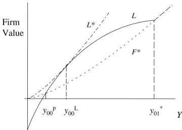
(16) any further investment its value is, according to Lemma 1:17 π10 y−I + L (0, 0, y) = r−α where. π11 ∗ y r−α 01. µ. y ∗ y01. ¶β. π11 − π10 ∗ ∗ y , y < y01 . r − α 01. (5). ∗ = c (1, 0, y), since no more investment is forthcoming beyond y01 by Propo-. sition 1. Similarly, if the investment in the first unit is to take place in the future at y00 > y, then the value of the firm is:. L(0, 0, y00 ) =. µ. y y00. ¶β µ. π10 y00 − I r−α. ¶. +. µ. y ∗ y01. ¶β µ. ¶ π11 − π10 ∗ . y r − α 01. (6). Its maximum L∗ (0, 0, y) with respect to y00 is reached at: y00L =. r−α β I . π10 β − 1. (7). Figure 2 illustrates the functions L (0, 0, y), L∗ (0, 0, y) and F ∗ (0, 0, y).. 17. We leave to the reader the straightforward task to adapt the formula and the rest of the argument ∗ for any number of units acquired by the first investor before the other one invests at y01 . For example if 0 0 ∗ the firm plans to acquire a second new unit at some y , y ≤ y < y01 , the candidate value for L (0, 0, y) ³ ´β h i ³ ´β π10 π20 −π10 0 π21 −π20 ∗ 0 ∗ is r−α y − I + yy0 y − I + yy∗ r−α r−α y01 , y ≤ y < y01 where π21 = π11 by Assumption 01 2. If this value is higher than (5), then it gives the correct expression for L (0, 0, y); if it is lower, then (5) is the appropriate expression. Note that the number of candidates to try is low as it cannot exceed the monopoly capacity under Assumption 2.. 13.

(17) L. Firm Value. L*. F*. y00p y00L. y01*. Y. Figure 2: Firm values under alternative strategies. ∗ It is straightforward to check from (3)—(6) that, within the interval (0, y01 ), there p p such that for y < [>, =]y00 , L(0, 0, y) < [>, =]F (0, 0, y), with exists a unique value y00 p p = inf{t ≥ 0 | Yt ≥ y00 }. the corresponding stochastic stopping time being τ00. We now determine the firms’ equilibrium strategies before any firm has invested, p , investing is for both firms a strictly that is, in states of the form (0, 0, y). If y < y00 ∗ , delaying investment any further is also a strictly dominated strategy while for y ≥ y01 p ∗ ≤ y < y01 , it is dominated strategy. To determine the equilibrium outcome when y00. helpful to consider what would happen if one of the firms were protected from preemption. and could thus choose its optimal stand-alone investment date as a monopoly.18 Given a current industry-wide shock y, the maximal expected payoff that this firm could then achieve by taking the lead is L∗ (0, 0, y). This is strictly higher than F ∗ (0, 0, y).19 In an MPE, however, such a value gap cannot be sustained. If a firm anticipates that its rival L L , then the former is better-off preempting the latter at y00 − dy. will first invest at y00. p L and y00 . When the industry-wide shock Yt is equal This is true for any y between y00 p , the value of both firms is the same, so each firm is indifferent between investing to y00 ∗ , at the immediately and letting its rival invest while waiting to invest until Yt reaches y01 18. Katz and Shapiro (1987). Everything happens as if the firm is myopic and takes no account of the future entry of the follower. This is is line with Leahy (1993): when computing its optimal stand-alone date, a myopic firm overstates by the same amount the value of the investment option and the marginal benefit from investing, leaving the investment rule unaffected. 19. 14.

(18) ∗ ∗ stochastic time τ01 = inf{t ≥ 0 | Yt ≥ y01 }. The following proposition is a transposition. of Fudenberg and Tirole (1985, Proposition 2A) in a stochastic context.. p , Proposition 2 (Preemption equilibrium) Under Assumptions 1 and 2, if Y0 ≤ y00. 1. There exists only one MPE outcome of the investment game: one firm invests at p ∗ , while the other firm waits until τ01 to invest; both times are stochastic. τ00. 2. Rents are equalized to the value of the second investor given by (3). The preemption MPE is characterized by intense competition. The first capacity unit p L < y00 , reflecting a is installed earlier than under protection from preemption since y00. partial dissipation of monopoly rents (Posner, 1975, Fudenberg and Tirole, 1987).. 3.1.1. Socially optimal investment timings. It is more difficult to compare the MPE outcome with the social optimum. Specifically, let k 0 = dD(0)e be the minimum capital stock required to produce D(0). The social. planner’s problem is to find an increasing sequence of stopping times that solves: (. Ey. sup τ1 ≤···≤τk0. " k0 Z X k=1. τk+1. e−rt Yt. τk. Z. k. D−1 (q)d q. 0. #). ,. where by convention τk0 +1 = ∞. Standard computations imply that it is optimal for the. social planner to invest in the first capacity unit when Yt reaches the investment trigger y O such that: y. O. Z. 1. D−1 (q) dq =. 0. β (r − α)I. β−1. p L L . Since y00 < y00 as well, there is no obvious way to compare y O and Clearly, y O < y00 p . y00. However, modifying slightly the model allows an unambiguous comparison between the MPE outcome and the social optimum, thus identifying the key factors involved in a general comparison. Indeed, suppose that the inverse demand curve is a step function, D−1 (Q) = D−1 (dQe); because of the assumption of unit capacity increments, the steps correspond to capacity levels, so that each capacity unit produces at full scale once 15.

(19) installed.20 Then π10 = D−1 (1) =. R1 0. L D−1 (q) dq, so that y00 = y O . It follows that. p < y O , so that the first capacity unit is introduced too early in an MPE, relative to y00. the social optimum. This happens because rents accruing to each firm must be equalized in an MPE, while, from a social point of view, each successive capacity unit yields less value than the preceding one as the consumers’ marginal willingness to pay decreases. In order for the first capacity unit to yield no more rent than the second unit in equilibrium, the first investor must therefore waste resources to compensate for interim earnings so that its value does not exceed that of the second investor. The result that the first industry investment occurs earlier under duopoly than in the social optimum does not depend on the market size assumption k c = 1. As π11 = R2 D−1 (2) = 1 D−1 (q)dq, the second investor introduces the second capacity unit at the. socially optimal date. Since it acts like a monopoly with respect to the market residual demand and since it does not hold any capacity, it will invest as soon as the market is able to support a second capacity unit. However, if the firm that makes the last industry investment already held some capacity, it would postpone its investment in order not to cannibalize its demand. We will show that this is indeed the case. 3.2. Case 2: Symmetric capacities. Let us now investigate the role of existing capacity, starting in this section with situations where firms have identical capacities, as illustrated by the subgame starting at node (k, k) in Figure 1. As in the previous subsection, we will assume that the firms hold a capacity lower than the unconstrained short-run Cournot output, which implies that both firms are initially capacity constrained and that a firm remains constrained if its opponent invests: Assumption 3 0 < xc − k ≤ 1 Assumption 3 is compatible with an unconstrained monopoly output exceeding k +1, so that it does not rule out investments exceeding one unit, allowing a firm to get ahead by more than one unit. It does imply that the end of the game is not too far in the The assumption D−1 (Q) = D−1 (dQe) reduces the consumer surplus by the triangles between the initial inverse demand curve and the steps of the new inverse demand curve, located entirely below the former. In an industry involving indivisible capacity units the same assumption of a stepwise demand would be necessary to ensure that perfect competition coincides with the social optimum. 20. 16.

(20) sense that, by Proposition 1, the game is over once both firms have acquired at least one more unit. To simplify exposition, we take k = 1. Then Assumption 3 implies that π21 > π11 , π22 > π12 , and πν2 = π22 = π2ν , ∀ν ≥ 2. When considering a new investment, firms will now take into account the consequences on the profits they derive from their existing capacity. We will show that, as a result of the cannibalism effect, tacit collusion equilibria may exist besides the preemption equilibrium, provided that either late joint investment or no more investment dominates preemption over the whole relevant market development range.. 3.2.1. The preemption MPE. The investment game with symmetric capacities always has a MPE. Assume that one of the firms has taken the lead by acquiring at least one new unit, bringing its total capacity to ν ≥ 2. For its rival, whatever the number of units held by the first investor, it is a dominant strategy by Assumption 3 to acquire one and only one unit at the. market development threshold determined by the following optimal stopping problem: for y < y1ν , ". π1ν F ∗ (1, ν, y) = sup y+ r−α y1ν. µ. y y1ν. ¶β µ. π22 − π1ν y1ν − I r−α. ¶#. ,. (8). that is, at: ∗ = y1ν. r−α β . I π22 − π1ν β − 1. (9). The situation is similar to the case with no initial capacity except that the trigger value, at which the second investor invests, depends on the number ν of units held by the initial investor. The higher ν, the earlier the second investor will invest because its profits π1ν while waiting are lower the higher ν. The firm that invests first, whether it acquires one single unit or more units, understands all implications of its investment(s) on the behavior of its competitor, so that L (1, 1, y) can be computed explicitly. For example if the early investor acquires only. 17.

(21) ∗ one unit, its payoff at the current level of y ≤ y1ν is, for ν = 1:. π21 y−I + L (1, 1, y) = r−α. µ. y ∗ y12. ¶β µ. ¶ π22 − π21 ∗ . y r − α 12. (10). As before, if the firm were able to choose the investment threshold in the absence of any threat of preemption, the maximum L∗ (1, 1, y) with respect to y, for ν = 1, would be reached at:21 L y11 =. r−α β . I π21 − π11 β − 1. L But under a preemption threat, the firm cannot wait until Yt reaches y1ν and invests p , at which rents are equalized. The following result then parallels at trigger level y1ν. Proposition 2. Proposition 3 (Preemption with equal capacities) Under Assumptions 1 and 3, the investment game has a preemption MPE such that any one firm invests when Yt reaches p ∗ while the other firm invests when Yt reaches y1ν . y1ν. In this equilibrium, the threat of preemption leads to rent equalization and thus to the complete dissipation of any first-mover advantage. However, with positive capacities, the preemption equilibrium may not be the sole type of MPE, as we shall now see.. 3.2.2. Tacit collusion MPE. The fact that the firms hold strictly positive capacities gives rise to the possibility of a different type of MPE . The strategies involved consist in coordinating on a random joint investment date or in abstaining from investing forever. We call these strategies tacit collusion strategies as they imply an increase of firms’ values above the preemption equilibrium level. Note that short-run output decisions are still determined according to Cournot competition. Collusion is achieved only through firms’ investment strategies and not through production decisions. This implies that the only way firms can sustain a ∗ Again the reader can adapt the candidate expressions for L (1, 1, y), with y1ν given by (9), for any new capacity purchase exceeding one unit (ν > 2). The highest such candidate gives L (1, 1, y). It is certain to exist because, as shown in the proofs, the candidate for L corresponding to ν = 1 exceeds ∗ F ∗ (1, 1, y) for some range of y values lower than y12 . 21. 18.

(22) tacit collusion outcome is by investing simultaneously, rather than at different times, and s ∗ exceeding y12 . Indeed if one of the firms were to invest in a by doing so at a threshold y12 ∗ , the latter’s unique optimal continuation strategy second capacity unit at some y < y12 p ∗ . This can be a MPE only if y = y12 as shown in the analysis of would be to invest at y12. the preemption MPE characterized above. Since simultaneous investments of one unit imply by Assumption 3 that both firms then hold more capacity than the unconstrained Cournot output, they will not acquire more than one unit. Furthermore the game is then over by Proposition 1. Suppose that the firms could commit to invest simultaneously at some random future date or to abstain from investing forever. Given a current industry-wide shock y, the expected payoff that they could achieve in this way is, according to Lemma 1: π11 y+ S (1, 1, y) = r−α. µ. y s y11. ¶β µ. ¶ π22 − π11 s y −I . r − α 11. (11). s s∗ If π22 > π11 , S (1, 1, y) has a maximum with respect to y11 , denoted S ∗ (1, 1, y), at y11 :. s∗ = y11. r−α β r−α β ∗ > y12 , I = I π22 − π11 β − 1 π22 − π12 β − 1. (12). s∗ s∗ = inf{t ≥ 0 | Yt ≥ y11 } as the corresponding investment (stochastic) timing. If with τ11. π22 ≤ π11 , S (1, 1, y) attains a maximum of. π11 y r−α. s∗ by letting y11 = ∞ (tacit collusion by. s∗ s∗ = ∞. Clearly if L (1, 1, y) exceeds S ∗ (1, 1, y) at any y ≤ y11 , inaction), in which case τ11. tacit collusion is not an equilibrium since each firm then has an incentive to deviate and invest earlier. Hence, Proposition 4 (Tacit collusion with equal capacities) Under Assumptions 1 and 3, if p , Y0 ≤ y11. 1. A necessary and sufficient condition for the existence of a tacit collusion MPE ∗ is L (1, 1, y) ≤ S ∗ (1, 1, y) ∀y < y12 . If this inequality is strict for all such y,. there exists a continuum of tacit collusion MPE, indexed by their joint investment. s s∗ ∗ s∗ in a range [y s , y11 ], where y12 ≤ y s ≤ y11 . triggers y11. 2. Rents are equalized in each tacit collusion MPE and exceed the preemption MPE rents; the Pareto optimal tacit collusion MPE corresponds to the joint profits max19.

(23) imizing investment rule under the constraint that firms invest simultaneously if they do.22 In this joint-profit maximization tacit collusion MPE, each firm invests in one capacity unit with intensity:. sf1 (1, 1, y) = s−f 1 (1, 1, y) =. ⎧ ⎪ s∗ ⎪ 0 if y ∈ [0, y11 ), ⎪ ⎪ ⎨. ⎪ ⎪ ⎪ ⎪ ⎩ 1 if y ∈ [y s∗ , ∞). 11. 3. If π22 > π11 , the Pareto optimal tacit collusion MPE has both firms investing when s∗ ; otherwise it is such that neither firm ever invests. Yt reaches y11. Propositions 2 and 4 highlight the role of existing capacity in the exercise of market power. A firm that holds no capacity has no incentive to restrain output and thus tacit collusion cannot exist if one firm has zero capacity (Proposition 2).23 Moreover, the mere existence of an incentive to tacitly collude is not enough to guarantee that tacit collusion is sustainable: firms must also follow investment strategies such that a deviation from the tacit collusion outcome would trigger a reaction leading to a new equilibrium with a lower value for the deviating firm. This “punishment” is made difficult because our assumption of a Cournot production equilibrium in any period implies that restraining output can only be achieved by postponing capacity investments in the industry. It follows in particular that the joint investment trigger in any tacit collusion equilibrium must be higher than both triggers in the MPE characterized in Proposition 3. Moreover, a firm becomes more vulnerable to a deviation by its competitor once the trigger value p and for the first investment in the preemption equilibrium has been crossed: once y > y11. until y reaches the threshold for the second investment, a deviation yields the defector a higher rent L (·) than the rent F ∗ (·) obtained by its competitor who would then invest ∗ . Therefore, the rents S ∗ (·) under tacit collusion MPE must be attractive optimally at y12 ∗ . enough (Proposition 4(b)) to beat such defection at any level of y preceding y12 22 Absent that constraint, joint profits maximization would involve sequential investments. As mentioned above, such an investment sequence cannot be sustained as an MPE outcome of our duopoly model, as it would generate a strictly higher expected payoff for the first investor and would therefore be subject to preemption. 23 In the language of contestability, this says that the level of contestability is stronger when the contesting firm is not yet active.. 20.

(24) Proposition 4 provides a necessary and sufficient condition for tacit collusion MPEs to exist. This condition implies restrictions on the components of L (1, 1, y) and S ∗ (1, 1, y): first, the four profit values πij determined by the non-stochastic component of demand D (·) under Cournot competition; second, the parameters underlying real option values, that is, the value of β as determined by the discount rate r as well as the drift α and the volatility σ of the stochastic demand shock process. ∗ e (β, I) = {(π11 , π12 , π22 , π21 ) | E (y; I, β) = S ∗ (1, 1, y) − L (1, 1, y) ≥ 0 ∀y < y12 } Let Λ. e (β, I) is the set of πij quadruples for which tacit collusion equilibria exist given β and (Λ. I); the following proposition states that this set is non empty, is independent of I (that e (β, I) = Λ(β)), and is larger in industries with higher volatility, faster growth and is, Λ lower cost of capital (that is, Λ (β 0 ) ⊂ Λ (β) iff β < β 0 ).. Proposition 5 (Tacit collusion: existence) Under Assumptions 1 and 3: 1. There exists a set of market parameters guaranteeing the existence of tacit collusion MPE. 2. This set is independent of the investment cost I of a capacity unit. 3. It is larger, the higher demand volatility, the faster market growth, and/or the smaller the discount rate. As we know from the real option literature, increased volatility raises the option value of an irreversible investment under no preemption threat: the firm increases its investment threshold to reduce the probability that the stochastic process reverts to undesirable levels after the firm has invested. The flexibility to do so increases the value of the firm; the more so, the higher the volatility. Such an effect is also present here. But there is another effect of volatility: an increase in volatility raises firm values more in a tacit collusion equilibrium than in the preemptive equilibrium, thus favoring the emergence of the former. The reason comes from both timing and discounting. Tacit collusion equilibria involve higher investment thresholds (longer delays), while an increase in volatility amounts to a lower discount rate (recall that β decreases with volatility σ) because it raises the probability that a given threshold value of y be reached in any given amount of time. Although instantaneous profits are always independent of β, the discounted value of the profit flows corresponding to each equilibrium does depend on 21.

(25) ³. y s y11. ´β. β: the (state space) discount factors used in (11) and (10) are respectively and ³ ´β y s ∗ and since y11 > y12 , the former increases more than the latter when β decreases, y∗ 12. that is, when volatility increases. To put it differently, the benefits of restraining supply through delaying investments occur in a distant future, that is, in a higher state of. market development, while the benefits from deviating occur in the immediate future. Other things equal, more volatility gives relatively more weight to the former than to the latter, contrary to conventional wisdom whereby increased volatility, because it warrants a risk premium, amounts to an increase in the discount rate. The intuition for the role of the (time) discount rate and the market growth rate is similar: a lower discount rate favors future payoffs and a larger expected growth rate raises future prospects relative to immediate ones. Hence, both favor the emergence of tacit collusion equilibria through a lower β. 3.3. Case 3: Different capacities. While we have shown that existing capacity is a necessary condition for tacit collusion between identical firms, capacity is also often said to play a role as a barrier to entry and thus can be used as a way to acquire and maintain a dominant position or a first-mover advantage. We assume now that firms differ in their initial sizes. Referring to Figure 1, we now investigate investment subgames such as the game starting at node (k 0 , k 0 + 1) and contrast them with sub-games such as the game starting at node (k, k) analyzed in the previous section. We showed that, with symmetric capacities, there are two possible types of MPE : the preemption equilibrium and the tacit collusion equilibrium. The former always exists, is highly competitive and involves rent equalization. The latter exists under some conditions, provides higher rents to both firms, and also involves rent equalization. We will show that some of these characteristics are modified under asymmetric capacities: initial capacity asymmetry prevents rent equalization in equilibrium and makes collusion more difficult in the sense that joint profits maximization is not compatible with a MPE. Without loss of generality, suppose that one firm holds k0 , k 0 ≥ 1, capacity units. while the other holds k 0 + 1 units, that k0 = 1 to facilitate exposition, and that Assumption 4 0 < xc − k0 ≤ 2. 22.

(26) The unconstrained Cournot output is then xc ≤ 3, either 1 < xc ≤ 2 or 2 < xc ≤ 3,. with π31 > π21 , π2ν > π1ν , ∀ν.. Consider first the case where 1 < xc ≤ 2. The larger firm holding two units may. be capacity constrained when the smaller firm holds only one unit but it will become unconstrained if the smaller firm invests in a second capacity unit. Thus, by Proposition 1, the investment game cannot be over at node (1, 2) . If the smaller firm invests, both firms then hold enough capacity to produce xc and the game is over by Proposition 1. Moreover, the smaller firm benefits more from acquiring one new unit than the bigger firm does and this benefit from investing is positive at high enough levels of Yt . Therefore, the smaller firm is the sole investor in equilibrium and the game ends when both firms hold 2 units of capacity. Consider now the case where 2 < xc ≤ 3. Both firms hold a lower capacity than. the unconstrained short-run Cournot output so that both are initially constrained and each firm remains constrained if its opponent invests. By Proposition 1 this may be the end of the game, although not necessarily so; this possibility will be considered further below. Two alternative candidate preemption equilibria may be considered: one,where the bigger firm invests first and the smaller firm acts accordingly; another, where the roles are reversed. The corresponding values of the bigger and the smaller firm, acting as first or second investor are respectively L (2, 1, y) and F ∗ (2, 1, y) for the bigger firm, and L (1, 2, y) and F ∗ (1, 2, y) for the smaller firm.24 When the smaller firm invests first, node (2, 2) is reached and both firms remain capacity constrained, which is the situation we analyzed in subsection 4.2: both firms then hold 2 units of capacity and assumption 3 holds with k = 2, so that Propositions 3, 4, and 5 apply. The continuation of the game is then known and L (2, 1, y) and F ∗ (1, 2, y) can be computed.25 If the bigger firm invests first, then it is a dominant strategy for the smaller firm to do invest at some finite future level of Yt , since π13 < π23 < π33 as the larger firm must accommodate (Cournot equilibrium). It is then straightforward to obtain F ∗ (2, 1, y) and L (1, 2, y) . We will show that, unlike the case with symmetric initial capacities, the next invest24. Explicit expressions are given in the proof of Lemma 2. As in previous cases, it is tedious but conceptually easy to check whether the first mover acquires only one, or more, new capacity units before its rival invests. We treat the case where the first mover acquires only one extra unit here. 25 If tacit collusion MPE exist besides the preemption equilibrium, we assume that the firms reach the tacit collusion MPE that maximizes joint firm value under the constraint of simultaneous investment.. 23.

(27) ment is undertaken by the smaller firm in any preemption equilibrium. In order to prove that result, we need the following lemma. ∗ , then there is exactly one value Lemma 2 If L(2, 1, y) > F ∗ (2, 1, y) for some y < y13 p p p p ∗ ∈ (0, y13 ) such that L(2, 1, y12 ) = F ∗ (2, 1, y12 ) and L(2, 1, y) < F ∗ (2, 1, y) for y < y12 . y12 p The lemma indicates that, by investing at y = y12 , the smaller firm leaves the bigger. firm indifferent between investing immediately or waiting. Furthermore we show in the p , the smaller firm strictly prefers investing. proof of the next proposition that, at y = y12. Also, at any other relevant level of y, the gain for the bigger firm from investing first is smaller than the gain for the smaller firm to do so. These results imply that the sole preemption equilibrium is one where the smaller firm catches up. Trivially, if the bigger firm finds unprofitable to invest, then the smaller firm can invest at its stand-alone date ∗ without worrying about preemption. y12. Proposition 6 (Preemption with different capacities) Under Assumptions 1 and 4, 1. There exists a unique preemption equilibrium, where the smaller firm invests when p ∗ Yt first reaches min {y12 , y12 }.. 2. In this preemption equilibrium, the smaller firm enjoys a strictly positive rent p p ) − F ∗ (1, 2, y12 ) > 0, while the bigger firm is from investing first as L (1, 2, y12. either indifferent between investing immediately and waiting, or prefers waiting as p p ) − F ∗ (2, 1, y12 ) ≤ 0. L(2, 1, y12. 3. Once node (2,2) is reached, Proposition 3 applies, mutatis mutandis. In the preemption equilibrium the laggard not only catches up but also enjoys an advantage in terms of value. The reason is not because the laggard is in a better position to avoid immediate cannibalism: although the drop in revenues from existing capacity is indeed smaller for the smaller firm when industry output increases, the drop in price is the same, whichever firm invests. Thus the source of the first-mover advantage must be found in future decisions rather than current effects. If the bigger firm were investing first, the other firm could plan its own investment at its stand-alone date. Having less to loose from the cannibalism effect, it would invest earlier in the future than a bigger 24.

(28) firm would. This reduces the advantage enjoyed by its bigger opponent from taking the lead. The preemption equilibrium of Proposition 6 always exists and it is unique in the class of equilibria involving investment by both firms at different dates or investment by one firm only. As with equal capacities, there may exist another class of equilibria, tacit collusion equilibria, involving simultaneous investment or inaction by both firms. The next proposition shows that, as with equal capacities, higher volatility and faster growth make tacit collusion MPE more likely. Proposition 7 (Tacit collusion with different capacities) Under Assumptions 1 and 4, 1. If π32 − π22 = 0: no tacit collusion equilibrium exists. 2. If π32 − π22 > 0: the set of market parameters ensuring the existence of tacit collusion MPE becomes larger, the larger demand volatility is, the faster market growth is, and/or the smaller the discount rate is. 3. Joint-profits maximization is not compatible with equilibrium. As discussed in the case of equal initial capacities, tacit collusion involves postponing capacity investments in order to restrain output. Benefits from tacit collusion arise in a more distant future than benefits from taking the lead. Consequently the existence of a tacit collusion equilibrium rests on conditions under which the future weights relatively more, either because of significant market growth, or because of high volatility, or because of a low discount rate, as previously. However tacit collusion is less attractive when firms hold different capacities since joint profit maximization is not compatible with equilibrium: being different, firms prefer different thresholds for simultaneous investment and the smaller firm would deviate (invest earlier) from a strategy of joint investment at the joint profit maximizing threshold. 3.4. Generalization. We have considered explicitly three cases in this section: no initial capacity (0, 0), equal initial capacities (k, k) and different initial capacities (k 0 , k 0 +1), each with an assumption on the maximum market size limiting the number of possible remaining investments (in 25.

(29) the sense of Proposition 1): 0 < xc ≤ 1 for the (0, 0) case; 0 < xc ≤ 2 for the (k, k) case. (taking k = 1); and 0 < xc ≤ 3 for the (k0 , k 0 + 1) case (taking k 0 = 1). The three cases. cannot be viewed as particular subgames of a wider game because these assumptions differ from one another. Let us now relax assumptions 2 and 3 keeping only Assumption 4 with k0 = 1. The entire game can be solved using the above results. This is illustrated in Figure 3 giving all possible capacity combinations if the market. is such that xc ≤ 3 and km ≤ 4. Since the game is symmetric we represent only combinations where Firm 1 is at least as big as Firm 2. Any node may be considered as. initial node for a subgame. However we are interested in industry development, that is the game that starts at (0, 0) with y low and we will focus on equilibrium paths for that game. This eliminates all capacities in excess of the monopoly capacity.26 Nodes that are necessarily endgame nodes, according to Proposition 1(A), and at which no firm holds more than the monopoly capacity, are represented with square brackets in the figure. Other possible endgame nodes, in the sense of Proposition 1(B), are denoted with curly brackets; they correspond to tacit collusion situations, in the sense of propositions 4, 5, and 7. Equilibrium steps are indicated by single arrows in case of single moves (preemption or stand alone) or double arrows in case of simultaneous moves (collusion). A question mark next to an equilibrium step indicates the corresponding step is not necessarily an equilibrium.. ¡ For a linear inverse demand curve P = 1 − capacity is k m = 4. 26. X1 +X2 8. 26. ¢. Yt , xc = kc = 3 and the maximum monopoly.

(30) (4, 0) & (3, 0). (4, 1) &. (2, 0). & (3, 1). & % (0, 0). & ⇒?. {(2, 1)}. (1, 0) &. % {(1, 1)}. {(., .)}: potential endgame; [(., .)]: endgame (if reached);. (4, 2). & ⇒?. & (3, 2). % {(2, 2)}. [(4, 3)] &. ⇒?. [(3, 3)]. ⇒?: potential tacit collusion MPE branch; %: stand alone or preemption MPE branch.. Figure 3: Complete industry development game when xc = 3 The subgame starting at node (2, 2) satisfies Assumption 3 for k = 2. It admits a preemption MPE described in Proposition 3 leading to an end at [3, 3]. As described in Propositions 4 and 5 and denoted by the double arrow with a question mark, the subgame starting at (2, 2) may also have tacit-collusion MPE’s. In that case the end is either at (2, 2) or at (3, 3) and the corresponding firm values are equalized, but higher than in the preemption MPE. Trivially subgames starting at (3, 0), (3, 1), or (3, 2) end up at [3, 3] as the bigger firm is then either passive in which instance the smaller firm invests at its stand-alone thresholds, or is preempted by the smaller firm in MPE.27 Similarly subgames starting at (4, 0) or (4, 1) end up at [4, 3]. 27. For example, consider the possible alternatives from (3, 0): either the bigger firm invests first, leading to (4, 0) and a continuation with the small firm investing at its stand-alone thresholds until [4, 3] is reached; or the small firm invest first, leading to (3, 1), (3, 2), and (3, 3), or to (3, 1), (4, 1), (4, 2) and (4, 3). Two conditions are necessary for the first alternative to be a MPE: first the monopoly tenure of the big firm on its fourth unit must be sufficiently long to earn back the investment cost I on the unit. Second the small firm must not invest before the bigger one. Adapting the proof of Proposition 6 where it is shown that the smaller firm invests first in preemption MPE, it can be shown that the first condition is violated if the second one is satisfied.. 27.

(31) The Subgame starting at node (2, 1) is studied in propositions 6 and 7. The preemption path leads to (2, 2) for a possible end of game at (2, 2) or continuation to (3, 3), whether directly in collusion MPE, or via (3, 2) in preemption MPE. There may also exist a collusion path to (3, 2) and (3, 3). The subgame starting at (1, 1) has not been studied for xc ≤ 3 but only for xc ≤ 2.. However, now that its two possible continuations, via (2, 1) or via (2, 2), are known, Propositions 3, 4, and 5 may be adapted accordingly. Precisely suppose that the continuation of the game follows the preemption path (1, 1) − (2, 1). When applying Lemma. 1 to evaluate L (1, 1, y), one must substitute for the continuation value c (2, 1, y). If the next equilibrium segment is the preemption segment (2, 1) − (2, 2), this is F ∗ (2, 1, y) as. given in the proof of Lemma 2; similarly the expression for F ∗ (1, ν, y) , ν = 1, given by. (8) for xc ≤ 2 must be replaced by the expression applying when xc ≤ 3, as provided. in the proof of Lemma 2. Alternatively, if the next equilibrium segment is the tacit collusion segment (1, 2) − (2, 3), then c (2, 1, y) is equal to S (2, 1, y) given in the proof of. Proposition 7. The qualitative results are unchanged. That is the subgame starting at (1, 1) always admits a preemption MPE via (2, 1) and (2, 2); a collusion equilibrium via. (2, 2) may exist depending on considerations discussed in Proposition 5. In both cases the continuation is known and the game ends at (2, 2) or (3, 3). If a collusion MPE exists for the subgame starting at (2, 1), Proposition 7 indicates that it does not exhibit rent equalization. Then by the standard preemption argument used repeatedly in this paper, a preemption MPE exists at node (1, 1) where the first investor invests at such a threshold that firms values are equalized: L (1, 1, y) = F ∗ (1, 1, y). Comparing the subgames starting at (1, 1) and at (2, 2) we note that a preemption equilibrium always exists and collusion equilibria may exist. However the game starting at (1, 1) may also involve collusion from (2, 1) to (3, 2) unlike the game starting at (2, 2) where collusion at (3, 2) is not possible. This raises the issue of multiple equilibria. We have shown however that firm values are higher under collusion than under preemption in the game starting at (2, 2). Although we do not provide a formal proof, this is also likely to be the case in the subgame starting at node (1, 1); Equilibria can probably be Pareto ranked. In any case, if tacit collusion from node (2, 1) is a possible MPE, it leads to (3, 2). By Proposition 1, this cannot be the end of the game; it is a dominant strategy for the smaller firm to acquire one further unit and for the bigger one to abstain so node. 28.

(32) (3, 3) is reached. By Proposition 1, this is the end of the game, with both firms holding equal capacities. Turning to the subgames starting at (2, 1) and (1, 1), it can be shown that the small firm invests first from (1, 0) or from (2, 0).28 Finally, considering the initial node (0, 0) it is now trivial to adapt Proposition 2 replacing the continuation values corresponding to the initial Assumption 2 with the equilibrium values for the game starting at (1, 1) under the new assumption xc ≤ 3. A unique preemption MPE leading to (1, 1) via (1, 0). exists for each possible continuation at (1, 1); several MPE continuation may exist from that node on, all leading to equal size firms at the end of the game, as indicated in Figure 3 and further discussed in the conclusion below. Thus the complete game starting at (0, 0) with y small and under assumption xc ≤ 3. can be solved entirely following the procedure just described. Further generalization to higher maximum industry size would not affect the qualitative properties of the model, which we summarize in the next section.. 4. Conclusion We characterized the development of a stochastically growing industry where duopolists make irreversible lumpy investments in capacity units without commitments regarding their future actions and make optimal use of their flexibility to adapt to the stochastic evolution of the market. The capacity unit never becomes small relative to the market despite unbounded market development, so that there is an end to the investment game. We found that the early phase of development is characterized by intense competition: while only one firm is active, competition is fierce as the unique equilibrium is the preemption equilibrium. This competition intensity causes the first industry investment to occur earlier than would be socially optimal.29 This deadweight loss is inevitable as the rents of both firms must be made equal, no matter what market volatility and growth are. The empirical implication of this result is that the first entrant ends up 28. The proof is similar to that sketched in Footnote 27. In a setup anologous to natural monopoly, that is, if the cost of acquiring the next unit is decreasing in the number of units already held by a firm, this effect would be galvanized as the entrant would have to enter sufficiently early and waste enough resources to dissipate a monopoly rent that would be enjoyed forever. Only then would its competitor be indifferent between entering or abstaining from producing forever. 29. 29.