HAL Id: tel-00193835
https://tel.archives-ouvertes.fr/tel-00193835
Submitted on 4 Dec 2007HAL is a multi-disciplinary open access
archive for the deposit and dissemination of sci-entific research documents, whether they are pub-lished or not. The documents may come from teaching and research institutions in France or abroad, or from public or private research centers.
L’archive ouverte pluridisciplinaire HAL, est destinée au dépôt et à la diffusion de documents scientifiques de niveau recherche, publiés ou non, émanant des établissements d’enseignement et de recherche français ou étrangers, des laboratoires publics ou privés.
mobiles coopérants non holonomes
Arturo Gil-Pinto
To cite this version:
Arturo Gil-Pinto. Vers une architecture de commande pour des robots mobiles coopérants non holonomes. Automatique / Robotique. Université Montpellier II - Sciences et Techniques du Langue-doc, 2007. Français. �tel-00193835�
Th`
ese
pour obtenir le grade de
Docteur de l’Universit´
e Montpellier 2
Formation doctorale: Syst`emes Automatiques et Micro´electroniques
Ecole doctorale: Information Structures et Syst`emes
par
Arturo GIL PINTO
Vers une architecture de commande
pour des robots mobiles coop´
erants
non holonomes
Towards a Control Architecture for Cooperative
Nonholonomic Mobile Robots
Soutenue le 26 novembre 2007 JURY
Thierry VAL, Professeur, Universit´e Toulouse 2 Pr´esident
Wilfrid PERRUQUETTI, Professeur, Ecole Centrale de Lille Rapporteur
Philippe SOU `ERES, Charg´e de Recherches, CNRS LAAS Rapporteur
Ren´e ZAPATA, Professeur, Universit´e Montpellier 2 Examinateur
David ANDREU, Maˆıtre de Conf´erences, Universit´e Montpellier 2 Examinateur Phillipe FRAISSE, Professeur, Universit´e Montpellier 2 Directeur de Th`ese
Je souhaiterais faire part de ma reconnaissance, de fa¸con g´en´erale, au
Labora-toire d’Informatique, de Robotique et de Micro´electronique de Montpellier (LIRMM)
ainsi qu’`a M. Michel Robert, directeur du laboratoire, de m’avoir accueilli au sein
du laboratoire, `a l’Universit´e Central du Venezuela (UCV), sp´ecialement au
Con-seil de D´eveloppement Scientifique et Humanistique (CDCH), `a la Fondation Gran
Mariscal de Ayacucho (FUNDAYACUCHO), pour leur financement.
Je tiens tout particuli`erement remercier `a mon directeur de th`ese, M. Philippe
Fraisse ainsi qu’`a M. Ren´e Zapata pour leurs conseils scientifiques tr`es pr´ecieux
et la confiance qu’il m’ont accord´e tout au long de mon travail de th`ese. Je vous
remercie de m’avoir donn´e l’opportunit´e de m’exprimer sur un sujet aussi int´
eres-sant qu’enrichiseres-sant ainsi que pour la libert´e d’action et la confiance qu’ils m’ont
conc´ed´ees.
Je remercie sinc`erement M. Wilfrid Perruquetti, professeur de l’´Ecole Central de
Lille, et M. Philippe Su`eres, charg´e de recherche du Laboratoire d’Architecture et
d’Analyse des Syst`emes (LAAS) Toulouse, qui m’ont fait l’honneur d’ˆetre les
rap-porteurs de mon travail, `a M. Thierry Val, professeur `a l’Universit´e Toulouse 2 qui
a pr´esid´e le jury, ainsi que M. David Andreu maˆıtre de conf´erences de l’Universit´e
Montpellier 2. Je les remercie pour leur regard critique et pertinent, et leurs con-seils.
Les mesures et exp´erimentations ont ´et´e possibles grˆace aux travaux des
sta-giaires Guillaume Sauvage, C´edric Noukpo et Angela Dieguez, ainsi qu’`a la
collab-oration et support du permanent M. Oliver Tempier.
Un merci chaleureux au peloton de tous mes amis th´esards et ex-th´esards, merci
pour votre amiti´e et bonne humeur que je n’oublierais jamais:
Andreea Ancu¸ta, Carla Aguiar, Jose Marconi, Jean-Mathias Spiewak, David Corbel, Vincent Bonnet, Rogerio Richa, Aurelien Noce, Walid Zarrad, Antonio Bo.
C’´etait tr`es agr´eable rouler dans un peloton si fort, mˆeme dans les ´etapes travail
au labo, comment les ´etapes de soir´ees poker, ou les ´etapes de sports, ou de soir´ees
cin´ema, ou de pubs (il a manqu´e l’´etape reine... rappel toi churrasca¨ıa). Je suis
sur q’on va se rencontrer bientˆot de nouveau dans la route, soit en France, soit au
Br´esil, soit en Roumanie, soit en Tunisie, soit au Venezuela; ou soit dans le Tour
de Saint-Laurent d’Aiguze 2008. Tous pour un et un pour tous!.
Je remercie egalement `a mes collegues, Milan Djilas, Mourad Benoussad,
Se-bastien Lengagne, Florence Jacquey, Peter Meuel, Michel Dominici, Yousra Ben
Zaida, Oliver Parodi et Ashvin Sobhee, merci `a vous tous.
Finalement je tiens `a remercier `a ma famille, tr`es particuli`erement `a mon fr`ere
Yvan, `a sa femme Carolina et `a ses enfants Eduardo et Ana-Sof´ıa, pour m’avoir
This work proposes a control architecture for a group of nonholonomic robotic vehicles. We present a decentralized control strategy that permits each vehicle to autonomously compute an optimal trajectory by using only locally generated information. We propose a method to incorporate reactive terms in the path plan-ning process which adapt the trajectory of each robot, thus avoiding obstacles and maintaining communication links while it reaches the desired positions in the robot formation. We provide the proof of the reachability of the trajectory generation between the current and desired position of each follower. Simulation results val-idate and highlight the efficiency and relevance of this method. An integration of the wireless network signal strength data with the vehicle sensors information by means of a Kalman filter is proposed to estimate the relative position of each vehicle in a robot formation set. Vehicle sensors consist of wheel speed and steering angle, the WiFi data consist of reception signal strength (RSS) and the angle of the maximal RSS with respect to the robot orientation. A nonholonomic nonlinear model vehicle is considered; due to these nonlinearities an Extended Kalman Fil-ter EKF is used. Simulation and experimental results of the proposed estimation strategy are presented.
Keywords: Mobile robot, Cooperative systems, Optimal control, Mo-bile robot motion-planning, Global positioning system, Wireless LAN.
DEDICACE . . . iii
REMERCIEMENTS . . . iv
ABSTRACT . . . vi
CONTENTS . . . vii
NOTATION . . . x
LIST OF FIGURES . . . xii
1. Introduction . . . 1
1.1 Approach . . . 2
1.2 Problem Definition . . . 3
1.3 Contribution . . . 3
1.4 Thesis Outline . . . 4
2. State of the Art . . . 5
2.1 Cooperative Multi-Robot Systems . . . 5
2.1.1 Multi-Robot Systems Classification . . . 6
2.2 Nonholonomic Systems . . . 7
2.2.1 Control of Nonholonomic Systems . . . 8
2.3 Motion Coordination . . . 10
2.3.1 Artificial Potentials . . . 10
2.3.2 Leader-Follower . . . 11
2.3.3 Centralized Motion Planning . . . 12
2.3.4 Redundant Manipulator Techniques . . . 12
2.4 Collision-free Motion of Robots . . . 13
2.4.1 Reactive Control . . . 13
2.4.2 Planning and Reactive Control . . . 16
2.5 Localization . . . 17
2.5.1 Absolute methods . . . 18
2.5.2 Relative Methods . . . 20
3. Distributed Trajectory Generator . . . 22
3.1 Introduction . . . 22
3.2 Robots Coordination Modeling . . . 22
3.2.1 Formation Topology . . . 23
3.3 Open-loop Control Problem . . . 25
3.4 Optimal Trajectory Definition . . . 26
3.4.1 Real-time Trajectory Planning . . . 28
3.5 Trajectory generator Algorithm . . . 29
3.5.1 Robot Model and Flat Outputs . . . 30
3.5.3 Transcription into a Nonlinear Programming Problem . . . 34
3.6 Time-Optimal Trajectories . . . 35
3.7 Convergence Conditions . . . 41
3.7.1 Leader-Follower Convergence Conditions . . . 42
3.7.2 Leader-Follower Implementation Considerations . . . 44
3.7.3 Single Leader-Follower Example . . . 48
3.7.4 Multiple Leader-Follower Example . . . 50
3.8 Final Remarks . . . 51
4. Obstacle Avoidance . . . 55
4.1 Introduction . . . 55
4.2 Deformable Virtual Zone . . . 55
4.3 Deformable Virtual Zone in the Trajectory Generator . . . 57
4.3.1 DVZ in the Trajectory Generator . . . 58
4.4 Real-time Considerations . . . 60
4.5 Final Remarks . . . 62
5. Wireless Communication for Relative Positioning in Multi Mobile Robots Formation . . . 63
5.1 Introduction . . . 63
5.2 RSS-Based Location Estimation . . . 64
5.2.1 Propagation Phenomena . . . 64
5.2.2 RSS Propagation Model Identification . . . 67
5.3 Position Estimation via Extended Kalman Filter . . . 68
5.3.1 Simulations . . . 69
5.3.2 Experimental Validation . . . 70
5.4 Securing Link Communication . . . 72
5.5 Final remarks . . . 73
6. Single Vehicle Closed-Loop Control . . . 75
6.1 Introduction . . . 75
6.2 Trajectory Tracking Control . . . 76
6.2.1 Linearized Leader-Follower Model . . . 77
6.2.2 Controllability Conditions . . . 78 6.2.3 Simulations . . . 80 6.3 Final Remarks . . . 81 7. Conclusions . . . 83 7.1 Multi-robot Coordination . . . 83 7.2 Obstacle Avoidance . . . 84
7.3 Communication as Positioning System . . . 84
7.4 Outgoing Work . . . 84
8. R´esum´e . . . 86
8.1 Introduction . . . 86
8.2 Strat´egie de commande d´ecentralis´ee . . . 87
8.2.2 Positionnement leader-follower . . . 88
8.2.3 G´en´eration de trajectoires en temps r´e´el . . . 89
8.3 Evitement d’obstacles . . . 93
8.4 Positionnement grˆace au niveau de r´eception . . . 96
8.5 Conclusions . . . 96
BIBLIOGRAPHY . . . 98
I.1 PUBLICATION ACTIVITIES . . . xvi
I.1.1 Journals . . . xvi
I.1.2 International Conferences . . . xvi
GPS Global Positioning System
RSS Reception Signal Strength
x, y Cartesian coordinates
θ Robot orientation angle
u1, u2 Linear and steering velocity control
DV Z Deformable Virtual Zone
ρ Satellite pseudo range
EKF Extended Kalman Filter
DGPS Differential Global Positioning System
C Robot set
i, j Leader and follower index
q Robot state
E Formation node V Formation vertices
G Graph
l Relative distance
γi j Relative robots (i, j) angle
ξ Steering angle
v Linear velocity
ω Angular velocity
τv, τω Time constants
R Robot wheels radius
L Robot length
βi j Relative angle θj− γi j
ri j Leader-follower state
J Optimization performance index
R Real set
z Flat output
S,U State and control trajectory
C B-spline parameter
B B-spline basis function
QP Quadratic Programming
SQP Sequential Quadratic Programming
ICR Instantaneous Rotation Center
R Instantaneous Rotation Radius
()lead, ()f oll Leader and Follower variables
rss Steady-State instantaneous rotation radius
V Lyapunov function
Ts Trajectory generation sampling time
τ Normalized time A System matrix B Control matrix dB Decibels GHz Giga Hertz y System output
2.1 Multi-robot system taxonomy, Farinelli et al [1]. . . 6
2.2 Unicycle system . . . 8
2.3 Unicycle’s vectorial champ. q1, q2 manoeuvring . . . 9
2.4 Ozdemir and Temeltas [2], artificial potential method. Obstacle, virtual leader and modified obstacle forces definition. . . 11
2.5 Square and turning square formation. In curvilinear coordinates. KC, Ki are the curvature coefficients for the reference C and robot i points. Barfoot and Clark [3] . . . 12
2.6 Bug1 (up) and Bug2 (down) algorithms . . . 14
2.7 Local minima condition in potential field methods . . . 16
2.8 For the potential field method the robot does not pass between closely spaced obstacles . . . 16
2.9 GPS, terrestrial control subsystem stations . . . 19
2.10 GPS system . . . 20
3.1 (a) Delta robotic formation, (b) Linear robotic formation . . . 23
3.2 Car-like vehicle model . . . 24
3.3 Relative distance li j, and angle γi j. . . 24
3.4 Relative distance li j, and angle γi j variations. . . 25
3.5 Optimal trajectory definition . . . 27
3.6 Decentralized trajectory planner for robot follower j. with (i, j) ∈E 28 3.7 Real time trajectory generation algorithm sequential schema . . . . 29
3.8 Differentially flat system map. . . 31
3.9 Leader-follower relative positioning . . . 31
3.10 6 order seven B-splines basis functions Bk,r(t) . . . 33
3.11 (z1, z2) B-spline parameterized path . . . 34
3.12 Hypothetical performance index approximation by the Simpson rule (P = 2) . . . 35
3.13 Transcription of optimal control problem to nonlinear programming problem . . . 36
3.14 Formation trajectory: V = {1,2} with the leader robot 0. Nodes E = {(0,1),(0,2)}. Desired relative positions l01 = l02 = 10m,γ01 = −γ02= π4. Initial leader position= (0, 0). Bounded computing time: left figure Ts= 300ms; right figure Ts= 500ms . . . 38
3.15 Linear velocities vi: V = {1,2} with the leader robot 0. Nodes E = {(0, 1), (0, 2)}. Desired relative positions l01= l02= 10m,γ01= −γ02= π 4. Initial leader position= (0, 0). Bounded computing time: left figure Ts= 300ms; right figure Ts= 500ms . . . 38
3.16 Steering angle ξi: V = {1,2} with the leader robot 0. Nodes E = {(0, 1), (0, 2)}. Desired relative positions l01= l02= 10m,γ01= −γ02= π 4. Initial leader position= (0, 0). Bounded computing time: left figure Ts= 300ms; right figure Ts= 500ms . . . 39
3.17 Relative distance li j: V = {1,2} with the leader robot 0. Nodes
E = {(0,1),(0,2)}. Desired relative positions l01 = l02 = 10m,γ01 =
−γ02= π4. Initial leader position= (0, 0). Bounded computing time:
top figure Ts= 300ms; bottom figure Ts= 500ms . . . 39
3.18 Relative angle γi j: V = {1,2} with the leader robot 0. Nodes E = {(0, 1), (0, 2)}. Desired relative positions l01= l02= 10m,γ01= −γ02= π 4. Initial leader position= (0, 0). Bounded computing time: top figure Ts= 300ms; bottom figure Ts= 500ms . . . 40
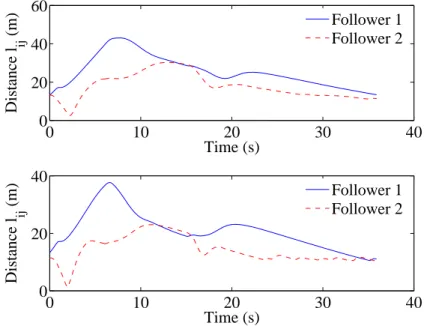
3.19 13 robot formation. Top: Desired formation configurations, G1 if t≤ 11s, G1 if t > 11s. Bottom: trajectories . . . 40
3.20 Trajectory generation convergence. . . 42
3.21 Formation desired velocities. . . 43
3.22 Leader-Follower formation configuration. . . 44
3.23 Circular xdf oll trajectory. . . 46
3.24 Leader-Follower stabilization with saturated follower velocity, for a constant circular leader trajectory.G = {1},{(0,1)},l01 = 10m, γ01 = π /4rad. . . 48
3.25 Leader-Follower relative distance ll− f and angle γl− f, for a constant circular leader trajectory . . . 49
3.26 Leader-Follower stabilization for a transient leader maneuvering with saturated follower velocity. . . 49
3.27 Robot trajectories. G = {1,2},{(0,1),(0,2)}, l01d = l12d = 20m, γ01d = γ12d = π/4rad, v0= 5m/s, ξ0= π/90rad vmax1= vmax2= 12.5m/s . . . 50
3.28 Relative leader-follower distances and angles. Stationary leader tra-jectory example. G = {1,2},{(0,1),(1,2)}, l01d = l12d = 20m, γ01d = γ12d = π/4rad, v0= 5m/s, ξ0= π/90rad, vmax1= vmax2= 12.5m/s . . 51
3.29 Robot trajectories. G = {1,2,3},{(0,1),(1,2),(2,3)}, l01d = l12d = l23d = 20m, γ01d = γ12d = π/4rad, γ23d = πrad, v0= 5m/s, ξ0= π/90rad, vmax1= vmax2= vmax312.5m/s . . . 52
3.30 Relative leader-follower distances and angles. Stationary leader tra-jectory example. G = {1,2,3},{(0,1),(1,2),(2,3)}, l01d = l12d = l23d = 20m, γ01d = γ12d = π/4rad, γ23d = πrad, v0= 5m/s, ξ0= π/90rad, vmax1= vmax2= vmax312.5m/s . . . 53
3.31 Robot trajectories. Non stationary leader trajectory example. G = {1, 2}, {(0, 1), (1, 2)},ld 01= l12d = l23d 20m, γ01d = γ12d = π/4rad, v0= 12.5m/s, vmax1= vmax2= 15m/s . . . 53
3.32 Relative leader-Follower distances and angles. Non stationary leader trajectory example trajectory. G = {1,2},{(0,1),(1,2)},ld01= l12d = l23d 20m, γ01d = γ12d = π/4rad, v0= 12.5m/s, vmax1= vmax2= 15m/s. . . 54
4.1 Deformable virtual zone definition . . . 56
4.2 Undeformed DVZ . . . 56
4.3 Total DVZ deformation Jobst(t) . . . 58
4.4 Robot’s ultrasonic sensors . . . 58
4.6 Robot’s trajectories. Formation: V = {1,2} with the leader robot
0. Nodes E = {(0,1),(0,2)}. Desired relative positions l01 = l02 =
10m,γ01= −γ02= π4. Bounded computing time Ts= 300ms . . . 60
4.7 Up: robots velocities, down: robot’s steering angle. Formation: V = {1,2} with the leader robot 1. Nodes E = {(0,1),(0,2)}. De-sired relative positions l01 = l02 = 10m,γ01 = −γ02 = π4. Bounded computing time Ts= 300ms . . . 61
4.8 Trajectory generation simulation: unbounded time condition. (a) Trajectory. (b) Iterations number . . . 61
4.9 Trajectory generation simulation: bounded time condition. (a) Tra-jectory. (b) Iterations number . . . 62
5.1 Multipath effects on a mobile station . . . 65
5.2 RSS location estimation . . . 66
5.3 Identification of RSS propagation model. Experimental setup . . . . 67
5.4 Results for identification of RSS path-loss model . . . 67
5.5 Position estimation. . . 70
5.6 Distance estimation. Circular trajectory example . . . 70
5.7 Distance error. Circular trajectory example . . . 71
5.8 Position trajectory estimation. G = {{1,2},(0,1),(1,2)},l01= l12 = 100m, γ01= γ12= π/4. We suppose that the RSS is measured between the nodes (0,1) and (1,2) . . . 71
5.9 Leader-Follower-1 RSS estimation . . . 72
5.10 Leader-Follower-1 relative angle γ . . . 72
5.11 Leader-Follower-1 distance estimation error . . . 73
5.12 Experimental setup . . . 73
5.13 RSS estimation . . . 74
5.14 Distance estimation . . . 74
6.1 Trajectory tracking problem . . . 75
6.2 Trajectory generation and tracking. . . 76
6.3 Linearized system, non-controllable condition. γd= ±π/2 and (γd= 0, ξd= 0) . . . 80
6.4 Closed-loop relative distance li j. . . 80
6.5 Closed-loop relative angle γi j. . . 81
6.6 Closed-loop linear velocity vj. . . 82
6.7 Closed-loop steering angular velocity ωj. . . 82
8.1 Flottille de robots mobiles . . . 87
8.2 Strat´egie de commande d´ecentralis´ee . . . 88
8.3 (a) Delta, (b) Lin´eal . . . 88
8.4 Positionnement Leader-Follower . . . 89
8.5 D´efinition de la trajectoire optimale . . . 90
8.6 Algorithme de g´en´eration de trajectoires en temps r´eel. . . 91
8.7 Flotille: V = {1,2}, E = {(0,1),(0,2)}. l01= l02= 10m,γ01= −γ02= π 4. Gauche τ = 300ms. Droite τ = 500ms . . . 92
8.8 Distance relatif li j: V = {1,2}. E = {(0,1),(0,2)}. l01 = l02 = 10m,γ01= −γ02= π4. En haut τ = 300ms. En bas τ = 500ms . . . 92 8.9 Angle relatif γi j: V = {1,2}. E = {(0,1),(0,2)}. l01= l02= 10m,γ01= −γ02= π4. En haut τ = 300ms. En bas τ = 500ms . . . 93 8.10 Vitesse vi: V = {1,2}. E = {(0,1),(0,2)}. l01 = l02 = 10m,γ01 = −γ02= π4. Gauche τ = 300ms. Droite τ = 500ms . . . 93 8.11 Angle de braquage ξi: V = {1,2}. E = {(0,1),(0,2)}. l01 = l02 = 10m,γ01= −γ02= π4. Gauche τ = 300ms. Droite τ = 500ms . . . 94
8.12 Flotille 13 v´ehicules. En haut foltilles d´esir´ees, G1 si t ≤ 11s, G1 si
t> 11s. En bas, trajectoires . . . 94
8.13 Zone virtuelle d´eformable . . . 95
8.14 Evitement d’obstacles. Formation: V = {1,2}, E = {(0,1),(0,2)}.
l01= l02= 10m,γ01= −γ02 =π4. Ts= 300ms . . . 95
8.15 Identification du model de propagation. Exp´erimentation . . . 96
8.16 Estimation de position pour un robot en utilisant le niveau de r´
Introduction
Over the past several centuries, progress in sparing humans from hard labour has accelerated. Throughout the world, animals and machines now perform many work activities, providing many with easier lives, greater safety and more indepen-dence. The drive to find substitutes for humans in hazardous environments and fatiguing activities has been one of the principal motivations for the search for autonomous and secure systems. The Egyptian, Roman and Greek civilizations took advantage of the more developed sensors of dogs and domesticated them for use in exploration and hunting. Over time, even more autonomous solutions were found with the introduction of various mechanical innovations. The Greeks used their understanding of hydraulic principles to operate statues that imitated human characteristics. In 12th century China, a south-pointing chariot was equipped with a statue that was turned by a gearing mechanism attached to the chariot wheels in such a way that it continuously pointed south. Hence, using the directional information provided by the statue, the charioteer could steer a straight course. In more recent times, such mechanical innovations have been combined with progress in computing power and theoretical and technological advances, giving rise to the field the robotics. Robotics as it is known today is a vast interdisciplinary science comprising many fields of research, including vision, sensing, dynamics, motion planning and control, locomotion, and design. One of the most basic problems, however, remains the motion planning and control of robots. Robot motion plan-ning deals with finding a feasible trajectory for a robot moving in an environment with obstacles.
Since a single robot, no matter how capable, is spatially limited, the study of multi-robot systems has became a major focus in the robotics research community. Although the field of multiple robot systems naturally extends the research on single robot systems, it is also a discipline in itself: multiple robot systems can accomplish tasks that single robots cannot. Multi-robot systems are also different from other distributed systems because of the implicit real-world environment.
The study of multi-robot systems entails the analysis of cooperation and coor-dination laws between the robots. Cooperation in multi-robot systems was defined by Farinelli et al [1] as the ability of a system to cooperate in order to accomplish a specific task; coordination was defined as the set of mechanisms and interactions used to obtain this cooperation. In chapter 2, we review and extend these concepts.
Coordination in a multi-robot system can be achieved by means of explicit com-munication between robots via sonar for underwater and terrestrial robot systems and radio communication for aerial systems.
Coordination by means of explicit communication allows the robot formation to be spread over a much wider area compared with other coordination mechanisms like vision. One of the chief concerns in real-world applications of multi-robot systems is security, designed as the ability of the individual robots to continue interacting with the other robots while they perform a predefined team task. To ensure this coordination between robots, the communication also has to be carried out in some autonomous way by the set of robots.
As it will be discussed, the aim of this thesis is to investigate motion planning in nonholonomic multi-robot cooperative systems. We were motivated by applications in unstructured environments, especially for the performance of outdoor tasks like rescue, surveillance and exploring. The multi-robot system is subject to many constraints like, such as obstacles in the environment, many possible paths for each robot, the avoidance of communication losses, and the many ways in which the robots can be organized in the formation. For this reason, the optimal solution might be a highly decentralized path planning procedure for this type of system. In this approach, for example, the communication variables are taken into account to ensure the interaction of the robots while the task of the formation is being accomplished in the unstructured environment.
1.1 Approach
Many approaches to planning and controlling the trajectory of nonholonomic mobile robots have been described in the literature and will be presented in chapter 2. Trajectory planning can be classified as either online or offline. The online methods use knowledge of the current system state and its environment to plan the motion for the next time instant. Since these strategies do not require any pre-computation, they are suitable for tasks that do not require any specific constraints to be satisfied along the trajectory, i.e. for tasks whose only requirement is the desired goal configuration. Such schemes are rarely concerned with finding and optimizing a feasible trajectory. On the other hand, the offline approaches rely on prior information about the desired task and the environment configuration, taking into account the systems constraints. Consequently, a feasible open-loop trajectory can be found and optimized.
In multi-robot systems control, the trajectory planning of each nonholonomic robot also depends on the desired cooperation between the robots, i.e. the deci-sion about whether a predefined geometrical pattern is needed between the robots. The robots can be coordinated in a centralized or decentralized way to achieve the desired tasks. In a centralized organization, the trajectory planning relies on information about all the robot positions and there is thus a central trajectory com-puting agent. In contrast, decentralized coordination uses only local information for each robot. Therefore, no central computing agent is required.
In the following work, a new secure control strategy for multiple car-like vehicle formation is proposed. Distributed trajectory planning is used to obtain an
open-loop trajectory for each robot in the formation. The desired trajectory for each robot is a locally optimal solution; in this optimization problem a reactive term is incorporated for the obstacle avoidance constraint in unknown environments. We also incorporate vehicle and trajectory constraints, such as a saturation of the controls and the desired position in the formation for each robot.
In real applications of multi-robot systems, security is a major consideration in the design of the control strategy. For instance, to ensure that the breakdown of a single mobile robot does not jeopardize the mission of the whole formation, the required communication between robots has to be maintained and the data (i.e. position) measurement has to be guaranteed. We propose the use of a global positioning system (GPS) for the position measurement and a WiFi network as the communication platform. For this purpose, the communication link between robots is secured by measuring the WiFi reception signal of each robot and incorporating it into the trajectory generation scheme.
1.2 Problem Definition
The aim of this thesis is to study the control of cooperative terrestrial non-holonomic autonomous vehicles, which can be formulated as follows: Given: the instantaneous position and orientation of a leader agent and the initial positions of a set of n robots in the workspace generate a continuous trajectory for each robot, with each robot avoiding obstacles, keeping a predetermined geometrical pattern with respect to the leader agent, and being subject to the dynamical constraints of vehicles. We elaborate a decentralized trajectory generator that computes a feasible trajectory for each robot in the formation while respecting the dynamical constraints of vehicles and the desired geometrical pattern of the formation. In addition, we prove the stability of this approach through simulations and experi-ments.
1.3 Contribution
In this thesis, we develop two specific contributions to the control of multi-robot systems, which can be summarized as follows:
• First, we develop a general, highly decentralized strategy to control forma-tions of cooperative nonholonomic robots. Under this strategy, the highlights of online and offline path-planning techniques are summarized in a single con-trol approach of nonholonomic cooperative robots. A feasible trajectory is computed for each robot; if any obstacle is detected, the trajectory is modified using a defined reactive term. Then the stability condition of the strategy for a formation of n robots is also shown. This trajectory generation process is based on an optimization problem for which several optimization criteria can be included, i.e. minimal communication link losses or minimal time trajectories or composites of them.
• Second, we propose an approach using the reception signal strength (RSS) of the wireless communication to secure the communication links between
robots. By measuring the reception signal of the wireless communication architecture, we develop a strategy to guarantee these communication links. Also, the use of the RSS is proposed as an alternative relative-positioning mechanism for the robots when the classical positioning systems like GPS are unavailable.
1.4 Thesis Outline
Chapter 2 presents the previous work in mutli-robot system control and non-holonomic path-planning fields. In the first part, the approaches to control multi-robot systems are presented, as well as the online and offline methods for the path planning and control of nonholonomic robots, such as trajectory optimization problems and reactive methods for obstacle avoidance. In chapter 3, we develop a general mathematical model for decentralized control of nonholonomic robot forma-tions, including dynamical constraints in the framework of the calculus of variations to achieve an optimal solution. A numerical method is then proposed to obtain feasible, fast and accurate solutions. Also in this chapter is formulated the sta-bility conditions for the proposed strategy. For a geometrical formation of robots, each robot is subject to different desired orientation velocities, depending on its position in the formation. For example, for the rotation of a delta formation, the farthest vehicle with respect to the instantaneous centre of rotation of the desired formation pattern can be subject to higher velocities than the maximal admissible vehicle velocity. We develop the constraints in manoeuvring the desired formation to keep the robot formation by inserting these constraint equations in the computa-tion of the agent leader’s trajectory. Last, we present our study of the transit-time performance of the proposed strategy.
In Chapter 4, a obstacle avoidance approach is proposed. We define a reactive term which is to be included into the trajectory generator. This reactive term is based on a Deformable Virtual Zone (DVZ) [4] that surrounds each vehicle. By computing the virtual zone deformation caused by the obstacles the trajectory gen-erator search a path that minimizes this deformation. Hence the feasible trajectory is adapted for obstacle avoidance.
Chapter 5 includes the estimation of the reception signal level of the wire-less communication system into the decentralized trajectory generator in order to maintain the communication link between robots. By using the signal level we can estimate the leader-follower relative position if the global positioning system (i.e GPS) is no available.
In Chapter 6, a feedback controller is proposed for the leader-follower model. The robot is stabilized about the reference path by defining a linear quadratic regulator (LQR). The controlled variables is the relative leader-follower position. Finally in chapter 7, the final remarks and the proposed future works are detailed.
State of the Art
In this chapter, we survey the state of the art in nonholonomic multi-robot systems. We first describe and contrast the studies on different multi-robot control strategies. Then, we present the principal approaches for nonholonomic mobile robot control. In particular, we focus on trajectory planning, as well as the sta-bilization procedures for the car-like robots. Last, advances in the robotics field are highlighted with special attention to positioning and communication systems as applied to robotics.
2.1 Cooperative Multi-Robot Systems
Multi-robot systems are currently a major focus of research in the field of robotics. Multi-robot systems can accomplish tasks that a single robot cannot, since a single robot will ultimately be spatially limited. In 1989, Brooks and Flynn from MIT’s Artificial Intelligence Lab proposed what they called a radical idea in the solar system exploration field: replace a large rover by a collection of small rovers [5]. They said that the cost per kilogram of the rovers would be greatly reduced from the economy of building multiple copies. Lower reliability for each in-dividual rover would be acceptable, as failure of a single rover would not jeopardize the whole mission. Indeed the mission could be planned with a particular reliability expectation that was below 100%. Upon landing either together or in smaller groups, the rovers would disperse covering wide ranges over the surface. This radical idea presents the main motivation for the use of multi-agent robotic systems.
Among the first studies on multi-robot systems were those of Fukuda (cellular robotics [6]), and other MIT researchers working in the field of robotic societies of up to twenty mobile robots: [7], [8]. Other pioneering efforts in multi-robot systems study came from Stanford [9], and Carnegie Mellon [10], universities.
More recently, multiple autonomous mobile robots have been proposed for use in rescue missions [11], [12], exploration [13],[14], [15], military applications, and even entertainment with robotic soccer teams [16],[17].
A multi-robot system can be defined as a set of robots operating in the same work space [1]. In addition, cooperative behaviour is settled as: Given some task specified by a designer, a multiple-robot system displays cooperative behavior if, due to some underlying mechanism (i.e., the mechanism of cooperation or coordination), there
is an increase in the total utility of the system. [18].
In the following sections, we present the principal features of cooperative multi-robot systems. We discuss the main works in this field, with special attention given to the formation of nonholonomic robots.
2.1.1 Multi-Robot Systems Classification
Given the variety of designs of multi-robot systems, it is useful to have them organized. [19], [18],[1], developed the taxonomy of these systems. Farinelli’s [1] classification relies on the coordinative nature of the robot set. This taxonomy is represented by the hierarchical structure shown by Figure 2.1.
At the cooperative level, we can distinguish cooperative systems from non-cooperative ones. A non-cooperative system is composed of robots that operate together to perform some global task. Farinelli’s work, also considers the coordinative level. Coordination is a cooperation in which the actions performed by each robotic agent takes into account the actions executed by the other robotic agents in such a way that the whole ends up being a coherent and high-performance operation. Orga-nization level introduces a distinction in the forms of coordination, distinguishing centralized approaches from distributed ones. In particular, a centralized system has an agent (leader) that is in charge of organizing the work of the other agents; the leader is involved in the decision process for the whole team, while the other mem-bers can act only according to the leader’s directions. In contrast, a distributed system is composed of agents that are completely autonomous in the decision pro-cess with respect to each other; there is no leader in such cases. The classification of centralized systems can be further refined depending on the way the leadership of the group is played. Specifically, strong centralization is used to characterize a system in which decisions are taken by the same predefined leader agent through-out the entire mission, while in a weakly centralized system more than one agent is able to take the role of the leader during the mission.
Instead of a classification based on coordination as proposed by Farinelli et al; the classification of Cao et al. [18] relies on the structure of the robot set. According to this classification, a multi-robot system can be homogeneous or heterogeneous. A group of robots is said to be homogeneous if the capabilities of the individual robots are identical, and heterogeneous otherwise. Then, the centralized or decentralized
architecture is described. Similar to Farinelli’s description, Cao et al. defined centralized multi-robot systems as formations characterized by a single control agent. A decentralized organization lacks such an agent. They included two types of decentralized organizations: distributed architectures in which all agents are equal with respect to control, and hierarchical architectures which are locally centralized. In addition, hybrid centralized/decentralized architectures are also described. In these architectures, there is a central planner that exerts high-level control over mostly autonomous agents. A hybrid control architecture for autonomous robot platoons was presented by [20]. In this strategy each robot executes its control locally but relies on the state of all robot set.
One of the main objects of study in multi-robot systems research is the munication or interaction between the robots. [18], [19], studied the different com-munication structures in these systems. The comcom-munication structure of a group determines the possible modes of inter-agent interaction. Three main structures are discussed in these works. First is communication or interaction via environment: this occurs when the environment itself is the communication medium, and there is no explicit communication between agents. This type of interaction between robots is also known as stigmergy and examples can be found in [21]. Another typical structure is the interaction via sensing: this refers to local interactions that occur between agents as a result of them sensing one another, but without explicit communication. An example would be vision by means of omnidirectional cameras [22]. Last is interaction via communications: this involves explicit communication with other agents, by either directed or broadcast intentional messages. Because architectures that enable this form of communication are similar to those of commu-nication networks, many standard issues from the field of networks arise, including the design of network topologies and communications protocols.
2.2 Nonholonomic Systems
Mobile robots are useful for transport, inspection and intervention in hostile environments. Therefore, the use of mobile robots agents for multi-robot systems applications is becoming increasingly prevalent in academics, military and indus-trial sectors because their efficiency and flexibility.
The motion of a wheeled mobile robot is subject to nonholonomic constraints due to the rolling constraints of the wheels, which make a motion perpendicular to the wheels impossible. Because of these nonholonomic constraints, the implemen-tation of multi mobile robots is a challenging problem for the multi-agent theory, as well as for the nonlinear control theory.
The analysis and study of multi-robot systems differs from that of multi-agent systems because of the issues arising when dealing with a physical environment, such as uncertainty and the incompleteness of the information acquired from the environment. In fact, the need to cope with the acquisition of knowledge from a real environment makes the experimental evaluation of multi-robot systems much more challenging. In addition, the forms of cooperation used in multi-robot systems need to take into account the uncertainty, limitations, and mistakes arising from the processing of sensor information.
Nonholonomic multi-robot system naturally extend the problems of studying a single nonholonomic autonomous vehicle. Consequently, an examination of the latest research efforts in autonomous multi-agent systems and the control of non-holonomic mobile robots is called for.
2.2.1 Control of Nonholonomic Systems
The word holonomic (or holonomous) is comprised of the Greek words meaning integral and law, and refers to the fact that such constraints, given as constraints on the velocity, may be integrated and reexpressed as constraints on the config-uration variables [23]. Examples of holonomic constraints are length constraints for simple pendula and rigidity constraints for rigid body motion. In contrast, nonhonolonomic mechanics describes the motion for systems with nonintegrable constraints; for example, constraints on the system velocities that do not arise from the configurations alone. Classic examples are rolling and skating motions.
The principal characteristics of nonholonomic mechanical systems can be illus-trated by the unicycle system example (Fig. 2.2).
Fig. 2.2: Unicycle system
The kinematic representation of the unicycle system with steering speed ˙θ = u1
and rolling speed v = u2 as controls can be modelled by the equation:
˙ x= u2cos(θ ) ˙ y= u2sin(θ ) (2.1) ˙ θ = u1, with the nonholonomic constraint:
˙
ycos(θ ) − ˙xsin(θ ) = 0, (2.2)
Therefore, the allowed velocities (u1, u2) have to get into the null space of the
restriction matrix a(q), with q = [x, y, θ ]:
aT(q) = [sin θ − cos θ 0] ⇒N (a(q)) = span
cos θ sin θ 0 , 0 0 1 .(2.3)
The condition (2.3) implies that for each configuration q there is only two possible
field of the rolling forward movement of the unicycle at unit velocity, and g2=
[ 0 0 1 ]T, its spinning counterclockwise at unit velocity. Hence, the unicycle
capacity of rolling forward and backward and spinning in place can be represented
by the vectors fields g1, g2. The graphical representation of vector fields for the
unicycle example can be seen in the Figure (2.3).
Fig. 2.3: Unicycle’s vectorial champ. q1, q2 manoeuvring
This restriction over the possible state evolutions in nonholonomic systems has to be taken into account in the design of the control strategy.
In the literature, two main strategies to control wheeled mobile robot control systems have been described: open-loop and closed-loop (feedback).
The open-loop strategies seek feasible trajectories in the free configuration space that connect an initial configuration with a final one. They take into consideration several criteria like collision-avoidance, the shortest path, and minimum control effort. The shortest path with a lower bound on its radius between two oriented points in the plane was studied by Dubins [24]. Such as path is composed of at most three segments of straight lines and arcs. In this case, according to Reeds and Shepp [25], more manoeuvrability is added to the shortest path by using at most five segments of arcs and straight lines. Laumond [26] proposed an algorithm for planning manoeuvres and collision-free paths for circular nonholonomic robots whose turning radius was lower bounded. These open-loop techniques do not com-pensate for disturbance, system model errors or changing configuration space.
In the closed-loop procedures, the input is a function of the state to compensate for errors and disturbances. Generally, there is no smooth feedback control law that makes a given configuration asymptotically stable. This means that the class of stabilizing controllers should be suitably enlarged so as to include nonsmooth
and/or time-varying feedback control laws (i.e [27]). This is a consequence of
Brockett’s theorem [28], and was also discussed in [29] and has also been discussed in [23]. Given the lack of smooth state feedback laws, works on path following and tracking rely on non-zero reference motion. A survey of local tracking problems for a cart was presented [30]. Ailon et al. [31] presented a controllability study of the trajectory tracking problem of a front-wheel drive car-like vehicle. Other control strategies have been used for local tracking control of wheeled vehicles, such as PID controls [32] or sliding mode [33], [34], for example.
By reason of the assumption of non-zero reference motion, stabilization about a fixed configuration cannot be treated by these tracking approaches. Consequently, since there is no smooth control law that stabilizes wheeled mobile robots about a fixed configuration, other classes of feedback strategies have been considered, i.e. discontinuous and time-varying control laws. Nonsmooth controls have been proposed to stabilize nonholonomic vehicles [35],[29], [36],[37].
For open-loop and closed-loop strategies with non-zero reference motion, a fea-sible trajectory is required. Motion planning for nonholonomic systems has been the subject of a great deal of recent research. The motion planning problem for nonholonomic vehicles can be classified by the nature of the problem, i.e. with or without obstacles or cost function to be minimized. Among the first approaches to mobile robot motion planning were the Dubin’s [24], and Reeds & Shepp’s [25], works. In both approaches a minimal length solution is obtained for robots in obstacle-free spaces. Also, techniques of non linear optimization can be applied (i.e. [38]). Using these approaches, the control history or trajectory is finitely parameterized. The differential flatness property [39], of certain nonholonomic systems, like the car-like vehicle, has been applied to the optimization strategies; for example, in Van Nieuwstadt’s [40], and Milam’s [41], trajectory generation al-gorithms. Using the flatness property of the vehicle system, the problem dimension was reduced and more computation efficiency was obtained.
2.3 Motion Coordination
The study of motion coordination of nonholonomic robot formations extends the study of motion planning of single robot. Motion coordination is a remark-able phenomenon in biological systems and an extremely useful tool for groups of vehicles. These coordination tasks must often be achieved with minimal commu-nication between the agents and also limited information about the global state of the system. The application of these biological inspired coordination strategies should take into account the local properties of the agents, like controllability and other constraints like saturation of states and controls. Many decentralized multi-robot motion coordination research works are based in the motion of particles or the simplified models of the robot agents. In other hand, the coordination strate-gies which take into account the nonholonomic robot constraints often need the information of the global state of the system. We present some general strategies and analysis tools for multi-robot motion coordination, and specific applications to nonholonomic formations.
2.3.1 Artificial Potentials
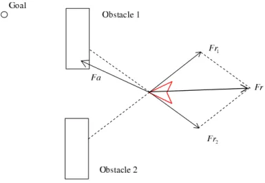
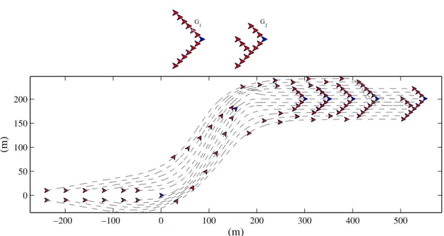
Leonard and Fiorelli [42], proposed the artificial potentials which define inter-action control forces between neighboring vehicles and are designed to enforce a desired inter-vehicle spacing. A virtual leader is used to influence in its neighbor-hood by means of additional artificial potential, then the virtual leader is used to manipulate group geometry and direct the motion of the group. This framework can be applied to homogeneous groups with no ordering of vehicles, Ozdemir and
Temeltas [2], define a turning rule of the potential forces to avoid the local mini-mum problems. The main drawback of these approaches, is that they are based on point mass agents and no physical or dynamical constraints are included into the model. The forces over a agent are shown in Figure 2.4
Fig. 2.4: Ozdemir and Temeltas [2], artificial potential method. Obstacle, virtual leader and modified obstacle forces definition.
2.3.2 Leader-Follower
The Leader-follower strategy was first introduced in control system by the Ger-man economist Heinrich Freiherr von Stackelberg who published Marktform und Gleichgewicht in 1934 which described this model (see [43]). These control method-ologies, also known as Stackelberg strategies, are appropriate for classes of system problems where there are multiple criteria, multiple decision makers and decen-tralized information. In these strategies, the follower control actions are based on the leader’s state and control. The leader-follower concept has been widely used in multi-robot control. Feddema et al [44], studied the observability and reachability of leader-follower based control of cooperative mobile robots. Other leader-follower applications in multi-robot systems have been presented for terrestrial vehicles
” [45], [22], [46], aerial autonomous multi-robot systems [47],[48] and unmanned un-derwater vehicle platoons [49],[50].
In the leader-follower approaches, each robot agent is positioned in the for-mation by the relative geometry with respect to its predefined neighbour. Each robot follows its predefined leader with a certain geometrical relationship. Using this leader-follower relationship, a geometrical pattern of n robots can be obtained. Typically, there is a single leader of the formation. This single leader does not fol-low any other robot in the set, but a predefined trajectory. The stability of leader-follower-based multi-unicycle robot systems was studied by Lechevin et al., [51]. The stabilization was proposed for a formation of unicycles where the relative angle between the robots remained constant in time. Also using the leader-follower ap-proach, Desai et al. [52], proposed a stabilization strategy of multiple autonomous nonholonomic robots. A framework based on graph theory for transitioning from
one geometrical pattern to another was presented. Among the applications of the leader-follower strategies, the work of Dasset al. [22]: proposed vision-based stabi-lization of the formation of car-like vehicles.
2.3.3 Centralized Motion Planning
Another point of view in motion planning for multi-robot systems are the cen-tralized planning strategies. In general, a reference trajectory is defined for the platoon then the single robot paths are computed with respect to this reference trajectory. Such of use of a reference point for all robots this strategy can be con-sidered as a centralized approach, all robots should be able to know their distance to this reference point.
Among this strategy, Barfoot and Clark [3], propose a planning approach for mobile robot in formation, as formation they refer to certain geometrical constraints which are imposed on the relative positions and orientations of the robots through-out their travel. For platoons of nonholonomic robots keep the geometrical pattern for some manoeuvering is not possible, such of that the Barfoot and Clark work proposed to control the formation in a curvilinear coordinates rather than in the original rectilinear coordinate system. This takes advantage of the non-holonomic constraint imposed on each robot. It also ensures that for a static formation which does not turn sharper than a threshold curvature, the individual robot trajectories will not collide. They introduce an arbitrary reference point, within the formation whose coordinates serve as a single set of reference coordinates for the group. This point could be the center of the formation, one of the robots in the formation, or any other point. All robots in the formation will be described relative to this reference point (but in curved space).
Fig. 2.5: Square and turning square formation. In curvilinear coordinates. KC, Ki are the
curvature coefficients for the reference C and robot i points. Barfoot and Clark [3]
2.3.4 Redundant Manipulator Techniques
The redundant manipulator approaches [53] have been applied by the Stilwell’s [20], and Bishop’s [54] works to stabilize formations of nonholonomic robots. These works were based in semi-decentralized structures. Each autonomous vehicle com-putes its trajectory using an exogenous feedback signal. This method was applied to formation of autonomous underwater robotic formations [55]. This strategy, to controlling a platoon of vehicles was based on the concept of controlling the platoon,
not the individual vehicles. While the global behavior of the platoon is regulated, the individual vehicles behaviors are not. Indeed, the local behavior of each vehicle is not known until the closed-loop system is simulated. The goal of this approach is to regulate the platoon, thus, a suitable measure of the platoon performance is required. Any function of the platoon that can be exogenously measured will suffice. Such functions are referred to as platoon functions. In short, the Stillwel’s strategy proposes a set of decentralized controllers that are implemented on each vehicle and an exogenous system that broadcasts information to the platoon, hence the approach is called semi decentralized.
They consider the the average position of the vehicles in the plane and the distribution of the vehicle positions about the average, as specific platoon functions throughout for the purposes of illustration and motivation. Overall, the control goal is to stabilize the formation about a reference trajectory of the platoon functions by controlling each vehicle velocity. As for a platoon function it can be a large number of robot configuration, the techniques of redundant manipulators are a useful stabilization strategy.
2.4 Collision-free Motion of Robots
An important task of motion planner is the navigation or the problem of finding a collision-free motion for the robot system from one configuration to another. There exists many navigation algorithms that can solve this problem. Like optimal or non-optimal solutions, online or off-line, sensor-based or world model based, etc. Optimal solutions search motions that are optimal in some way, such as distance, time, or energy. The computational complexity often depends on the memory requirements and running time of the algorithm, finally we say a planner is off-line if it constructs the plan in advance, based on know model of the environment, contrary, an online algorithm incrementally constructs the plan while the robot is executing the tasks.
2.4.1 Reactive Control
Reactive control is a term we use to describe a wide variety of schemes that have been proposed to enable robots to move without collision. Although the term is vague, what these schemes have in common is a philosophy of determining the desired motion of the robot in real time by examining some up-to-date model of the world. As the model of the world changes, the robot reacts. Typically, the model of the world is determined by the robot sensors. Also, the model may be local in that it is a function only of the current sensor information and does not contain global state that is determined over time. Reactive control goes under many names such as reactive behaviors, behavior-based control, sensor-based control, and local collision avoidance. In the following, three reactive control schemes are described: boundary following, potential fields and deformable virtual zones.
2.4.1.1 Boundary Following
The Bug1 and Bug2 algorithms [56], are among the simplest sensor-based path planning approaches. These algorithms assume the robot is a point operating in the plane with with a sensor to detect obstacles. The Bug algorithms formalizes the idea of moving toward the goal and going around obstacles. Perhaps the most straight forward path planning method is to move toward the goal, unless an obstacle is encountered, in which case, circumnavigate the obstacle until motion toward the goal is once again allowable. In Bug1 algorithm, the robot drives straight to the
goal, if the robot encounters an ith obstacle, let qHi be the hit point; the robot
then circumnavigate the ith obstacle and determines the closest point to the goal,
this point is called the leaving point (qLi), from (qLi) point the robot drives direct
to the goal point, and reinvokes the last described behavior. The Bug2 algorithm
determines the leaving points (qLi) by searching the interception of a straight line
from the start point to the goal. Then, if the robot encounters any obstacle it follow the obstacle until the leaving point. The Figure (2.6) shows sketch the Bug algorithm behavior.
Fig. 2.6: Bug1 (up) and Bug2 (down) algorithms
Other variation of the Bug algorithm is the Tangent Bug algorithm [57], specifi-cally designed for using a range sensor with a 360 degree infinite orientation resolu-tion. These Bug algorithms are applicable only to two Degree Of Freedom (2-DOF), robots.
2.4.1.2 Potential Functions
For some motion planning problems explicitly representation of the configura-tion space can be difficult, such of that,an alternative is to develop search
algo-rithms that incrementally explore free space while searching for a path. The Bug algorithms can be used for this task, but they are limited to two-dimensional con-figuration spaces. The artificial potential function method can produce a greater variety of paths than the Bug methods, and can be applied to more general class of configuration spaces, this method is based in artificial forces acting on the robot. The idea of imaginary forces acting on a robot has been suggested in 1983 by An-drews and Hogan [58] and in 1985 by Khatib [59]. In these approaches obstacles exert repulsive forces onto the robot, while the target applies an attractive force to the robot. The sum of all forces, the resultant force, determines the subsequent direction and speed of travel.
A potential field function is a differentiable real function U : Rm→ R. The value
of this potential function can be interpreted as energy and hence the gradient of
the potential is force. Then the gradient is a vector 5U (q) = [∂U
∂ q1, ...
∂U ∂ qm]
T, this gradient points in the direction that locally maximally increases U . The potential function approach directs a robot as if it were a particle moving in a gradient vector field. Gradients are artificial forces acting on a positively charged particle robot which is attracted to the negatively charged goal.Obstacles have a positive charge which form a repulsive force directing the robot away from obstacles. Therefore combining the repulsive an attractive forces directs the robot from a start position to the goal while avoiding obstacles. The resulting force makes the robot follows a path descent or so called downhill path by following the negated gradient of the potential function. Following such a path is called gradient descent, i.e.:
˙q = − 5U (q)
Then the problem is to define additive attractive and repulsive functions, usu-ally defined as function of the distance to the goal for the attractive forces and to the obstacles for the repulsive ones.
Koren and Borenstein [60], studied the main drawbacks of the artificial poten-tial field methods. Among this drawbacks they cited:
Local minima or trap-situations. Perhaps the best-known and most often-cited problem with potential field methods is the problem of local minima or trap-situations. A trap-situation may occur when the robot runs into a dead end, for example a U-shaped obstacle.
No passage between closely spaced obstacles, for a closely space the repulsive forces on the robot can be pointed away from the space (see Fig. 2.8).
Also, Koren and Borenstein described oscillation conditions in narrow corridors and for the presence of large obstacles.
2.4.1.3 Deformable Virtual Zone
Although this formalism has been highly used in mobile robotics, the nonholon-omy of most of them complicates the use of it. The induced kinematic constraints
Fig. 2.7: Local minima condition in potential field methods
Fig. 2.8: For the potential field method the robot does not pass between closely spaced obstacles
may not allow the robot to execute instantaneously every motion, which may be lead an avoidance task to end in failure. This issue is addressed by Zapata et al with the DVZ approach (Deformable Virtual Zone) [4]. This consists in surround-ing the robot with a virtual zone which can be deformed dependsurround-ing on two modes. The first one is called controlled mode. The shape of the zone is modified according to the internal state of the robot. The second mode is the uncontrolled mode of deformation. When an obstacle tries to come into the zone, it deforms its shape, as it was made of a supple membrane. The controls are computed in order to minimize this uncontrolled deformation.
2.4.2 Planning and Reactive Control
When building a robot system, we ideally would like to combine both path plan-ning and reactive control. Path planplan-ning provides the ability to move to specified goal positions, even in the presence of complex obstacles. Reactive control provides robust performance in order to deal with uncertainties and unexpected obstacles while executing the planned path. Hence, we can say that this two concepts are excluding definitions. If we have an ideal or perfect planning solution, it will be not necessary any reaction of the system. However, to perform an ideal planning, we require to have all the information about the environment like obstacles, trajec-tories of moving objects etc. In real applications of robotic system, only a reduced
information if often available, then an adaptive planning or combining planning and reactive control is desirable approach for some robotic application. One com-mon approach to combining planning and reaction involves replacing paths as the specification of the planned motion of a robot. By designing a representation that reduces the level of commitment inherent in a path, a reactive controller can adapt the motion of the robot in response to information obtained during execution while still following the original plan
Some works address the adaptive planning strategies. Quinlan [61], propose a real time modification of robot collision-free paths. This method uses the elastic bands approach [62], to planning the robot path, then this trajectory is modified by the sensor information in real-tme, the strategy was validated in a PUMA 560 manipulators.
In 2004 Lamiraux et al [63], propose a generic approach of path optimization for nonholonomic systems. This approach is applied to the problem of reactive navigation for nonholonomic mobile robots in obstacle environments. This is a collision-free initial path being given for a robot, and obstacles detected while following this path can make it in collision. The current path is iteratively deformed in order to get away from obstacles and satisfy the nonholonomic constraints, they use the potential field method to deform the initial trajectory based on the real-time sensor information.
2.5 Localization
In general, the methods for locating mobile robots in the real world are di-vided into two categories: relative positioning and absolute positioning. In relative positioning, odometry and inertial navigation (gyros and accelerometers) are com-monly used to calculate the robot positions from a starting reference point at a high updating rate. Odometry is one of the most popular internal sensor for position estimation because of its ease of use in real time. In contrast, the disadvantage of odometry and inertial navigation is that it has an unbounded accumulation of errors, and the mobile robot becomes lost easily. Consequently, frequent correction based on information obtained from other sensor becomes necessary.
In other hand, absolute positioning relies on detecting and recognizing different features in the robot environment in order for a mobile robot to reach a destination and implement specified tasks. These environment features are normally divided into four types [64]:
• Active beacons that are fixed at known position an actively transmit ultrasonic signals for the calculation of the absolute robot position from the direction of receiving incidence;
• Artificial landmarks that are specially designed objects or markers placed at known locations in the environment;
• Natural landmark or distinctive features in the environment and can be ab-stracted by robot sensors
• Environment models that are built from prior knowledge about the environ-ment and can be used for matching new sensor observations.
2.5.1 Absolute methods
2.5.1.1 Landmark-based Navigation
In a landmark-based navigation system, the robot relies on its onboard sensors to detect and recognize landmarks in its environment to determine its position. The navigation system depends on the kind of sensors being used, the types of landmarks and the number of landmarks available. Vision by means of cameras has been applied to localize reference point in the environment. Apart of vision other sensors have bern used in position estimation, including laser, ultrasonic bea-cons, GPS, and sonars. As no sensor is perfect an landmarks may change none of these method is adequate to operate autonomously in the real world [64].
Global Positioning System: Among the positioning strategies for autonomous mobile robots in outdoor application is the global positioning system (GPS), [65]. The GPS was developed in 1970 by the United States Department of Defense for military applications. In 1983, President Reagan established a horizontal accuracy of 100 metres for civil users worldwide. In 1989, a new satellite group was put into service (Group II), and in 1991 the civil application signal was intentionally degraded (selective availability, SA). Selective availability was then suppressed un-der the Clinton administration (1996) and the accuracy of 100 metres was thus improved by a factor of 10; that is, 10 metres of horizontal accuracy for civil appli-cations.
The GPS consists of 24 satellites in six different orbits. Four satellites are positioned in 6 different orbits. the same orbit to assure worldwide covering. Thus, every point on the earth is visible from four to ten satellites
The GPS is composed of three subsystems: spatial (Space), terrestrial (Control) and User. The Space subsystem consists of all 24 satellites, orbiting the earth every 12 hours in six orbital planes, at an altitude of 20,200 km inclined at 550 to the equator in a sun-synchronous orbit. There are often more than 24 operational satellites as new ones are launched to replace older satellites. The orbit altitude is such that the satellites repeat the same track and configuration over any point approximately every 24 hours (4 minutes earlier every day). The satellites are oriented in such a way that from any place on earth, at any time, at least four satellites are available for navigational purposes.
The Control subsystem consists of a group of four ground-based monitor sta-tions, three upload stations and a master control station. The master control facil-ity is located at Schriever Air Force Base in Colorado. The monitor stations track the satellites continuously and provide data to the master control station. They measure signals from the satellites, which are incorporated into orbital models for each satellite. The master control station calculates satellite ephemeris and clock correction coefficients and forwards them to an upload station; Figure 2.9 shows the localization of the terrestrial Control subsystem. The upload stations transmit the data to each satellite at least once a day. The satellites then send subsets of
the orbital ephemeris to GPS receivers over radio signals. Hawai Monitor station Colorado Master station Ascension island Monitor station Diego Garcia Monitor station Kwajalein Monitor station
Fig. 2.9: GPS, terrestrial control subsystem stations
Finally. the GPS User Segment consists of the GPS receivers and the user community. GPS receivers convert satellite signals into position, velocity, and time estimates. Four satellites are required to compute the four dimensions: position and time.
The user position is determined by using the pseudorange ρ, of each satellite and its position (ephemerids) (x, y, z). The pseudorange is a measure of the time it takes the signal to leave the satellite and arrive at the user receptor. With this time and the signal velocity, the distance from the receptor to the satellite can be estimated. Each satellite has a precise atomic clock, whereas the receptor clock is conventional. Therefore, a fourth satellite has to be used for the four unknown navigation variables (user position xu, yu, zu, and user clock bias bu). For the ith satellites, the following equation system can be written [66]:
˜ ρi=
p
(xi− xu)2+ (y
i− yu)2+ (zi− zu)2+ bu+ εi (2.4)
where the variable bu is the receiver clock bias, and εi is the error term for the
measurement. When a GPS receiver has collected range measurements from four or more satellites, it can calculate a navigation solution: (xu, yu, zu) and bu.
The sources of errors in GPS are a combination of noise and bias. The principal sources of errors in GPS are:
• Satellite clock errors uncorrected by the Control segment • Ephemeris data errors
Fig. 2.10: GPS system
• Ionosphere delays
• Multipath: reflected signals from surfaces near the receiver that can either interfere with or be mistaken for the signal that follows the straight line path from the satellite
Different strategies have been proposed to reduce the errors of the GPS in mobile robot localization, i.e. [66], [67]. These works are based on the Differential GPS (DGPS), and data fusion with inertial and odometric vehicle measurements. The Extended Kalman Filter (EKF) [68], was used to fuse the data from satellite pseudoranges and inertial sensors to estimate the vehicle position.
2.5.2 Relative Methods
2.5.2.1 Odometry
Odometry is the most widely used method for determining the momentary po-sition of a mobile robot. In most practical applications odometry provides easily accessible real-time positioning information in-between periodic absolute position measurements. Odometry is the study of position estimation during wheeled vehi-cle navigation. Odometry is the use of data from the rotation of wheels or tracks to estimate change in position over time, often the rotation data from the wheels are sensed by using rotary encoders. This method is often very sensitive to error. Rapid and accurate data collection, equipment calibration, and processing are re-quired in most cases for odometry to be used effectively. For example the for a car-like robot, the problem is to estimate the position (x, y, θ ) by using the angular position of the wheels and the steering angle ξ . This problem seems to be a clas-sic direct geometric model problem for robot manipulators, where the joint space
![Fig. 2.4: Ozdemir and Temeltas [2], artificial potential method. Obstacle, virtual leader and modified obstacle forces definition.](https://thumb-eu.123doks.com/thumbv2/123doknet/7704790.246248/27.892.290.662.273.530/ozdemir-temeltas-artificial-potential-obstacle-modified-obstacle-definition.webp)