Saving Decisions of the Working Poor: Short-and Long-Term Horizons

Texte intégral

(1)2004s-45. Saving Decisions of the Working Poor: Short-and Long-Term Horizons Catherine Eckel, Cathleen Johnson, Claude Montmarquette. Série Scientifique Scientific Series. Montréal Septembre 2004. © 2004 Catherine Eckel, Cathleen Johnson, Claude Montmarquette. Tous droits réservés. All rights reserved. Reproduction partielle permise avec citation du document source, incluant la notice ©. Short sections may be quoted without explicit permission, if full credit, including © notice, is given to the source..

(2) CIRANO Le CIRANO est un organisme sans but lucratif constitué en vertu de la Loi des compagnies du Québec. Le financement de son infrastructure et de ses activités de recherche provient des cotisations de ses organisations-membres, d’une subvention d’infrastructure du Ministère du Développement économique et régional et de la Recherche, de même que des subventions et mandats obtenus par ses équipes de recherche. CIRANO is a private non-profit organization incorporated under the Québec Companies Act. Its infrastructure and research activities are funded through fees paid by member organizations, an infrastructure grant from the Ministère du Développement économique et régional et de la Recherche, and grants and research mandates obtained by its research teams. Les organisations-partenaires / The Partner Organizations PARTENAIRE MAJEUR . Ministère du Développement économique et régional et de la Recherche [MDERR] PARTENAIRES . Alcan inc. . Axa Canada . Banque du Canada . Banque Laurentienne du Canada . Banque Nationale du Canada . Banque Royale du Canada . Bell Canada . BMO Groupe Financier . Bombardier . Bourse de Montréal . Caisse de dépôt et placement du Québec . Développement des ressources humaines Canada [DRHC] . Fédération des caisses Desjardins du Québec . GazMétro . Hydro-Québec . Industrie Canada . Ministère des Finances du Québec . Pratt & Whitney Canada Inc. . Raymond Chabot Grant Thornton . Ville de Montréal . École Polytechnique de Montréal . HEC Montréal . Université Concordia . Université de Montréal . Université du Québec à Montréal . Université Laval . Université McGill . Université de Sherbrooke ASSOCIE A : . Institut de Finance Mathématique de Montréal (IFM2) . Laboratoires universitaires Bell Canada . Réseau de calcul et de modélisation mathématique [RCM2] . Réseau de centres d’excellence MITACS (Les mathématiques des technologies de l’information et des systèmes complexes) Les cahiers de la série scientifique (CS) visent à rendre accessibles des résultats de recherche effectuée au CIRANO afin de susciter échanges et commentaires. Ces cahiers sont écrits dans le style des publications scientifiques. Les idées et les opinions émises sont sous l’unique responsabilité des auteurs et ne représentent pas nécessairement les positions du CIRANO ou de ses partenaires. This paper presents research carried out at CIRANO and aims at encouraging discussion and comment. The observations and viewpoints expressed are the sole responsibility of the authors. They do not necessarily represent positions of CIRANO or its partners.. ISSN 1198-8177.

(3) Saving Decisions of the Working Poor: Short-and Long-Term Horizons* Catherine Eckel†, Cathleen Johnson‡, Claude Montmarquette §. Résumé / Abstract Dans cet article, nous évaluons si les préférences exprimées pour le présent peuvent prédire les décisions d’investissement dans le long terme. L’article mobilise l’approche de l’économie expérimentale avec comme participants des travailleurs canadiens à faibles revenus. Chaque participant est invité à choisir entre une somme qu’il peut toucher à très court terme et un montant plus élevé, mais qui ne lui sera versé que plus tard dans le temps. Pour certains choix, les montants ne seront disponibles que dans 7 ans et peuvent atteindre jusqu’à 600 $. Nous trouvons que les décisions entre le présent et un horizon de court terme permettent de prédire les arbitrages réalisés par les participants entre le présent et des décisions à plus long terme. Ce résultat est important dans la mesure où il est plus difficile et coûteux d’étudier les décisions de long terme que celles de court terme. Nous observons également une forte hétérogénéité entre les participants relativement à leurs taux d’escompte de court et de long terme. Mots-clés : choix intertemporels, économie expérimentale, attitudes vis-à-vis le risque.. * The paper benefited substantially from suggestions and comments of four reviewers and the editors of this volume. We also are grateful for feedback we received from participants in the 2001 and 2003 ESA North American Meetings. The paper was inspired by a comment from Glenn Harrison, who was also an important source of technical expertise. Special thanks to Nathalie Viennot-Briot for her assistance with the statistical analysis. This work was funded by Human Resources Development Canada and carried out under the auspices of Social Research and Demonstration Corporation and Centre for Interuniversity Research and Analysis of Organizations (CIRANO). Supporting Data and instructions are stored at the ExLab Digital Library in project “Savings Decisions of the Working Poor,” located at http://exlab.bus.ucf.edu. Any errors contained herein are the sole responsibility of the authors. † Department of Economics, Virginia Polytechnic Institute et/and State University, Blacksburg. VA 24060, tél. : 540-231-7707, courriel/email : eckelc@vt.edu ‡ Experimental Economics Group Centre for Interuniversity Research and Analysis of Organizations (CIRANO), 2020 University, 25e étage, Montréal (Québec), Canada, H3A 2A5, tél. : (514) 985-4000, ext. 3034, Fax : (514) 985-4039, courriel/email : johnsonc@cirano.qc.ca. § CIRANO et/and Université de Montreal, 2020 University, 25e étage, Montréal (Québec), Canada, H3A 2A5, tél. : (514) 985-4015, courriel/email : Claude.Montmarquette@UMontreal.CA..

(4) We explore the predictive capacity of short-horizon time preference decisions for longhorizon investment decisions. We use experimental evidence from a sample of Canadian working poor. Each subject made a set of decisions trading off present and future amounts of money. Decisions involved both short and long time horizons, with stakes ranging up to six hundred dollars. Short horizon preference decisions do well in predicting the long-horizon investment decisions. These short horizon questions are much less expensive to administer but yield much higher estimated discount rates. We find no evidence that the present-biased preference measures generated from the short-horizon time preference decisions indicate any bias in long-term investment decisions. We also show that individuals are heterogeneous with respect to discount rates generated by short-horizon time preference decisions and longhorizon time preference decisions. Keywords: intertemporal choice, field experiments, risk attitudes Codes JEL : C93 - Field Experiments, D91 - Intertemporal Consumer Choice, D81 - Criteria for Decision-Making under Risk and Uncertainty.

(5) 1. Introduction As for any investor, saving and investment decisions by poor individuals involve tradeoffs between current and future consumption. The poor are more constrained in their investments than non-poor, and this may affect attempts by researchers to determine their true discount rates, their preferences for consumption over time. Failure of the poor to invest for long-time-horizon objectives such as increasing human capital or saving for retirement may be due to a strong present orientation, a failure to plan for the future, risk aversion coupled with uncertainty about the future, or a severe cash constraint in the present. This paper exploits a data set that was collected for another purpose to shed some light on the investment decisions of the poor by examining the relationship between short and long time-horizon investments of the poor, taking into account risk attitudes and other individual demographic and attitudinal characteristics. In fall, 2000, we conducted a series of survey and laboratory experiments with the working poor in Montreal, Canada.. The study was sponsored by Human Resources. Development Canada (HRDC) and conducted under the auspices of the Social Research and Demonstration Corporation (SRDC). It was designed to assess whether the poor could be induced to save at various subsidy rates for several different explicit purposes. As a component of that study, we elicited subjects’ preferences for short time-horizon and long time-horizon investments, as well as their risk attitudes over gambles with specified probabilities and payoffs. In this study we use these data to examine the relationship for this population between short-run discount rates and long-run investment choices, as well as the relationship between discount rates and risk attitudes. Our experimental data also include demographics and survey measures of factors that might be correlated with discount rates.1. 1. The initial report of the full study is available online at : http://www.srdc.org/english/publications/workingpoor.htm.

(6) Our data differ from typical laboratory experimental data in several ways.2 First, we offer substantial financial stakes. Earnings average approximately $130, with stakes for an individual decision ranging from $0 to $600.. All participants were paid, albeit for one. randomly-selected decision; in high-stakes experiments, it is often necessary to pay only a fraction of subjects because of the experimenter’s budget constraint. Considering the size of our stakes, we have a relatively large sample of 256 subjects. Second, only a small fraction of our subjects come from the usual convenience sample of university students. Most are recruited from the adult population. Participants are drawn primarily from the working poor: 63% have household income at or below Canada’s official “low income cut off” (LICO, hereafter).3 Third, our instrument includes separate elicitation instruments for short time-horizon decisions (up to 28 days), long time-horizon investment decisions (7 years), and risk attitudes. Few studies have examined risk and time preferences together. And fourth, our short and long time-horizon elicitation decisions employ front-end delays (FED) to allow the participants to face situations of similar experimental uncertainty for the early or later payoffs.4 Our data thus span a greater range of subjects and decisions than most previous studies, and also allow us to examine the relationship between risk and two measures of time preference for this population subgroup. A secondary, more methodological motivation for our study is to test whether preferences that are elicited for short-term decisions can be used to forecast long time-horizon decisionmaking. Short-term preferences are much less costly to elicit, both in terms of subject payments. 2. We do not mean to claim to be the first to do any of these things, but rather to distinguish how our data differ from typical experimental data sets. 3 Canada does not have an official poverty rate. Statistics Canada annually publishes a set of measures called the low income cut offs (LICOs). Roughly speaking, the cut-offs mark income levels in which people have to spend disproportionate amounts of their incomes on food, shelter, and clothing. As with the US poverty rates, the LICOs vary by family size and size of community. Before-tax income cut-offs were used in view of the fact that before-tax income data was collected from the participants. 4 FEDs should mitigate the confound of participants choosing an early payoff to avoid the uncertainty surrounding being paid in the future by the experimenter. Because our participants were recruited from the general public, rather than a subject pool, we were sensitive to this potential bias. For a complete discussion and intuition for FEDs, please see Coller et al. (2003).. 2.

(7) and logistical costs. If these preferences are reliable indicators of long-term propensities, that relieves experimenters of the necessity to undertake the more costly measure. We test this relationship for the target population. The meta-question that motivates our own interest in this subject is, “Why are the poor so poor?” While it seems evident that preferences play a role in economic success or failure, it is not clear just what that role is for the poor on average, or for any particular poor person. Economic policies to alleviate poverty can benefit from a more precise understanding of the relative role of preferences, individual decisions, and simple bad luck in determining income. This paper does not answer the larger question, but is a step in the direction of a better understanding of investment decisions and preferences of the poor. To preview our results, we create measures of individual discount rates implied by the subjects’ short time-horizon and long time-horizon choices. These measures divide subjects into a set of discount-rate intervals. We find that both individual characteristics and the experimental parameters are significant factors in explaining short time-horizon decisions. We find that internal discount rates implied by the subjects’ short time-horizon and long time-horizon choices are strongly related to relative risk attitudes and to each other. Relatively risk-averse participants are more likely to have higher short time-horizon discount rates and less likely to invest in long time horizon savings. Of particular interest is the relationship between elicited short time-horizon decisions and long time-horizon decisions. Although they are higher in absolute terms, the short time-horizon discount rates can be used to forecast the relative intensity of preference for long time-horizon investments.. 3.

(8) 2. Background and Connections to other studies. The purpose of our original study for SRDC was to assess the impact of various subsidy rates on saving for human capital investment among the poor in Canada. SRDC planned to use the information so acquired to calibrate a planned large-scale field experiment to answer the same question. Results from the experimental study helped shape the more costly field study in order to maximize its usefulness to policy makers. The government agency that commissioned the study, HRDC, planned to use information from both studies to calibrate the implementation of a policy to induce the poor to save. It seems clear that the cost-effectiveness of a policy can be enhanced substantially if it is tailored to the preferences of the target population. Information about target population preferences allows the fine-tuning of policy parameters, ensuring as much as possible that the policy has the intended effect. This information also allows more accurate estimation of the take-up rate for a given policy, resulting in better estimates of implementation costs.. To our knowledge, this is the first time that experimental research has. been used for such a purpose. The study combines aspects of laboratory and field experiments. The experiments were designed and conducted using standard experimental methodology. Subjects made a series of decisions with financial stakes in a laboratory setting, using standard lab experiment methodology. The field aspect of the study is the use of a non-standard subject pool. Subjects were recruited through organizations that serve the poor in Montreal in an effort to ensure that they met the criteria of the proposed policy. Most of our subjects were poor, and only a few fell outside the income range that HRDC was most interested in. We made no attempt to recruit a representative sample of the Canadian population, as the target population for the proposed policy included only the poor. Thus our inferences are limited to the target population.. 4.

(9) Nonstandard subject pools are used primarily to test the external validity of lab experiments, but only rarely are experiments used as a tool to measure risk and time preferences of nonstudent subjects. An excellent example of this second category is Harrison, et al. (2002), who report the results of field experiments that are designed to estimate population discount rates for purposes of improving cost-benefit analysis. Their subjects are a nationally representative sample of 268 Danish people ages 19 to 75 (p. 1606). Reflecting the purpose of their study, they elicit discount rates using a relatively fine grid of possible choices, and their choice of analytical tools reflects the nature of their data. For example, since their sample includes a broad range of incomes and ages, they must deal with issues of market substitution for the choices presented to subjects in the study. While only one subject in each session was paid, care is taken to adjust estimates for the probability of payment. Their overall average discount rate is 28 percent. Education and unemployed status are associated with reduced discount rates, while retired status and lack of access to capital markets (credit cards) are associated with higher discount rates. While many researchers have conducted studies that elicit risk attitudes or discount rates, few have examined both together.5 Anderhub, et al. (2001) investigated the relationship between risk attitudes and time preference using 61 student subjects. The experiment involved the valuation by subjects of three lotteries that differ only in the timing of payments: immediately after the experiment, four weeks later, and eight weeks later. This procedure was implemented using post-dated checks. Values were elicited using the random price mechanism of Becker, Degroot, and Marschak (1964).6 Subjects were paid for one, randomly chosen decision. Risk attitudes were inferred from the valuation of the initial lottery. The experiment also included an 5. See Holt and Laury (2002) and the references therein, and Eckel and Grossman (2002) for examples of elicitations of risk preferences. See also Harrison, Johnson, McInnes and Rutstrom (2003a and b) for related experiments and discussions. Frederick, et al. (2002) provide a survey of time preference studies. An interesting recent example using extensive survey data is Cameron and Gerdes (2003), who emphasize the high degree of heterogeneity in time preferences. Harrison, et al. (2004) elicit both time and risk preferences, but do not relate them to each other. 6 This mechanism has been shown to have undesirable properties. At low valuations, there is little incentive to reveal accurately one’s valuation. However, for the 50/50 gambles in this experiment, the distortion is not overly problematic.. 5.

(10) assessment of the endowment effect by endowing about half of the subjects with the lotteries and asking their selling price, while the others stated their willingness to pay for the lotteries from a fixed financial endowment. Anderhub et al. (2001), find variations in the estimated discount rates across the two endowment treatments, as well as differences between current v. four week and four week v. eight week estimated discount rates. Most relevant for this study is their finding that present-oriented preferences are associated with greater risk aversion. They argue that this suggests that discounting is partially due to uncertainty about the future payment.7 Another approach to measuring discount rates and risk attitudes is the large-scale survey study by van Praag and Booij (2003). Their data consists of a sample of newspaper readers who voluntarily returned an anonymous survey to the newspaper. The response rate is about 2% of readers, and includes 40,000 survey responses. Risk and time preferences are estimated, under quite restrictive assumptions on utility and optimal consumption paths over time, from the answers to six hypothetical lottery valuation tasks, with prizes ranging from about $500 to about $500,000 and probabilities of .01 to .20.. To estimate their complex model, they also assume. that the lottery is paid in one month, an assumption that is not specified in the instructions. Conditional on the accuracy of their assumptions, they find that more risk-averse respondents are more likely to save for the future and argue that this is consistent with prudence – i.e. that prudent people are both risk averse and future oriented.. Note this is the reverse of the. relationship found in Anderhub, et al. (2001), though the many differences between the two studies make comparison difficult.. Examining the relationship between risk and time. preferences and various demographic measures, they find that education is associated with increased risk aversion and lower discount rates, and higher income with lower risk aversion and. 7. Anderhub, et al. (2001), also cite Keren and Roelofsma (1995), who find a similar impact of increasing uncertainty and increasing time to payment.. 6.

(11) larger discount rates. Men are less risk averse and more patient than women. However, these relationships vary with the specification of the model. Finally, Harrison et al. (2004) elicit time and risk preferences from a sample of the Danish adult population, and provide an extensive methodological discussion of issues involved in collecting data and estimating population parameters. The focus of their paper is on the methodology, and on the relationship between risk and time preference decisions and individual demographic characteristics.. They find greater risk aversion among younger subjects, and. skilled subjects. Smokers are less risk averse. Discount rates, however, are not strongly related to demographics, with the exception of old age and being located in the city of Copenhagen; both of these groups have higher discount rates. They do not examine the relationship between risk and time preferences. The next section of this paper describes our experimental procedures and instruments. Experimental measures of behavior are defined in Section 4. Section 5 examines the importance of individual characteristics as well as the experimental parameters on short time-horizon savings decisions and risky decisions. These short time horizon instruments and the risky decision instruments are used to help understand the decision to invest in retirement savings in Section 6. Section 7 summarizes the results. 3. Research Design and Methods This section describes the design and operational details of the laboratory experiment from which these data are taken. The full report of the experiment is contained in Eckel, et al. (2002), which is available online and contains complete instructions.. In the present paper we. report and discuss only data from the relevant components of the study.. 7.

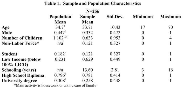
(12) We recruited adult subjects through YMCA and work recruitment centers, whose membership included many working poor. To advertise and recruit for the experiment, a brief notice was posted in low-income neighborhoods and distributed at community group meetings. (Appendix 1 contains the advertisement for participants.) A show-up fee of $12 (approximately twice the hourly minimum wage) was promised, along with on-site child care. Transportation costs were low for the participants. The experiments were conducted at four neighborhood YMCAs in Montreal, which has an extensive integrated one-price bus/subway system. We also provided a bus/subway token to those who used public transportation to return home following the experiment. Subjects volunteered for the experiment by calling ahead and agreeing to show up at a time and location identified by the experimenters. All of the experimental sessions were held in Montreal over a period of three weeks in November 2000. A total of 256 subjects participated, of which seventy-two per cent were labor market participants, either employed or unemployed.8 Sample characteristics are shown in Table 1. Average total family income for the entire sample was approximately $22,500 CAD, with 72 percent falling into the low-income category (<120% of LICO). Subjects cover a broad range of ages, from 17 to 70. The sample contains fewer men (33.2%) than women. Twelve percent are out of the labor force, and another 12 percent are full-time students. Average schooling is 13.6 years: 78 per cent held a high-school diploma, and 26 per cent reported completing a university degree. TABLE 1 ABOUT HERE. 8. Some participants who had not been targeted directly by the recruitment efforts were still able to learn about the experiment. Word of mouth about the experience and the potential for substantial sums of cash traveled fast, even in a relatively large city like Montreal. The largest group of unintended recruits was full-time students; the 31 students represent 12 per cent of the total number of subjects. Care was taken to identify this subgroup separately in the analysis.. 8.

(13) Nor were the subjects entirely without assets or access to capital markets: 26 per cent owned a car, and 54 per cent possessed a credit card. A significant fraction planned for the future: 47 per cent declared that they made regular contributions to a savings account, and 27 per cent contributed to a retirement plan. Once all participants were assembled, subjects were given their show-up fee, and the potential for additional financial compensation was explained and demonstrated.. Subjects. completed two sets of questions contained in separate booklets (with different colors): one contained 64 decision tasks, and the other contained 43 information questions. Every effort was made to make the experiment accessible and familiar to all of the subjects. Since we anticipated that this population might have little experience with research experiments or with computer interfaces, no computers were used, and transparent devices like bingo balls and dice were used to generate random draws. Special attention was paid to the visual presentation and design of the decision tasks: examples are contained in Appendix 2. To ensure comprehension, a short set of practice decision tasks was incorporated into the instruction portion of the experiment. An example of each type of decision task and the random draw process was illustrated in the sixdecision practice questionnaire. In the debriefing questionnaire, completed prior to payment, 95 per cent of the subjects indicated that they were confident they would be paid in the way that was described to them in the experiment. At the end of the experiment one of the 64 decision tasks was selected for payment using a bingo cage containing 64 balls, numbered 1 to 64. The number on the ball drawn from the cage identified the decision task for which they would be paid. If the decision involved a money prize on the same day of the experiment, the prize was given in cash, on site. Delayed payments were mailed in the form of a post-dated check for the date indicated. There were non-cash prizes such. 9.

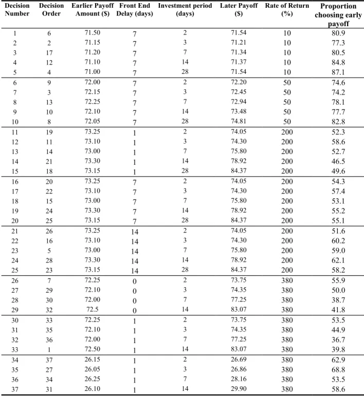
(14) as reimbursable educational expenses and guaranteed investment certificates (GICs).9 When the prize was a GIC, the experimenter signed an IOU and the prize was delivered to the subject by courier. All of the long-term GICs were purchased and distributed in early January 2001. All participants were required to sign a receipt. Each experimental session, from instruction to payoff, took about an hour and a half. For purposes of this study, we use data from three of the decision task instruments and the survey. Short time-horizon preferences are measured using a series of choices between paired amounts of money, a smaller amount sooner, v. a larger amount later, with time periods up to 28 days. Long time horizon preferences are measured in much the same way, but with larger amounts over a longer time frame, seven years. Risk preferences are measured by a series of choices between more- and less-risky gambles. Each of the instruments is described in turn. Sample decisions are contained in Appendix 2. 3.1 Short time-horizons decision tasks. Short time preferences were elicited by asking subjects whether they preferred to receive a smaller amount at an earlier date or a larger amount at a later date. Subjects were presented with the opportunity to take their payoff at some date with a specified front-end delay (FED) (e.g., two weeks from today), or to wait for a larger payoff at some later date, (e.g., two weeks and two days from today). Table 2 summarizes these 37 choices, which vary in terms of initial payoffs and alternative payoffs with respect to days lapsed and discount rates. For example, Decision 1 gave subjects the choice between $71.50 in seven days and $71.54 in nine days,. 9. A GIC is a financial instrument issued by Canadian banks. It carries a guaranteed fixed nominal rate of return, and it cannot be transferred. In addition, it cannot be redeemed before maturity except for death of the depositor. We would have like to have fixed it for more years but 7 was the longest term we could negotiate with our Canadian Bank.. 10.

(15) rewarding the subject $0.04 for waiting two additional days. This would be equivalent to a simple annual rate of return of 10 per cent. The choices in the table below involve simple annual rates of return from 10 percent to 380 percent. The investment periods are from two to 28 days, and the FED ranges from zero to 14 days. Note that decisions were not presented in the order shown here, but rather were presented one at a time in the same random order for all subjects, as revealed in the second column of the table.10 Rates of return and absolute differences were not calculated for the subjects. The last column of the table shows the proportion of subjects who chose the earlier payoff. In general we can see that subjects were more patient the larger the rate of return, and the larger the absolute return to waiting. These data are analyzed in more detail below.. TABLE 2 ABOUT HERE. 3.2 Long time-horizon time-preference choices Subjects completed a series of higher-stakes decisions, including three long-term savings decisions.11 For each of these decisions, subjects chose between a cash amount and a larger amount to be invested. For example, subjects were told, “You may choose between Option A:. 10. Coller, et al. (2003) discuss the advantages and disadvantages of scrambling the order of the questions. We now believe that scrambling is a bad idea because it results in greater inconsistency and variance of responses. In our subsequent work we have used more transparent instruments. 11 The other high stakes decisions involved choices between cash and larger amounts earmarked for own education, a family member’s education, and appliances. These decisions are discussed in our report (Eckel etal., 2002). In this paper we focus on long term saving decisions.. 11.

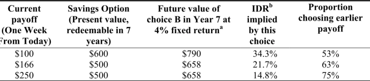
(16) $100 a week from today or Option B: $600 in your retirement plan.”12 terminology was used to emphasize the long-term nature of the investment.. The retirement In the initial. instructions, the retirement option was described as follows: “This category is money saved for your retirement. If you win this prize, you will receive a financial asset (certificate of deposit) bearing interests with a fixed maturity of 7 years.” They were not told the interest rate or the effective rate of return, but rather that the instrument was interest-bearing at market rates. This option was paid as the initial deposit to a frozen guaranteed investment certificate (GIC) redeemable in seven years, with the present value shown in column 2.. TABLE 3 ABOUT HERE. Table 3 summarizes the choices that subjects faced.13 The first two columns contain the two alternatives that the subjects actually saw: a smaller amount in cash, or a larger amount in the form of a savings certificate. The third and fourth columns indicate the future value at the prevailing interest rate of 4%, and the implied discount rate: We have calculated these values for the asset, although that information was not given to the subjects. The last column of the table shows the proportion of subjects who chose the present cash amount over the larger investment amount. Thus the choices of more than half of our subjects indicate a discount rate greater than 34.3 percent. 12. The cash alternative was offered one week from the day of the experiment to minimize the bias of mistrust. The rationale is the same for the FED employed in the short time-horizon decisions. The GIC was issued by the bank in the name of the subject after the experiment was completed. It was necessary that the subject trusted the experimenter to do this task after the completion of the experiment. If the cash alternative had been available immediately, subjects may have chosen the cash alternative rather than having to trust the experimenter. By delaying the current payoff by one week, we hold ‘trust’ constant. 13 Note that the rates of return in these questions do not match up directly with the short-term questions. That is because these questions were designed to find out how savings rates would respond to different government match rates. As mentioned previously, we are using data that were collected for a purpose other that the subject of this paper.. 12.

(17) 3.3 Risky decisions Table 4 summarizes the 14 pairs of lottery choices that were designed to elicit participants’ attitudes toward risk. The table contains the lotteries presented to the subjects, as well as properties of the lotteries. Subjects saw the decisions one at a time in the order shown. For example, the first decision (decision 38) asks subjects to choose between $60 for sure, and a 50/50 chance of $120 or $0, as shown in columns 2 and 4. Columns 3 and 5 contain the expected return and standard deviation of the gambles, which were not shown to the subjects. This series of decisions with various payoffs and levels of risk can be used to explore the risk aversion of the participants. The last column of Table 4 shows the proportion of subjects who chose the less-risky gamble (Option A). About 70 percent of subjects preferred a certain amount to a 50/50 gamble with the same expected value, regardless of the expected value. Subjects appear also to be more likely to choose the certain amount when the variance of choice B is higher. This can be seen, for example, in comparing decisions 38 and 46. In both, the option A amount is $60 for sure, and both Option B gambles have the same $60 expected payoff. The variance is higher for decision 38 and subjects are more likely to choose the safe outcome for this decision than for decision 46 (72.3% compared to 61.7%). However, even when the expected value of the gamble for Option B is higher than for option A (decisions 49-51), more than half of subjects choose the certain or lower-variance alternative. An average CRRA allowing for the main treatments and demographics is estimated in the interval censored regression summarized in Table 12 in Appendix 4.14 The CRRA values used for the regression were the values that would make the subject indifferent for each decision in Table 4. Note that for the first ten decisions this value was zero. For the interval censored 14. Much appreciation to Glenn Harrison for demonstrating the feasibility of such an approach with our limited data.. 13.

(18) regression, intervals used for analysis were (-∞, CRRA value] and [CRRA value, ∞) depending on whether the participant chose the more or less risky lottery. The predicted value of CRRA is 0.78 (standard error = 0.16) which is comparable to the results for the lab and the field. A quadrature check verifies that the model is robust.. TABLE 4 ABOUT HERE. 3.4 Information questionnaire To complete the experiment, the subjects were asked to fill out an anonymous, 43question survey. The first half of the survey contained demographic and behavioral questions (such as sex, income, education, and main activity). The second half of the survey contained attitudinal measures of subjects’ self-perceived patience, risk aversion, locus of control, and savings behavior. Several variables from this survey are used in the analysis of the decision tasks. The 43-question survey and summary statistics for the full study can be found in Appendices A and B in our working paper (Eckel, et al., 2002, available online). The questions on which variables for this study are based can be found in the appendix table of variable definitions. 4. Description of experimental measures This section describes the experimental measures used to summarize behavior in the laboratory experiment.. 14.

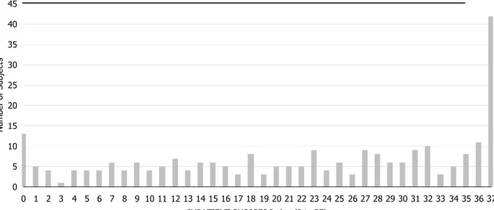
(19) To illustrate the heterogeneity of responses in the sample, we first examine a very rough measure of preferences. IMPATIENT CHOICES is the number of times each subject opted for the earliest payoff in responding to the 37 short-term time preference decisions. By choosing the sum of impatient choices, we ignore any inconsistencies in the observations, such as someone who chooses the future amount for a low rate of return and the current amount for a higher rate of return. There are many individuals that demonstrated some inconsistent decisions for this set of choices. Most occur for choices involving low returns or short time period. As mentioned earlier, the order of decisions was scrambled and there were no absolute differences or rate of return calculations made explicit to the participants. Some of the absolute differences may have appeared inconsequential to many of the participants. Many of the decisions, 17 of the 37, involved returns for waiting of less than $1 CAD. IMPATIENT CHOICES gives a general, relative time preference measure for participants. Figure 1 shows the distribution of the IMPATIENT CHOICES index. Five per cent of participants (13 subjects) exhibited the most patient behavior with IMPATIENT CHOICES = 0, while fifteen per cent of the participants (43 subjects) chose the earliest payoff regardless of payoff, discount rates, or time delays. In short, 20 per cent of the subjects were not affected by the parameters of the choices. A 380 per cent rate of return was not enough to induce 15 per cent of the sample to save, and a 10 per cent rate of return was not too low to discourage 5 per cent of the sample to save. FIGURE 1 ABOUT HERE. Because of the many inconsistent decisions, we construct a measure of time preferences for use in our analysis that uses just a few of the decisions, one for each discount rate, each with 15.

(20) the same investment period of 14 days. 14days divides subjects according to a set of discountrate intervals. We create five dummy variables, each of which corresponds to a given range of discount rates. Intervals are used rather than values because of the limited number of rates of return used in the experiment. Because this measure is constructed as a set of (0, 1) dummy variables, its use in subsequent analysis does not impose a particular functional structure on time preferences. For this measure we use only a subset of the time-preference decisions. Evidence shows that varying FED and investment period (t) can affect the elicited discount rate (see Coller and Williams, 1999). We attempt to control for this by only using 4 decisions (4, 9, 19 and 33). Decisions 4, 9 and 19 all have an investment period of 14 days and FED of 7 days. The final decision, 33, has a FED of only 1 day, but it is the longest FED we have in our decision set for a payoff of 380% and a 14-day investment period.. We use these decisions to categorize. participants into one of five groups. Twenty-four participants (9.4%) whose behavior was inconsistent (choosing not to save at high rates when choosing to save at lower rates) were dropped from the sample. 14days0-4 dummy variables were constructed in the following manner: 14days0 = 1 if subject saved in response to all four decisions, 0 otherwise (less than 10% IDR) 14days1 = 1 if subject saved in response to three decisions (9, 19, 33), 0 otherwise (IDR is at least 10% but less than 50%) 14days2 = 1 if subject saved in response to two decisions (19, 33), 0 otherwise (IDR is at least 50% but less than 200%) 14days3 = 1 if subject saved in response to one decision (33), 0 otherwise (IDR is at least 200% but less than 380%) 16.

(21) 14days4 = 1 if subject never saved, 0 otherwise (IDR at least 380%) We use these dummy variables as independent variables in our analysis of long term decisions. In addition, we construct a variable 14days to use as a dependent variable which takes on values 0, 1, 2, 3, and 4 corresponding to the categories above. To distinguish between subjects who have apparent hyperbolic preferences, we construct a variable that captures a preference for immediate payoff. PrefersToday is a (0, 1) dummy variable that takes a value of one for a participant if the participant exhibits a preference for earlier payoff more often when the early payoff is today rather than tomorrow. We use 0-day FED decisions 26-29 and 1-day FED decisions 30-33 to construct this variable. Long time-horizon IDR (LongTH) is a measure of internal discount rates implied by the subjects’ choices for long time-horizon decisions. This measure divides subjects according to a set of discount-rate intervals. We create four dummy variables, each of which corresponds to a given range of discount rates. Intervals are used rather than values because of the limited number of rates of return used in the experiment. Because this measure is constructed as a set of (0, 1) dummy variables, its use in subsequent analysis does not restrict the relative ordering of participants’ discount rates to be linear. The LongTH variable is derived from the three decisions between $X in cash and $Y “retirement investment”. Table 3 summarizes the decisions and the implied individual discount rate (IDR) for each decision. Twelve participants (4.7% of the sample) whose behavior was inconsistent (choosing not to save at high rates when choosing to save at lower rates) were dropped from the sample. LongTH variable is constructed in the following manner:. 17.

(22) LongTH= 0 if saved for all three decision tasks ($100 v. $600 GIC, $166 v. $500 GIC, $250 v. $500 GIC), the implied IDR is less than 14.8% LongTH = 1 if saved for two decision tasks ($100 v. $600 GIC and $166 v. $500 GIC), IDR is at least 14.8% but less than 21.7% LongTH = 2 if saved for one decision task ($100 v. $600GIC) (IDR is at least 21.7% but less than 34.3%) LongTH = 3 if saved for no decision task (IDR is at least 34.3%) Table 5 provides a brief summary of the proportion of participants that fall into each category of behavior for 14days, PrefersToday, and LongTH.. TABLE 5 ABOUT HERE. We now turn our attention to the determinants of the short time-horizon and relative risk attitudes measures. 5. The Determinants of Short-horizon Saving Decisions and Risky decisions 5.1 Censoring Before proceeding with our analysis, we address the issue of censoring that is presented when lab decisions may be influenced by subjects’ field opportunities. Regrettably, the field opportunities of our participants are not known. How much of a problem is this for the interpretation of the short and long-term intertemporal decisions? We argue that this lack of censoring with self-reported field opportunities may not be a substantial problem for our sample. 18.

(23) Participants will be influenced by field opportunities when they can arbitrage between the lab and the field. Preferences elicited in the lab will be influenced by participants’ field opportunities when subjects (1) are acquainted with the opportunities available in the field, (2) are able to compare lab opportunities with those in the field, and (3) are able to take advantage of the differences between field and lab rates. A recent study by Coller and Williams (1999) allows us to assess the potential importance of field censoring. Coller and Williams (1999) show that variability in the perceptions of market rates can lead to variability in the discount rates observed. Specifically, they found that when they informed participants of market rates, this reduced the residual variance of the observed discount rates. Thus informing subjects of the relevant rate appears to make them more likely to factor it into their decisions. We also know from Coller and Williams that when participants are presented with rates of return in the same terms as field opportunities, lower average discount rates are observed, which is evidence that awareness of field rates censors lab decisions. However, in our study, rate of return was not provided, nor were subjects informed about the opportunities in the field. Therefore the results from Coller and Williams should put an upper bound on the potential bias in our data. A final criterion for censoring to be a problem is that participants must be able to take advantage of the differences. It is estimated that 8-10% of Canadians with annual incomes under $25,000 do not have a bank account.15 Unfortunately, we do not know how many participants are unbanked in our sample. From the aggregate data reported in Coller and Williams, we infer that 51.7% of respondents failed to arbitrage when their self reported borrowing and lending rates indicate they had the opportunity to do so. This indicates inability or unwillingness on the part of a large fraction of the sample to engage in arbitrage between lab and field opportunities. 15. http://finservtaskforce.fin.gc.ca/research/pdf/rr12_e.pdf, see footnote 1, and see footnote 6 and 7, page 12. For US data see http://www.federalreserve.gov/dcca/newsletter/2001/spring01/unbank.htm.. 19.

(24) The lowest rate of return offered in our study was 10% for the short-horizon decisions and 14.8% in the long-horizon decisions. It is unlikely that any of our observations would be censored from below at current field rates of savings. Consider the short-horizon set of decisions (14days). In addition to the factors listed above, these decisions are less likely to be subject to arbitrage because of the relatively small monetary amounts. For 78.8 percent of the participants, their choices revealed individual discount rates of at least 50%. Given the self-reported interest rates in Coller and Williams, we can assume that none of these participants are censored by field rates for borrowing like using their credit card at 18% or even 21% interest. The other set of savings decisions, those that had the participants choose between cash one week from today and a $500 or $600 certificate of deposit, are much more likely to be subject to arbitrage opportunity because the certificate of deposit is a future payment that has collateral value. Experimental instructions stipulated that they would not have access to this money for seven years from the date the certificates would be created. Although they could use the certificates as a form of collateral, they were not informed of this fact. No participant asked if they could borrow against the anticipated certificate of deposit. 5.2 Individual Decision Data This section uses data from the short time-horizon decisions in Table 2, the risky decisions in Table 4, and survey questions to examine the determinants of the subjects’ shorthorizon saving decisions and attitude towards risk. As will be shown in Section 5 both time preference and attitude towards risk variables are related to the long time-horizon decisions of the participants. It is important, therefore, to explore the factors or contextual situations that may influence the subjects’ level of patience or tolerance of risk. We report the analysis using the two derivative measures from Section 3 above as dependent variables. In particular, we approach the 20.

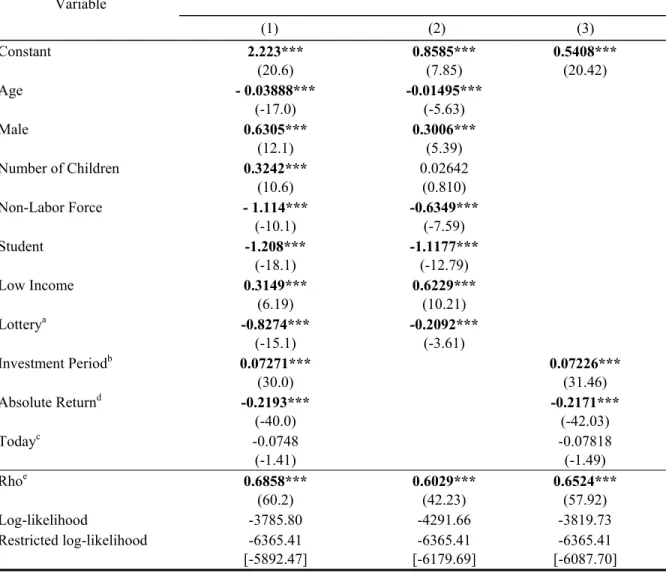
(25) question of what determines short-horizon savings decisions from several different perspectives, based on the measures described above. Table 6 reports analysis of individual decision data for all decisions. Each observation is a decision. We estimate a random-effects probit model of the individual decisions whether to choose the earlier payoff. The data set consists of 37 observations for each of 256 participants. For each observation, the dependent variable is 1 if the impatient alternative was chosen and 0 otherwise. Among the independent variables included in the regression are demographics (age, sex, and number of children), the subpopulations (Non-Labor Force participants, Student, and Low-Income), one self-reported behavioral question from the survey (Lottery), and the characteristics of the decision. We include as independent variables the information that subjects could observe when they made their decisions: Investment Period, and Absolute Return. Note we do not include rate of return as a variable for two reasons. First, subjects did not observe it, and second, it is determined by Absolute Return and Investment Period. Three specifications are presented. In column (1) all variables are included. In column (2) only individuals’ characteristics are retained. In column (3) we retained only the experiment parameters. Older subjects and women were more likely to be patient. In general, the same can be said for the Non-labor Force subgroup and the Student subgroups. Note that the Low Income subgroup was less likely to be patient and wait for a given return to savings. The absolute difference between payoffs encouraged the subjects to delay their reward. The variable Today is a dummy variable equal to 1 if the impatient payoff was the day of the experiment. It was included in this regression to test whether subjects were attracted by payoffs that were offered the day of the experiment. We find no evidence that immediate payoff was a factor in their decisions.. 21.

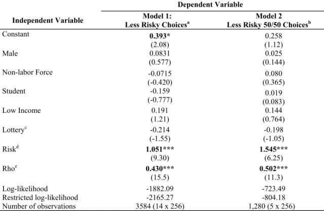
(26) An important point to note from Table 6 is the key role played by the experimental parameters in explaining the subjects’ choices of earlier payoffs (impatience). As the loglikelihood value of column (3) is closer to the one from column (1) than the specification with individuals’ characteristics only (column (2)), it is fair to recognize the greater explanatory role played by the incentives over the individuals’ characteristics in explaining the subjects’ choices of earlier payoffs.16. TABLE 6 ABOUT HERE. TABLE 7 ABOUT HERE. Table 7 reports a similar a random-effects probit model for the individual decisions whether to choose the less risky lottery. The data consist of individual decision data for each lottery choice. The dependent variable in these models is 1 if the subject chose the less-risky alternative for that decision. Model 1 includes all decisions. Model 2 includes only the decisions involving a choice between a certain outcome and a 50/50 alternative. These decisions are intuitively easier for subjects to understand, and restricting our attention to them reduces observed decision error. Independent variables Male, Non Labor Force and Student are the same as those for Table 6; age and number of children are dropped because they were consistently insignificant and their exclusion does not materially affect the remaining coefficients. The variable Risk measures the difference in the level of risk between a pair of lotteries. This. 16. Both sets of coefficients are strongly significant Test of Model 2 v.1: chi-square (3) = 1012, p<0.001. Test of model 3 v. 1: Chi-square (7) = 34, p<0.001. 22.

(27) variable is calculated as the coefficient of variation for the more risky alternative minus the coefficient of variation for the less risky alternative. (Weber, et al., 2004, show that this is the appropriate representation of how risk is perceived in decision making.) The positive and statistically significant coefficient estimate on Risk suggests that the higher the difference in the level of risk between a pair of lotteries, the greater the probability for the subject to choose the less risky lottery.. None of the coefficients for the individual. characteristics variables yielded a statistically significant estimate. For the range of risky choices we examine, incentives seem to have a significant effect on behavior, but individuals’ characteristics have weak explanatory power. 5.3 Short Horizon Savings Measures. We next turn to analysis of the data using the two alternative measures, 14days and PrefersToday (derived in section 3 above), of short-horizon saving decisions. These measures are probably cleaner measures of time preferences than the decisions to choose earlier payoffs, for reasons discussed earlier. As a reminder, participants were informed about the front end delay, the investment period, and the absolute return. However, rates of return (or discount rates) between early payoffs and alternative payoffs were not directly provided, contrary to Coller and Williams (1999) or Coller et al. (2003). Nevertheless, to compare to the existing literature, we estimate short-horizon discount rates using the same interval censored regression technique used in these studies. . The summaries of two models, with and without demographic characteristics, can be found in Appendix 4, Table 13. Average discount rates for select subgroups of the population are summarized in Table 14. Consistent with the aggregate data presented in Table 5, the estimated average short term IDR for the entire sample is 289.22% with a standard deviation of 92.8. (In interpreting these results it is important to keep in mind the large ranges of discount rates in our decision tasks.) 23.

(28) We believe that the use of the interval-censored Tobit model is less appropriate here than in the previously cited papers. The underlying response variable is latent, but we know which of the categories it belongs to. With the response variable observed only ordinally (for the 14days variable, for example, the observed responses are to choose the savings option never, once, twice and always). We use ordered probit regressions, with the dependent variable indicating the category in which the subject falls. We use ordered probit for our analysis in part because of the structure of our experiment. Table 8 reports regressions for the two types of short-horizons saving parameter ranges. The dependent variable 14days is a conversion of the dummy variable categories described above into 0, 1, 2, 3, 4 ordinal measures. The coefficients on the µ variables in this regression are the threshold parameters corresponding to the observed 14days categories. For example, the coefficient on. µ1 represents the cut-off between the categories 14days = 1 and 14days = 2.. Coefficients on the independent variables indicate that older subjects are more patient, with a discount rate more likely to fall in a lower category. Men are less patient. After controlling for low income, students are also more patient, but lower income persons are less patient. Individuals choosing the less risky lotteries are also those with higher discount rates: that is, more risk averse people are also more present-oriented. In other word risk averse individuals are also high discounters. This result contradicts van Praag and Booij (2003) who found a negative correlation between risk aversion and time preference, but is consistent with Anderhub, et al.. TABLE 8 ABOUT HERE. 24.

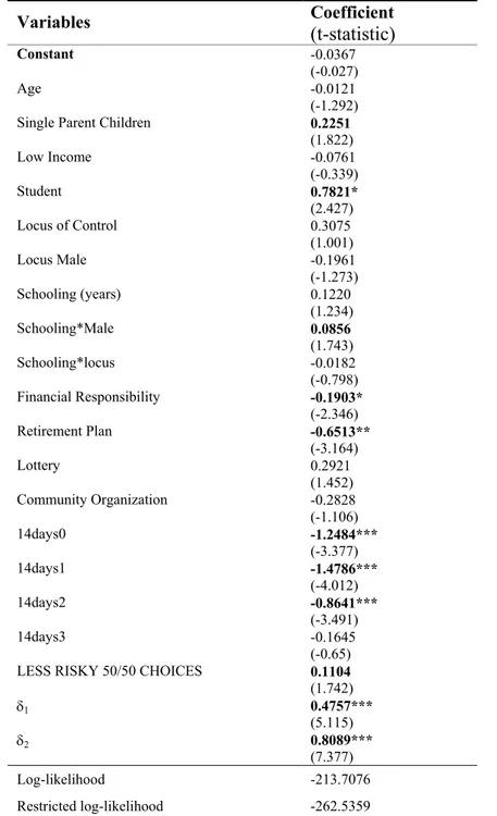
(29) Model 2 contains a similar analysis for PrefersToday, the measure extreme impatience indicating that subjects are more likely to choose the current payoff if it is today, all other things equal. This measure is only weakly related to individual characteristics, with the exception of age, where older persons are significantly less likely to exhibit this behavior. 6. Analysis of Long-horizon savings decisions Under what conditions do subjects save for the long term, for retirement or other purposes? Are short-term decisions good predictors of long-term outcomes, over and above personal characteristics?17 In the Table 9, we present the determinants of the probability that subjects will choose the cash option over the alternative of saving for retirement. We use an ordered probit model to explain the latent (unobserved) variable Ci* :. Ci* = X i β + ε i The subjects’ preferences between present and future consumption are not directly observed, but rather we only observe whether the subjects chose cash when offered over the alternative, larger amount in a “retirement savings” financial instrument.. The observed. counterpart of the latent variable Ci* is defined as follows: Ci = 0 if a participant never chose cash for any trade-off offered; Ci = 1 if $250 in cash was chosen over $500 in retirement savings (1 to 2 match rate); Ci = 2 if $166 in cash was chosen by the participant over $500 in retirement (a 1 to 3 match rate) and finally, Ci = 3 when cash were always the revealed choice of the participant for any offer of match rate in retirement savings. Note that inconsistent 17. Observed short-horizon discount rates are considerably higher than long-horizon discount rates. To estimate longhorizon discount rates we again use the interval censored regression technique described above. The summaries of two models, with and without demographic characteristics, can be found in Appendix 4, Table 15. Average discount rates for select subgroups of the population are summarized in Table 16. The estimated average long term IDR for the entire sample is 32.28%.. 25.

(30) individuals, for example, those who chose cash with a 1 to 5 match ($100 cash vs. $600 retirement savings) and not the 1 to 3 or 1 to 2 match rates were eliminated from the regressions.18 Table 9 shows results using the 14days variables as the measure of short run time preference. As the matching rate for savings increases, the choice of cash over the retirement savings instrument diminishes, as shown by the increasing coefficients on the δ1 and δ 2 , the threshold parameters for cut-offs between Ci = 1 and Ci = 2 , and between Ci = 2 and Ci = 3 , respectively. Older people, as expected, prefer long-term saving to cash. Since they are closer to retirement, saving for retirement is more salient for them. One difference between models in previous sections and this model concerns the introduction of several new variables that measure aspects of the individual’s situation that are related to their propensity to save for retirement. We substitute the variable Single Parent Children for the variables Male and Number of Children used in earlier specifications. This variable interacts Single Parent with Number of Children: It takes on a value of 0 if the person is not a single parent and the number of children if the person is a single parent. With the exception of two cases, female subjects head the single-parent households in the sample. Singleparent subjects unambiguously prefer cash to retirement savings. (When Male is added back in, it has an insignificant effect and leaves the other coefficients unchanged, leading us to believe that women who are not single parents in our sample behave much the same as men.) It is also observed that students, subjects with more schooling (in particular the men), and those that play lotteries are more likely to take the cash option. Subjects that indicate in the survey that they. 18. We use a recursive model instead of a simultaneous model of short and long-horizon saving decisions on the ground that we do not have good instruments to predict the short term variables as we saw from earlier regressions, for 14days and PrefersToday. Furthermore, these variables (14days and PrefersToday) were constructed using experimental parameters ¨Investment Period¨ and ¨Absolute return¨, for example, and therefore they can be in fact considered as already instrumented.. 26.

(31) keep track of their expenses (Expenses) are more likely to choose the retirement savings option. This last result suggests that savings seems to be facilitated when subjects operate in a structured budgeting environment. As anticipated, subjects who contribute to a retirement plan (Retirement Plan) also favour the retirement savings option. Finally, subjects reporting an association with a community group (Community Organization) have a higher probability of choosing the retirement savings option over the cash option. The coefficient estimate of LESS RISKY 50/50 CHOICES suggests that more risk-averse subjects are more likely to choose the cash option, though the effect is only statistically significant at the 10% level. Also note that subjects who purchase government-sanctioned lottery tickets are more likely to choose the cash option. To the extent that the monetary-gamble decision tasks that construct the LESS RISKY 50/50 CHOICES variable represent an adequate evaluation of the risk attitudes of the subjects, it may be that an increased level of risk aversion keeps them from investing in their retirement savings. Perhaps they view the many different situations that can arise during the seven years of fixed deposit as too risky, leading the subjects to prefer the smaller value of certain cash in the very near future to the somewhat certain benefit seven years in the future.. This pattern of behavior is also consistent with a severe cash. constraint. Subjects who appear risk averse prefer cash now to any other offered alternative. Controlling for risk attitude, the short-horizon saving decisions are significant predictors of the long-horizon saving decisions. In other words, preferences for current over future consumption that are revealed by short time-horizon decisions are strongly related to whether the subjects save for long-horizon outcomes. With ordered probit regression, the marginal effects of the regressors on the probabilities must be derived from the coefficients, whose values are difficult to interpret on their own. Table 10 summarizes the resulting probabilities of simulations run for different subgroups. The results 27.

(32) were obtained in the following manner: The probability was computed for each individual to be in each of the four categories of behaviour (Never, Once, Twice, Always Choose Cash). Then, for a specific characteristic (Single parent, Low Income, Retirement Plan), an average conditional probability with a standard deviation for each was computed. For example, the average probability for participants who have a low financial responsibility index to have a low preference for cash (never choosing cash) over retirement savings is 13.96 percent against 29.02 percent for those with a high financial responsibility index. Moving across categories of behaviour, participants with a low value of the financial responsibility index have on average a 67.61 percent probability of always taking cash at any matches but the probability drops to 48.24 percent for participants with high financial responsibility. As anticipated, subjects who do not contribute to a retirement plan (Retirement Plan) also favour the cash option. It worth noticing that subjects reporting an association with a community group (Community Organization) have a higher probability of choosing the retirement savings option over the cash option.. Perhaps being more connected with the. community provides subjects with more experience with retired persons, or perhaps community organizations explicitly encourage saving. High discounter subjects as revealed by the short-term decisions are more than twice as likely to take the cash alternative in the long-term decisions (74% vs. 30%). The coefficient estimate of LESS RISKY 50/50 CHOICES suggests that more risk-averse subjects are more likely to choose the cash option (41% vs. 62%). Finally, the results summarized in the last row of the tables, “All,” are average probabilities unconditional on specific characteristics of participants. They show the distribution of choices as a function of the estimated threshold parameters, which show the effect of the different levels of matching for saving (1 to 2, 1 to 3, or 1 to 5). 28.

(33) We have performed a similar exercise, but substituting the variable PrefersToday to represent present-biased time preferences. Results (not reported but available on request) show a quite similar pattern to the previous model in Table 9, but the PrefersToday variable has negligible statistical effect. These unreported results confirm the importance of attitude towards risk, single parenthood, years of schooling, and financial responsibility (expenses and retirement plan) in the retirement savings decision.. TABLE 9 ABOUT HERE. TABLE 10 ABOUT HERE. 29.

(34) 7. Conclusion In this paper we analyze data from an experiment that targets the working poor population in Montreal, Quebec. This population exhibits considerable heterogeneity in their preferences over a limited set of decisions designed to measure risk aversion and patience (short term and long term). We relate these measures to demographic characteristics and to each other. We find that risk-averse individuals are also more present-oriented, using both long and shortterm patience measures. While some individuals exhibit present-biased preferences in the shortrun lower-stakes measure of patience, these individuals are not present-biased in the longer-term higher-stakes decisions.. We also find that while demographic and other observable. characteristics of individuals are important correlates of discount rates, subjects are highly responsive to the parameters of the decisions. The second component of the paper focuses on an analysis whether long term savings decisions can be predicted using less-costly short-time-horizon instruments. Again we see that individual characteristics as well as responses to several survey items are significantly related to the decision to save. The correlation between long and short-term measures is significant. We tentatively conclude that relatively low-cost short-term discount rate elicitation measures can be used to predict long-term high-stakes savings behavior among the population we target, though more work is needed to establish whether this is true for other populations. An important factor in understanding the behavior of the poor may be the severe cash constraint that they face in the present. Both risk aversion and present orientation are consistent with a strong need for cash (with certainty) in the present period. Thus the elicited preferences of the poor population may be driven primarily by a need to survive in the present period. This is an issue we plan to examine further in future research. 30.

(35) Appendix 1: Advertisement for participants. We want to know what you think … and will pay big $$ for it! What is the project? We need to study how people like you make decisions. We use a simple, confidential survey to measure behaviour. In exchange for your help, you will be paid cash on site. Is it worth you trouble? We think so! You will get $12 for showing up to the survey and could make a great deal more during the survey. The survey will take at most 90 minutes to complete. Childcare is provided on site. Who can participate? We need persons whose total family income is less than $45,000 before taxes. To participate, please contact the co-ordinator as soon as possible (limited space): Jean-François Houde 985-4000 ext. XXXX. Or. Evelyne Dufort 985-4000 ext. XXXX. Who are we? CIRANO is an economic research centre based in Montreal. CIRANO is located at (address). YMCA is ….. 31.

(36) Appendix 2: instructions and sample tasks Instructions (Note instructions were available in English and French). The rules: 1. You are asked to complete two questionnaires. The first questionnaire (64 questions) is made of choice questions. The second questionnaire (43 questions) is made of information questions. All answers will be treated confidentially. 2. You win at least $12, but you can make a great deal more. 3. You must answer each question, without exception. This is the only way to win a prize. 4. If you have any questions once you have started answering the questionnaire, please raise your hand, and someone will help you. The payment procedure: Once you have answered all the questions in the survey, you will be invited to meet with me to determine the prize you win. This prize will be determined in the following manner: 1. A ball will be drawn randomly from an urn containing 64 balls, numbered from 1 to 64 representing all the choice questions of the survey. The urn does not include balls for the information questions. 2. The ball drawn identifies the question that determines your prize following your choice at that question. 3. Some monetary prizes will be given in cash; others will be mailed at a specific date. You will have to sign a receipt. In the cases of non-monetary prizes, you will receive an IOU certificate and your prize will be delivered to you by a special courier in the first weeks of January. A practice questionnaire: 1. To familiarize you with the types of choice questions of the survey, you are invited to answer 6 questions (numbered 1 to 6) of a training questionnaire. 2. Once this is done by all participants, we will draw a few balls from the urn to illustrate the payment procedure. The whole survey should take less than 90 minutes to be completed. Please note that there is no wrong or right answer, we want to know what YOU think. 32.

(37) Categories of prizes. Symbols. Cash: Money (in Canadian dollars) given to you now or at a later date. Non monetary prizes: Investment in your education and training: This category includes expenses incurred for your own education and training: admission fees at an educational institution (professional, collegial, or university), purchases of didactic material (books, software, or others). If you win this prize, we will refund your expenses made during the next year at any educational institutions. Investment in the education of a family member: This category includes expenses incurred for your children’s (or any other family member) education: admission fees at an educational institution (professional, collegial, or university), purchases of didactic material (books, software, or others). If you win this prize, your child (or any other family member) will receive a financial asset (certificate of deposit) bearing interests with a fixed maturity of 5 years. Investment in your retirement plan: This category is money saved for your retirement. If you win this prize, you will receive a financial asset (certificate of deposit) bearing interests with a fixed maturity of 7 years. Purchase or maintenance of durable goods: This category includes any expenses that you are planning to do in a near future (less than a year) and which are related to the purchase of durable goods (computer, electronic good, car, etc.) or to the maintenance of these goods (home repair, car repair, etc.). If you win this prize, you will receive a RONA gift certificate.. 33.

(38) Sample Time Preference Task:. You must choose between two payoffs A or B : Choice A: $72..50 tomorrow CHOICE B: $83.07 IN TWO WEEKS FROM TOMORROW. Remember: Today is Tuesday, November 10, 2000. Please circle your choice in the calendar. You will receive the payoff at the date of the choice you have circled. 10-nov. 11-nov $ 72.50. 12-nov. 13-nov. 14-nov. 15-nov. 16-nov. 17-nov. 18-nov. 19-nov. 20-nov. 21-nov. 22-nov. 23-nov. 24-nov. 25-nov $ 83.07. 26-nov. 27-nov. 28-nov. 29-nov. 30-nov. 1-déc. 2-déc. 3-déc. 4-déc. 5-déc. 6-déc. 7-déc. 8-déc. 9-déc. 10-déc. 11-déc. 12-déc. 13-déc. 14-déc. 15-déc. 16-déc. 17-déc. 18-déc. 19-déc. 20-déc. 21-déc. 22-déc. 23-déc. 24-déc. 25-déc. 26-déc. 27-déc. 28-déc. 34.

(39) Sample Risk Task:. You must choose A or B : If you choose A, you win $100 (100% chances); If you choose B, you will be asked to roll two ten-sided dices. If the sum of the dice indicates a number between 1 to 50 inclusively, you win $200 (50% chances). If the sum indicates a number between 51 to 100, you win nothing (50% chances). These two choices are represented by the two following graphs: $100 1. 100 $200. 1. Circle A or B according to your choice:. 0$ 50. 51. A. 100. B. 35.

(40) Sample Investment Task:. You must choose A or B : Choice A : $100 one week from today Choice B : $600 in your retirement plan These two choices are represented by the two following graphs. Please circle your choice: $ 100 one week from today. $600 in your retirement plan. Or. Choice A. Choice B. 36.

(41) Appendix 3: Variable definitions TABLE 11 ABOUT HERE. 37.

(42) Appendix 4: Tables TABLE 12 ABOUT HERE. TABLE 13 ABOUT HERE. TABLE 14 ABOUT HERE. TABLE 15 ABOUT HERE. TABLE 16 ABOUT HERE. 38.

(43) REFERENCES Anderhub, Vital, Uri Gneezy, Werner Guth and Doron Sonsino. 2001. “On the Interaction of Risk and Time Preferences: An Experimental Study.” German Economic Review 2(3), 239-252 Becker, G. M., M. DeGroot, and J. Marchak. 1964. “Measuring Utility by a Single-Response Sequential Method.” Behavioral Sciences 9: 226-232. Cameron, Lisa. 1999. “Raising the Stakes in the Ultimatum Game: Experimental Evidence from Indonesia.” Economic Inquiry 37(1): 47-59 Cameron, Trudy and Geoffrey R. Gerdes. 2003. “Eliciting Individual-Specific Discount Rates.” Department of Economics, University of Oregon, Working paper 2003-10. Coller, M., G. Harrison, and E. Rutström, 2003, "Are Discount Rates Constant? Reconciling Theory and Observation," Working Paper 3-31, Department of Economics, College of Business Administration, University of Central Florida; available at http://www.bus.ucf.edu/wp/ Coller, Maribeth and Melonie B. Williams. 1999. “Eliciting Individual Discount Rates.” Experimental Economics 2(2): 107-27 Eckel, Catherine C. and Philip J. Grossman. 2002. “Sex differences and statistical stereotyping in attitudes toward financial risk.” Evolution and Human Behavior 23(4): 281-295. Eckel Catherine C., Cathleen Johnson, and Claude Montmarquette C. 2002. “Will the Working Poor Invest in Human Capital? A Laboratory experiment.” SRDC Working Paper 0201, Ottawa. http://www.srdc.org/english/publications/workingpoor.htm Frederick, Shane, George Loewenstein, and Ted O’Donoghue. 2002. “Time Discounting and Time Preference: A Critical Review.” Journal of Economic Literature 40(2): 351-401. Harrison, Glenn W., Eric Johnson, Melayne M. McInnes, and E. Elisabet Rutström. 2003a. “Risk Aversion and Incentive Effects: Comment.” Working Paper 3-19, Department of Economics, College of Business Administration, University of Central Florida; available at http://www.bus.ucf.edu/wp/ Harrison, Glenn W., Eric Johnson, Melayne M. McInnes, and E. Elisabet Rutström. 2003b. “Individual Choice and Risk Aversion in the Laboratory: A Reconsideration.” Working Paper 318, Department of Economics, College of Business Administration, University of Central Florida; available at http://www.bus.ucf.edu/wp/ Harrison, Glenn W., Morten Igel Lau, E. Elisabet Rutström and Melonie B. Sullivan. 2004 “Eliciting Risk and Time Preferences Using Field Experiments: Some Methodological Issues.” in J. Carpenter, G.W. Harrison and J.A. List (eds.), Field Experiments in Economics (Greenwich, CT: JAI Press, Research in Experimental Economics, Volume 10); available at http://www.bus.ucf.edu/wp/. 39.

(44) Harrison, Glenn, W., Morten I. Lau, and Melonie B. Williams. 2002 “Estimating Individual Discount Rates in Denmark: A Field Experiment.” American Economic Review 92(5): 16061617 Holt, Charles and Susan K Laury. 2002, “Risk Aversion and Incentive Effects.” American Economic Review 92(5): 1644-1655. Keren, G. and P. Roelofsma, P. (1995). “Immediacy and Certainty in Intemporal Choice.” Organizational Behavior and Human Decision Processes 63: 287-297. van Praag, Bernard M.S. and A. S. Booij. (2003). “Risk Aversion and the Subjective Time Discount Rate: A Joint Approach.” CESifo Working Paper 293, University of Amsterdam. Weber, E. U., Shafir, S., & Blais, A.-R. (2004). Predicting risk-sensitivity in humans and lower animals: Risk as variance or coefficient of variation. Psychological Review 111(2): 430-445.. 40.