Directed Technical Change and International Trade

Cahier 2003-18

DUDLEY, Leonard

MOENIUS, Johannes

Département de sciences économiques

Université de Montréal

Faculté des arts et des sciences

C.P. 6128, succursale Centre-Ville

Montréal (Québec) H3C 3J7

Canada

http://www.sceco.umontreal.ca

SCECO-information@UMontreal.CA

Téléphone : (514) 343-6539

Télécopieur : (514) 343-7221

ISSN 0709-9231

DIRECTED TECHNICAL CHANGE

AND INTERNATIONAL TRADE

Leonard Dudley* Université de Montréal leonard.dudley@umontreal.ca Johannes Moenius Northwestern University j-moenius@kellogg.nwu.edu April 30, 2003 Abstract

Recent changes in comparative advantage in the largest OECD economies differ significantly from the predictions of Heckscher-Ohlin-Vanek theory. Japan's rising share of OECD machinery exports and the improvement in the comparative advantage of the USA and Germany in heavy industry were accompanied by growing scarcities of the factors used intensively in the favored sector of each country. Here we examine Acemoglu's (1998, 2002) hypothesis that technical change may be directed toward raising the marginal productivity of abundant factors. Testing this hypothesis with 1970-1992 export data from 14 OECD countries, we find evidence that international comparative advantage was reshaped by innovation biased toward the abundant factors in the largest economies.

JEL Codes: F1, O3

Keywords: international trade, comparative advantage, induced innovation, technological change, dynamic

* Leonard Dudley, Economics Department, Université de Montréal, Montréal QC Canada H3C 3J7.

Heckscher-Ohlin-Vanek (HOV) trade theory predicts that a country will tend to export the services of its most abundant factors (Vanek, 1968). Accordingly, there should be a one-to-one correspondence between changes in relative factor endowments and changes in relative factor-service exports. Yet over the last decades of the twentieth century, there were two remarkable developments in the comparative advantage of the largest trading economies that do not fit this pattern. First, between 1970 and 1992, Japan's comparative advantage in machinery relative to heavy industry rose dramatically. Its export share in this human-capital-intensive sector doubled, rising from 11 to 22 percent of the OECD total, while its share in heavy industry fell (see Table 1). However, the observed changes occurred without the expected modification in factor endowments, since the ratio of human to physical capital actually declined significantly in Japan.1 Second, the comparative advantage of both the USA and Germany rose in physical-capital-intensive heavy industry while falling in machinery. Yet in both of these countries, physical capital became scarce relative to human capital.

[Insert Table 1 about here.]

If a theory's predictions are found to be false, there are two possible reasons: either the theory is wrong or those who have tested it have omitted some vital element. The consensus view at present is that HOV theory itself is flawed. When Trefler (1993) tested this theory using an extension of Leontief's (1953) input-output methodology, he was able to reject the hypothesis of identical technology in all countries. Subsequently, in a seminal study, Trefler (1995) discovered that the productivity of a country's factors of production tended to increase with its per-capita income. Other recent studies confirm that differences in comparative advantage may be explained by something other than measured stocks of production factors. Davis, Weinstein, Bradford and Shimpo (1997) found that while the HOV model provided an excellent explanation for interregional trade in Japan, it worked poorly in explaining trade among countries. There would seem to be differences across countries that are not present when one compares regions in a single country. Thus, when Maskus (1999) applied the HOV model to the UK and the USA, he

1_{In this paper, we measure human capital in a sector by the ratio of that sector's average salary to}

obtained results compatible with inter-country differences in factor or industry productivity. Similarly, Davis and Weinstein (2001a, 2001b) demonstrated that the factor endowment differences emphasized by the H-O model explain trade well if one drops the assumption that technology is constant across countries.

Our findings are in strong contrast to this literature; they complement recent work of Harrigan (1997) and Redding (2002). Harrigan (1997) explained changes in production by sector for ten OECD countries between 1970 and 1990 by differences in factor endowments and neutral technological change. Redding (2002) analyzed changes in sectoral shares of GDP for seven OECD countries over the same period. He found that with the exception of Japan, these changes were explained by variations in factor endowments and generalized technological change. However, since neither of these studies allowed for country-specific biased technological change, they are unable to explain the empirical anomalies noted above.

Our analysis too suggests that the HOV theory is valid. However, to close the gap between the predictions of this theory and observed patterns in the trade data, we add the concept of factor-biased technical progress. In essence, we argue, the international differences in technology between countries observed in earlier studies of comparative advantage are the result of technological change that alters the marginal rate of substitution between factors. Evidence that induced innovation may be important is provided in a recent study by Popp (2002) who showed that changes in world energy prices had a significant effect on the number of patents granted for energy-efficient innovations. Since energy is traded internationally, such induced innovation should not greatly affect the comparative advantage of the industrialized countries. However, because labor, human capital and physical capital are only imperfectly mobile internationally, their relative abundance will vary across countries. Therefore, the response of entrepreneurs to conditions in local factor markets will affect comparative advantage.

In which direction will such managers search for new ideas? In the past, it was assumed that innovation would be directed toward augmenting factors whose price was high. Recently, however, Acemoglu (1998, 2001, 2002) has suggested that an additional important consideration is the size of the potential market for inventions. He argued that entrepreneurs will tend to direct

their innovative efforts toward increasing the productivity of a factor that is relatively abundant. They will tend to do so by increasing their country's effective endowment of a complementary factor. Through the Rybczynski effect, these additional effective factor endowments would tend to raise international competitiveness in those sectors intensive in the augmented factors and lower competitiveness in other sectors.

For example, a Japanese vehicle manufacturer such as Honda might seek to raise the productivity of its heavy investments in plant and equipment by developing management procedures that allow assembly-line workers to participate in product and process design and in product inspection (Sakiya, 1982). In effect, the firm would be creating effective human capital to complement abundant physical capital. To take another example, an American producer of metal products such as Nucor might take advantage of abundant university-trained workers to develop digitally-controlled production techniques that allow steel to be made efficiently from scrap metal (Barnett and Crandall, 1986). Since such mini-mills produce steel with much less equipment per ton than was previously possible, they in essence create effective physical capital.

In order to test these ideas, we introduce directed technological change into a dynamic model of comparative advantage. We do so in three steps. In Section I, we show that biased technical change offers a plausible explanation for anomalies present in the trade of the major industrialized economies. Then in Section II, we present and simulate a three-good, three-factor, two-country general-equilibrium model of world trade that provides a theoretical basis for Balassa’s (1979) empirical measure of Revealed Comparative Advantage. We show that under standard neoclassical assumptions, the model is unable to replicate the main features of world trade over the period studied. To improve the model's predictive power, we propose two changes. First, we allow previous biased technical change to raise the initial effective endowment of physical capital in one country. Second, over the simulation period, we permit directed technical change that raises the marginal productivity of each country’s abundant factor. Finally, in Section III, we use the export data of 14 OECD countries from 1970 to 1992 to test whether the main features of this simulation exercise are consistent with observed trade flows.

I. Directed Technical Change: the Evidence from Trade Flows

In this section, we examine in greater detail the puzzling evidence of important changes in comparative advantage without the changes in factor abundance required by HOV theory. We begin by presenting measures of relative abundance and comparative advantage. We then subject HOV theory to a visual test for the seven largest trading economies. Finally, drawing on recent contributions to the theory of technical change, we propose an explanation for the resulting anomalies based on the incentives of entrepreneurs to raise factor productivity selectively.

(a) Factor Abundance and RCA: the Stylized Facts

To better understand changes in trade patterns, it will be helpful to have an easy way to compare changes in relative factor abundance with changes in comparative advantage. Let us begin with a measure of relative factor abundance. Let Vi be a country's endowment of factor i

and let V be the total OECD endowment of that factor. Then the country's share of factor i is_i

i i

i V V

v / . (1.1)

The relative endowment of factor i compared with factor j, aij, in a country's endowment of the

two factors may then be expressed as the normalized difference between their shares:

. ) ( 2 j i j i ij v v v v RE (1.2)

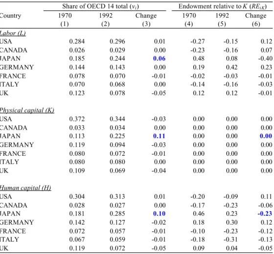
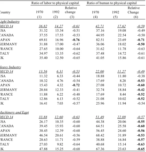
Letting H stand for human capital and K and L for physical capital and labor respectively, we may calculate REHK and RELK. Table 2 shows this measure for each of the Group of Seven

countries for 1970 and 1992. We may plot REHK against RELK for each of these countries over

the period 1970 to 1992. The resulting graphs appear on the left side of Figure 1. 2

2

The price series used by the OECD for deflating investment are in 1985 dollars. For a given country, the base-year rate is compatible with purchasing power parity. Entries for other years are calculated by means of an adjustment of the country's price series for its nominal exchange rate with the USA.

[Insert Table 2 about here.] [Insert Figure 1 about here.]

Turn now to a possible measure of comparative advantage. In a series of studies, Balassa (1965, 1979) defined the Revealed Comparative Advantage (RCA) of a country in sector i as:

E E E E x i i i / / , (1.3)

where Ei represents the country's exports of sector i, E world exports of sector i, Ei . total exports

of the country and E total world exports. If the country's share of world markets in sector i is greater than its share of total exports, then it has a comparative advantage in that sector; if the measure is less than one, the country has a comparative disadvantage in i. Note that although a country may have a comparative disadvantage in a given sector, it may still have a comparative advantage relative to another country in that sector, if the value of the first country’s RCA index is higher. Since Balassa's index of RCA has been rejected as ad hoc (Harrigan and Zakrajsek, 2000), we derive this measure directly from a theoretical model in Section II below.

Using the Balassa measure, we may define the real comparative advantage of a country in sector i relative to sector k as:

k i

ik x x

RCA

Let us then divide manufacturing industries into three groups -- machinery and equipment (X), heavy industry (Y) and light industry (Z). Table 1 shows the RCA of the Group of Seven countries in these industry groups in 1970 and 1992. The graphs on the right side of Figure 1 plot

RCAXY against RCAZY for each Group-of-Seven country relative to a larger group of 14 OECD

countries of which they are a part. Note that there were statistically significant changes in RCA, indicated by the arrows, in each of the seven countries.

The factor intensities of these three industry groups are shown in Table 3. It may be seen that heavy industry had the lowest levels of workers and human capital per million dollars of

physical capital and may therefore be considered as physical-capital-intensive. Light industry had the highest ratios of labor to physical capital and an intermediate level of human capital per physical capital and accordingly may be considered to be labor-intensive. Finally, machinery and equipment had the most human capital per million dollars of physical capital and an intermediate amount of labor. Accordingly, it may be considered to be human-capital intensive. If we can neglect the amounts of the less important factors in each sector, we see that flows of products of light industry, heavy industry and machinery provide a rough measure of exports of services of labor, physical capital and human capital respectively.

[Insert Table 3 about here]

(b) A Visual Test of HOV Theory

HOV theory predicts that the deviations from zero in the relative abundance of factors will lead to deviations in the exports of services of these factors. If the theory is correct, therefore, relative endowments shown in the left-hand graphs of Figure 1 will appear in the same

quadrant and change in the same direction as comparative advantage shown in the right-hand

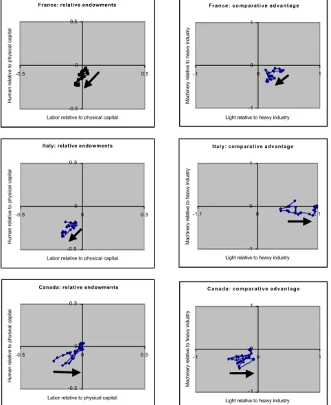
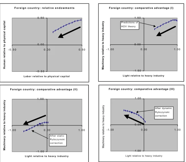
graphs. For example, to see how the graphs for Japan should appear if HOV theory is correct, consider the first two simulated graphs in the upper row of Figure 2 below. Both time series start in the upper left quadrant and descend toward the origin. Returning to the actual data in Figure 1, we see that the HOV predictions are verified for the United Kingdom, France and Canada. The clusters of points are in roughly the same position with respect to the origin in the pairs of graphs for these countries. Moreover, the arrows that indicate the directions of statistically significant changes point in the same directions.3

When one considers the largest economies, one finds important anomalies with respect to HOV theory. A first difficulty is that in the pairs of graphs of the United States, Japan and Germany, the clusters of points are in different quadrants. The discrepancy is particularly

3

In the case of Italy, the increase in physical capital relative to the other factors did not improve the comparative advantage in heavy industry. A possible explanation is that much of this investment was not in response to market forces but was rather channeled by the state into unproductive projects of publicly controlled firms such as ENI and IRI.

important for Japan. The left-hand graph shows that labor was abundant relative to physical capital. Yet Japan had a comparative advantage in heavy industry relative to light industry for most of the period studied.

A second problem concerns the direction of changes in these countries. Thanks to its very high savings rate, Japan accumulated physical capital more rapidly than any other OECD country over the period studied (see Table 2). As a result, the relative abundance of labor and human capital fell. However, as we saw at the outset of this paper, instead of becoming more specialized in heavy industry as HOV theory predicts, Japan doubled its market share in machinery and equipment.

In the United States and Germany, the movements were also in contradiction to HOV theory. With low and falling savings rates, the United States and Germany experienced a decline in the relative abundance of physical capital with respect to human capital. Yet in both countries, comparative advantage in heavy industry improved significantly relative to machinery and equipment.

Our task for the rest of the paper will be to explain these two puzzling features. The first is Japan’s initial surprising strength in heavy industry in 1970. The second is the reversal of fortunes between Japan on the one hand and the USA and Germany on the other hand in heavy industry and machinery over the period from 1970 to 1992.

(c) The Direction of Technical Change

Let us consider a possible explanation for the two anomalies discussed in the preceding section. Acemoglu (2001) distinguishes between two types of innovations. Technical change is said to augment a factor if it increases the effective amount of the factor. Let A(t) represent the technology at time t and let K and L represent capital and labor respectively. Then if the production function may be written:

], [L, A(t)K

F

Y (1.2)

Technical change is said to be biased in favor of factor L if it increases the marginal product of L relative to that of other factors.

.

0

/

/

A

K

F

L

F

Following Acemoglu (2001), let equation (1.2) take the CES form,

/ 1 ) )( 1 ( AK L Y .

Then 1/(1 )is the elasticity of substitution between L and K. The relative marginal product of L is: / 1 1 1 K L A MP MP K L

It may be seen that if the elasticity of substitution between L and K is inferior to one, an increase in A, the productivity of K, raises the marginal product of its complement, L. In this case, K-augmenting technical progress will be L-biased, since the additional effective K will raise the relative demand for L.

Might directed technical change explain the two puzzling features in recent trade patterns noted above? Consider first Japan’s initial strength in heavy industry. Acemoglu (2001) has demonstrated that in a neoclassical model that allows biased technical change, technical progress in long-run equilibrium will be labor-augmenting. However, on the transition path toward that equilibrium, capital will be relatively scarce and progress will be capital-augmenting. The explanation, offered by Kennedy (1964), is that the high rent of capital will induce capital-augmenting technical change. As shown above, if capital and labor are gross complements, capital-augmenting technical change will be labor-biased; that is, innovation will increase the

marginal product of labor. In Japan such capital-augmenting technological change in response to the relatively high price of capital during the immediate post-war decades would explain that country’s surprising success in exporting capital-intensive goods in 1970.

Might biased technical change also explain the changes in comparative advantage of Japan and the United States in the period after 1970? Assume that physical capital and human capital are complements. Acemoglu (2001) has argued that in addition to responding to relative factor prices, developers of new technologies will also be sensitive to the size of the potential market for their innovations. On the one hand, in Japan, with a high savings rate and relatively few college graduates, it would be profitable to increase the productivity of abundant physical capital through human-capital-augmenting technical change. Such technical change would be physical-capital-biased. On the other hand, in the United States, where college graduates are abundant, entrepreneurs would find it more profitable to adopt physical-capital-augmenting technologies. Accordingly, technical change there would be human-capital-biased.

In short, a model of induced innovation based on Acemoglu's theory of directed technological change offers a plausible explanation for the variation in the measured productivity of physical capital across countries in 1970. It can also explain differences in the subsequent direction of technological change between Japan and the rest of the OECD. But can such a model successfully replicate the details of observed changes in comparative advantage? We turn to this issue in the next section.

II. A 3x3x2 Model of Dynamic Comparative Advantage

In the preceding section, we developed an intuitive explanation of some anomalies in recent OECD trade data by inserting Acemoglu’s (1998, 2002, 2002) concept of directed technological change into the HOV trade theory. There is a major problem with the approach we have used this far. Our evidence on comparative advantage in Figure 1 is not from trade in factor services but rather from exports of manufactured goods. The Rybczynski theorem of course provides a link between the two types of international flows. In the case of two goods and two factors, it posits that an increase in one factor will lead to an increase in exports of the good that uses that factor intensively and a decrease in exports of the other good. However, As Deardorff (2000) has pointed out, the Rybczynski theorem is not generally valid when there are more than two factors. Moreover, the theorem holds only when the country in question is too small to affect international prices – an assumption that is surely violated for the USA and Japan.4

In this section, we extend a static 2x2x2 model proposed by Dixit and Norman (1980, 110-115) to allow for three factors and three goods. We then calibrate it to reflect the stylized facts of American and Japanese trade in 1970. Finally, we introduce factor-biased technological change into the model and examine its implications.

(a) A Static Model of Comparative Advantage

(i) The Model Structure

Assume that there are three sectors, each producing a traded good; namely, X, machinery,

Y, heavy industry and Z, light industry. There are also three factors of production, human capital, H, physical capital, K, and labor, L. Factor-price equalization is assumed to hold for effective

factors. Human capital is firm-specific; innovating entrepreneurs will therefore reap all benefits from human-capital-augmenting technological progress. Since we assume that both countries remain within the same cone of diversification, there will be no ladders of comparative

4 _{In principle, the model could also be calibrated for the 12 other countries in our sample.}

However, since the USA and Japan exhibit the most striking patterns, we limit our simulation to these two countries.

advantage such as those in Leamer (1987) and Deardorff (2001). Assume that all individuals in both countries have the following Cobb-Douglas utility function:

. 2 1 Z Y X U (2.1)

As mentioned, in the case of three factors, we cannot obtain general results analogous to those of Rybczynki (1955) unless we constrain the production technology. Is there any empirical justification for doing so? If one analyzes value added per unit of factor input in OECD countries in 1985, three features stand out. First, the coefficient of variation was highest for heavy industry (0.200), suggesting high substitutability of factors. Therefore, we chose to model this sector with Cobb-Douglas technology for our simulation exercise. This sector also had the highest ratios of physical and human capital per worker (see Table 3). Second, the lowest coefficient of variation was in light industry (0.140). Accordingly, we modeled it with a Ricardian single-factor technology. This sector also had the lowest ratios of physical and human capital per worker. Finally, the coefficient of variation was intermediate in machinery and equipment (0.188); accordingly, a Leontief technology seemed appropriate. The ratios of physical and human capital per worker were also intermediate in this sector.

On the basis of this evidence, it is not unreasonable to suggest the following set of constraints on the production functions. First, heavy industry has a Cobb-Douglas production function with substitution between human and physical capital but a fixed labor coefficient.

) , 2 min( 2 Y Y YK L H Y (2.2)

Second, light industry is Ricardian, with labor as the only input.

Z

L

Z (2.3)

Finally, machinery and equipment, has a Leontief production function with three factors but with fixed coefficients:

X X

X _{K L}

H

X min , , , (2.4)

where indicates human-capital intensity. As long as the production of X and of Y are both positive, the specifications of (2.2) and (2.4) assure that human and physical capital will be gross complements.

(ii) The integrated equilibrium

Under the assumption of competitive markets, equations (2.1) to (2.4) may be solved analytically to yield the following solution:

K KH K H K H a a KY HY 2 4 ) ( 9 ) ( 3 2 , (2.5)

where a_HY and a_KYare the inputs of human and physical capital respectively per unit of Y. Given these factor intensities we can solve for X, Y, and Z and the prices of H, K, L, Y and Z in terms of X (see the Appendix).

(iii) Equilibrium with two countries

Let the world now be divided into two countries, home (without asterisk), and foreign (with asterisk). Assume that factor-price equalization still holds. Then we may obtain the production of each good in each country. Under the Helpman and Krugman (1985) assumption of differentiated products and monopolistic competition in each sector, a given country consumes its own and the other country's production in each sector in proportion to its own share of world income. Trade flows may then be calculated from the differences between production and consumption.

(b) Revealed Comparative Advantage

Let s be the home country’s share of world income. Under the Helpman and Krugman (1985) assumption of monopolistic competition in differentiated products in each sector, the home country’s exports of product i, E , are_i

i

i sQ

E (1 ) , (2.6)

where Qi is the home country’s production of i, i = X, Y, Z. The foreign country’s exports of

product i are * * i i sQ E , (2.7)

Then from Balassa’s definition (1.3), since each country has one-half of total world exports, the Revealed Comparative Advantage of the home country in product i is

i i i i i i Q s sQ E E E x ) 1 ( 1 2 2 * * . (2.8)

In general, with three factors of production, as Deardorff (2001) observes, the Rybczynski theorem fails to hold. However, with the production structure defined here, assume that

K

H / where bars indicate world endowments; that is, industry X is human-capital-intensive and Y is physical-capital-intensive. Then, provided that both countries remain fully diversified, we have the following three propositions (see the Appendix for proofs).

Proposition 1. A country’s Revealed Comparative Advantage in the human-capital-intensive-good (X) is increasing in its stock of human capital and decreasing in its stock of physical capital.

Proposition 2. A country’s Revealed Comparative Advantage in the physical-capital- intensive good (Y) is increasing in its stock of physical capital and decreasing in its stock of human capital.

Proposition 3. A country’s Revealed Comparative Advantage in the labor-intensive good (Z) is decreasing in its stocks of human capital and physical capital.

The model was simulated with =1/2, =1, H = 0.4, K = 1, L = 1, H* = 0.38, K* = 0.44, and L* = 1. Under these assumptions, sector X (machinery) has a higher ratio of human to physical capital than Y (heavy industry). These data correspond approximately to the stylized facts of Section I. The home country represents the U.S., the foreign country Japan. Under these assumptions, the foreign country's ratio of physical capital to labor as a proportion of the world level (vK/vL), is 0.61 (= 0.113/0.185), calculated from Japan's values for 1970 in Table 2. In a

simulated replication of Japan's experience, this ratio was then raised to a final level of 0.92 (=0.225/0.244). Over the same interval, the ratio of human capital to labor in the foreign country relative to the world level was raised from 0.98 (=0.181/0.185) to 1.17 (=0.285/0.244), again replicating the Japanese data of Table 2. A comparison of the simulation in the upper-left graph of Figure 2 with the observed data for Japan in the left-hand panels of Figure 1 confirms that we have captured the main features of the historical example.

[Insert Figure 2 about here.]

Turn now to the effects of this factor accumulation on comparative advantage. The upper-right graph of Figure 2 shows the predictions of Heckscher-Ohlin theory. Although we have three factors and allow factor and product prices to vary, the directions of the change in Revealed Comparative Advantage (RCA) agree with the Rybczynski theorem. As the stock of physical capital rises relative to that of the other two factors, there is a rise in the home country's RCA in the physical-capital-intensive good and falls in its RCA in the other two goods. However, there are two serious discrepancies between these simulated results and the observed trajectories for Japan in the right-hand panel of Figure 1. A first problem is with the initial RCA levels for the

three sectors: they are far apart in the simulations but close together in the observed series. In 1970, Japan was exporting much more of the physical-capital-intensive good than Heckscher-Ohlin theory predicts. A second difficulty is with the subsequent directions of change. In the simulation, the foreign country's RCA falls in the H-intensive good relative to the K-intensive good, whereas Japan's actual RCA between these sectors moved in the opposite direction. Let us therefore investigate whether factor-biased technological change could explain these anomalies.

(c) Two Effective-Rybczynski Corrections

The static discrepancy between the simulated and actual trade patterns for Japan in 1970 may be corrected simply. Let represent the initial ratio of effective to measured physical capital in the foreign country:

* 0 * 0/ ˆ _K K (2.9)

The lower-right graph of Figure 2 shows the result. With 2, the initial values of RCA for the three sectors cluster around one in the simulations, as they do in the observed series of Figure 1. However, the subsequent trajectories for the K-intensive and H-intensive sectors still go in opposite directions to the observed series for Japan.

To correct the dynamic discrepancy, we will not attempt to model technical change explicitly. Instead, following Acemoglu (1998, 2001, 2002), we assume that the direction and rate of technical progress are determined by the initial factor endowments. As Rosenberg (2000, 10) observed, for Schumpeter (1934, 1947), the principal agency creating economic change is innovation carried out by entrepreneurs in search of greater wealth. Therefore, a straightforward way of correcting the dynamic discrepancy noted in our simulations is to allow for technological change whose direction of bias differs between the two countries. As we argued in the preceding sections, a reasonable assumption is that this bias attempted to raise the productivity of the abundant factor. The generally accepted resolution of the Leontief paradox is that during the immediate postwar decades, human capital was abundant in the USA but scarce abroad (Deardorff, 2000, 155). Then let technological change in the home country (the USA) augment

physical capital at the annual rate gK, while depleting human capital in relative terms at the rate gH. , 0 , 0 K t g t K e g K K _(2.10) . 0 , 0 H t g t H e g H H _(2.11)

Meanwhile, in the foreign country (Japan) technological change augments human capital at the annual rate g while depleting physical capital in relative terms at the rate *_H g :*_K

, 0 , * * 0 * * H t g t H e g H H _(2.12) . 0 , * * 0 * * K t g t K e g K K _(2.13)

These dynamic changes do the trick. The increase in effective human capital in the foreign country allows it to expand its production of the H-intensive good. At the same time, the augmented physical capital in the home country offsets the effect of the physical-capital deepening abroad. The lower-right graph in Figure 2 now captures the essential features of the observed Japanese trade record in Figure 1.

It now remains to be seen whether these hypotheses of static and dynamic effective-Rybczynski effects may be verified empirically.

III. Explaining Changes in Comparative Advantage

In the preceding section, we saw that two corrections were necessary to allow a neoclassical trade model to explain observed export market shares among OECD countries between 1970 and 1992. First, we introduced a static correction to augment Japan's 1970 effective capital stock; second, we made a dynamic correction to allow for country-specific endogenous technological change. We will now examine how these hypotheses might be tested, present the empirical results and discuss the relationship between these findings and previous research on technical change.

(a) Model Specification, Hypotheses and Data

Balassa (1979) proposed a two-step procedure to explain comparative advantage. Recall from equation (1.3) that xi is the Revealed Comparative Advantage (RCA) of a country in sector

i. First, for each country j, RCA by industry, xij, is regressed on industry factor intensities.

Second, the coefficients for each country from these initial regressions are regressed on the country's factor endowments. In applying this approach, Balassa used data for a single year and aggregated human and physical capital to form a single factor of production. In addition, he used factor intensities of the U.S. for all countries. Balassa (1965, 1979) and Balassa and Bauwens (1988) showed by a two-stage regression procedure that the more abundant was a country's capital stock compared to labor, the greater was its tendency to export capital-intensive goods, as predicted by the Heckscher-Ohlin theorem.5

While we retain Balassa's basic approach, we make several changes in methodology. Since very different decision processes are involved in the creation of human and physical capital, we distinguish these two forms of capital. In addition, instead of assuming a constant technology matrix for all countries, we use the observed factor intensities in each country. Finally, in order to take account of the dynamic effects of capital accumulation and technological change, we estimate a panel of 23 years rather than a cross-section of countries in a single year.

5 _{Recently, Richardson and Zhang (1999) suggested using Balassa’s measure to analyze changes}

Define the following variables:

ijt

k ratio of physical capital to labor in sector i of country j in period t divided by country j average;

ijt

h ratio of human capital to labor in sector i of country j in period t divided by country j average;

jt

K ratio of country j’s physical-capital endowment per worker to that of all countries in period t;

jt

H ratio of country j’s human-capital endowment per worker to that of all countries in period t;

J Japan dummy variable

The equation for the first step is then:

ijt ijt jt ijt jt ijt k h u x , (3.1)

where uijt is a random error.

There are two equations in the second step:

jt jt jt a b K cH * * * (3.2) jt jt jt a bK cH (3.3)

Substituting from (3.2) and (3.3) into (3.1), we obtain an initial specification of the HOV theory of comparative advantage:

x_ijt m₁k_ijt m₂K_jtk_ijt m₃H_jtk_ijt m₄h_ijt m₅K_jth_ijt m₆H_jth_ijt u_ijt, (3.4) where * 1 a m , * 2 b m , * 3 c m , m₄ a, m₅ b and m₆ c.

The first part of the Rybczynski theorem, whereby the accumulation of a factor of production leads to an increase in the production of the good intensive in that factor, is captured

by the coefficients m and₂ m . Their expected signs are both positive. The coefficients ₆ m and₃ 5

m capture the second part of the Rybczynski theorem whereby the accumulation of one factor

reduces the production of goods intensive in the other factor. Their expected signs are negative.

Consider now a variant of the preceding specification that allows for both overall physical- and human-capital-augmenting technological change and a possibly different direction of technical change in one country -- here, assumed to be Japan:

jt jt jt jt jt jt a b K c H d tK e JK f JtK * * * * * * (3.5) jt jt jt jt jt a bK cH dtH eJtH . (3.6)

Below we will allow for different directions of biased technical change in each of the sample countries. Substituting now from (3.5) and (3.6) into (3.1), we obtain a specification of the HOV theory of comparative advantage that includes directed technological change:

x_ijt m₁k_ijt m₂K_jtk_ijt m₃H_jtk_ijt m₄h_ijt m₅K_jth_ijt m₆H_jth_ijt m₇tK_jtk_ijt,

. 11

10 9

8tHjthijt m JKjtkijt m JtKjtkijt m JtHjthijt uijt

m (3.7)

From the discussion of the preceding section, the expected signs of m and ₇ m are positive and₈

negative respectively. In addition, we have added a dummy variable, J, that allows the impact of Japan's capital stock and its direction of its technological change to differ from the values for the rest of the sample. The earlier discussion leads us to expect positive signs for m9 and m11 and a

negative sign for m10.

The data come primarily from the 1994 OECD data set, International Sectoral Database. They are completed with data from the 1999 OECD source, Industrial Structure Statistics. A relatively small number of missing data points was estimated by interpolation. To measure

human capital, we used a market-based indicator. Mulligan and Sala-i-Martin (1997) suggested measuring the human capital of a skilled individual by the ratio of her wage rate to that of a worker with no schooling. Unfortunately, this measure will tend to overestimate the changes in human capital over time, since it fails to take account of the increases in physical capital available to the skilled worker that are not available to the uneducated individual. We therefore measure the average human capital per worker in a sector by the ratio of that sector's average salary to the average salary in the sector with the least-skilled workers -- textiles. By replacing the uneducated worker (for example, a street sweeper) by a textile worker in the denominator of our measure, we allow more adequately for changes in physical capital per worker over time.

The following countries were included in our sample: the United States, Canada, Japan, Germany, France, Italy, the United Kingdom, Australia, Netherlands, Belgium, Denmark, Norway, Sweden, Finland. Manufacturing was divided into the following two-digit industries: Food, Beverages and Tobacco; Textiles, Apparel and Leather; Wood Products; Paper, Paper Products and Printing; Chemical Products; Non-metallic Mineral Products; Basic Metal Industries; Metal Products; Non-Electrical Machinery; Office & Computing Machinery, Professional Goods; Electrical Machinery; Transport Equipment; and Other Manufacturing, not elsewhere specified.

(b) Results

The results of the econometric exercise can be found in Table 4. Before discussion of the results in detail, it is worthwhile to consider estimation techniques and the results as a whole. The first question to answer is of course: do the estimated coefficients have the predicted signs, and, if yes, are they statistically significant? The second, but probably even much more important question is: how robust are these results? In general, the results that are most robust to changes in specification and estimation technique are the estimates that explicitly refer to dynamic changes, namely factor-biased technical progress, and country-specific differences. The results that are less robust to changes in specification and estimation techniques are the traditional HOV variables. Although they actually always retain the correct sign, frequently they become statistically insignificant.

[Insert Table 4 about here.]

In assessing robustness, we required the data to deliver consistent results for changes in specification. The results of the standard model are presented in columns (1) and (4). Here we have controlled for country-sector specific effects in a total of 182 different categories. We then added the variables involved in our modification of the standard model in columns (2) and (5) as well as (3) and (6). We used robust standard errors for all the estimations. Because of evidence of high first-order serial correlation, we re-estimated all models using the FGLS estimator proposed by Prais and Winsten (1954). We again included country-sector dummies and used robust standard errors to evaluate the significance of the estimates.

Let us now turn to the results in detail. As stated above, the first three columns of Table 4 present the results of the estimation of equations (3.4) and (3.7) by the fixed-effects panel technique.6 Column (1) presents the simplest version with Rybczynski effects but without technological change. All coefficients have the expected signs and are statistically significant. Column (2) adds the possibility of technological change biased toward physical capital and human capital. In the OECD as a whole, technological change appears to have been biased in favor of the export of capital-intensive goods relative to human-capital intensive goods. On the average, every year, the impact of the capital stock on the propensity to export capital-intensive goods increased by 0.0045/0.115 or about four percent. At the same time there was a bias away from the export of human-capital intensive goods.

Column (3) allows for both static and dynamic country-specific Rybczynski effects. The interaction term between the Japan dummy and Kk is highly significant, indicating a higher initial productivity of physical capital in Japan than elsewhere. In addition, over the period studied, technological change seems to have been fundamentally different in Japan from the rest of the OECD. For the OECD as a whole, the positive coefficient for tKk shows that progress was

6

While a Hausmann-test suggested random-effects estimation in the case of estimation without AR(1) correction, it suggested fixed-effects estimation once we controlled for possible first-order autocorrelation. We therefore chose fixed-effects estimation to allow for better comparison

strongly physical-capital-augmenting. The negative coefficient for tHh is consistent with labor-augmenting technological change. As for Japan, the interaction coefficient of the country dummy with tKk is sharply negative. At the same time, the interaction coefficient of the country dummy and tHh is positive (though not significant). Both of these results are consistent with the hypothesis of country-specific human-capital- augmenting technological change in Japan.

In columns (4) to (6) of Table 4, the estimates are corrected for first-order autocorrelation, as described above. All signs of the coefficients of interest remain unchanged; however, the standard errors rise. Although most of the static parameters become insignificant, the Japan-specific variables and the dynamic variables introduced by our model remain significant. Note that the coefficients of the sector's human-capital intensity, h, and physical-capital intensity, k, switch signs.

Are these results robust? To answer this question, we added the terms DCTRY.Kk,

DCTRY.tKk and DCTRY.tHh where DCTRY represents a dummy variable for a country other

than Japan to the specification of column (6) in Table 4. We carried out this procedure for each of the 13 other countries. The significance levels of the initial variables did not change. However, three of the additional country coefficients were significantly different from zero at the 1 percent level. The initial capital stocks of Sweden and Finland had to be adjusted. In addition, the rate of physical-capital-augmenting technical change was different in the Netherlands from the other non-Japan countries in our sample. Nevertheless, the exercise demonstrated that the estimates of Table 4 are quite robust.

(c) Management Practices and the Direction of Technological Change

As Helpman (1999, 131-2) commented in a recent survey of empirical research on the structure of foreign trade, "any and every pattern of factor content can be explained with arbitrary differences in techniques of production." Are there any grounds for suggesting that the initial productivity level and subsequent direction of technological change might have been across estimations. The signs and degrees of significance of coefficients of the random-effects specifications of these same equations were very similar for the first three columns of table 3.

systematically different in Japan from other OECD countries in the period studied? Let us begin with the historical period and then examine more recent decades.

(i) Japanese Historical Practices

Consider first the initial 1970 discrepancy – very high exports of the physical-capital-intensive goods in Japan, a country where physical capital appeared to be scarce. Ranis (1973, 397-402), reviewing the historical evidence, showed that Japanese firms found various ways to squeeze considerably more output out of each unit of physical capital than European and American firms. One procedure was simply to have multiple shifts seven days a week with only a few hours per week for maintenance and retooling. A second procedure was to speed up the rate of production of the machines. Third, Japanese firms made more use of small-scale subcontractors who used less overhead capital per unit of output. This evidence suggests that we should correct the Hechscher-Ohlin model to allow for initial differences in the productivity of physical capital.

(ii) Recent Innovation Efforts in Japan

Turning to the question of more recent technological change, how might we explain the direction of innovative efforts in Japan in more recent decades. Aoki (1986, 1990) argued that rather than rely on the individual skills of hierarchically organized specialists, Japanese firms have developed horizontal mechanisms for sharing the knowledge of all of their work force. Ito (1992, 209-258) reviewed the differences between Japanese and American management techniques in the period we are studying. Japanese firms were more likely than their foreign counterparts to offer lifetime employment and seniority wages that increased with a worker's experience (at least up to age 55). As a result, Japanese firms were able to supplement costly formal education by the school system with low-cost learning by doing and on-site training.

Spear and Bowen (1999) noted that in the Toyota Production System, a widely applied production method in Japan, “people are the most significant corporate asset and that investments in their knowledge and skills are necessary to build competitiveness”. They also

documented in detail the learning mechanisms and the inferior role of physical capital in this production system. In the words of Ito (1992, 214), "Both blue-collar and white-collar workers in typical Japanese firms are trained more extensively than those in typical US firms, and they rotate through different jobs requiring various skills early in their careers." Although Toyota had developed these new techniques by the early 1960s, it was not until the mid-1970s that the majority of other Japanese automobile firms had followed suit (Womack et al., 1990, 68).

(ii) Recent Innovative Efforts Elsewhere in the OECD

Consider now the direction of technological change in other OECD countries. Jorgenson (2001, 3) has described in detail the remarkable declines in the relative prices of memory chips in recent decades. Between 1974 and 1996, they decreased at 41 percent per year, while other prices increased at five percent annually. These and similar capital-augmenting changes in information technology accounted for three-quarters of the increase in total factor productivity in the United States between 1973 and 1990 (Jorgenson, 2001, 25) 7.

We conclude that the hypotheses generated by the general-equilibrium simulations of Section II are supported in both the econometric tests and the historical evidence. In 1970, the productivity of physical capital in Japan appears to have been considerably higher than that in the Western economies. Moreover, subsequent to 1970, technological change in Japan would seem to have been biased in a different direction from progress in the rest of the OECD. Possibly as a result of the introduction of successive generations of information technologies based on the integrated circuit, technological change in the West was physical-capital-augmenting and, in relative terms, human-capital depleting. In Japan, from 1970 onward, technological change tended to be human-capital-augmenting and, again in relative terms, physical-capital-depleting. In both areas, the results suggest, entrepreneurial efforts led to innovations biased to increase the productivity of abundant factors.

Conclusion

Heckscher-Ohlin-Vanek (HOV) theory seems to work well in predicting trade flows at any one time between regions that share a common culture and have access to the same technology, but performs less satisfactorily when these conditions are not satisfied. In addition, the theory seems to work poorly for the world's largest economies. Two particular anomalies stand out in the trade of recent decades. First, in 1970, Japan's exports were remarkably balanced across sectors despite levels of physical capital to labor and human capital that were 40 percent lower than in other OECD countries. Second, over the following decades, Japan became increasingly specialized in machinery and equipment while the comparative advantage of the USA and Germany shifted to heavy industry relative to machinery. Yet in each case, the favored sector was intensive in the factor that became scarcer.

To explain these anomalies with respect to HOV theory, we integrated Acemoglu's (1998, 2001, 2002) theory of directed technical change into Rybczynski’s (1955) theorem of the trade impact of factor accumulation. We argued that entrepreneurs in large economies tend to bias their innovations so as to raise the productivity of the most abundant factor. In accord with the Rybczynski theorem, the resulting innovations should increase competitiveness in sectors that are intensive in the augmented factor while reducing competitiveness in sectors that are intensive in other factors.

To test this hypothesis, we extended Balassa’s (1979) methodology for explaining Revealed Comparative Advantage so as to permit three factors of production. We found evidence that Japan's 1970 effective capital stock has been underestimated. In addition, subsequent technological change in Japan tended to augment the country's endowment of human capital, whereas progress in the West augmented physical capital. In each case, the result was to raise the productivity of the most abundant factor -- physical capital in the case of Japan and human capital in the case of the USA and Germany. This evidence suggests that international comparative advantage may be shaped in part by induced innovation taken in response to the relative abundance of production factors in the largest economies.

References

Acemoglu, Daron, "Why Do New Technologies Complement Skills? Directed Technical Change and Wage Inequality," Quarterly Journal of Economics, 113 (1998), pp. 1055-1089. Acemoglu, Daron, "Labor- and Capital-Augmenting Technical Change," MIT, 2001.

Acemoglu, Daron, "Directed Technical Change," Review of Economic Studies, 69:4 (2002), pp. 781-809.

Aoki, Masahiko, "Horizontal vs. Vertical Information Structure of the Firm," American

Economic Review, 76 (1986), pp. 971-984.

Aoki, Masahiko, "Toward an Economic Model of the Japanese firm," Journal of Economic

Literature, 28 (1990), pp. 1-27.

Balassa, Bela, "Trade Liberalization and Revealed Comparative Advantage," Manchester School, 33 (1965), pp. 99-123.

Balassa, Bela, "The Changing Pattern of Comparative Advantage in Manufactured Goods,"

Review of Economics and Statistics, 61 (1979), pp. 259-266..

Balassa, Bela, and Luc Bauwens, Changing Trade Patterns in Manufactured Goods (New York: North Holland, 1988).

Barnett, Donald F., and Robert W. Crandall, Up from Ashes: The U.S. Minimill Industry (Washington D.C.: Brookings Institution, 1986).

Davis, Donald R., and David E. Weinstein, "An Account of Global Factor Trade," American

Economic Review, 91:5 (2001a), pp. 1423-1453.

Davis, Donald R., and David E. Weinstein, "Do Factor Endowments Matter for North-North Trade?," NBER Working Paper 8516, 2001b.

Davis, Donald R., David E. Weinstein, Scott C. Bradford and Kazushige Shimpo, "Using International and Japanese Regional Data to Determine When the Factor Abundance Theory of Trade Works," American Economic Review, 87:3 (1997), pp. 421-446.

Deardorff, Alan V., "Patterns of Trade and Growth across Cones," De Economist, 148:2 (2000), pp. 141-166.

Dixit, Avinash L., and Victor Norman, Theory of International Trade (Cambridge University Press: Cambridge, 1980).

Gordon Robert J., “Does the “New Economy” Measure up to the Great Inventions of the Past?”

Journal of Economic Perspectives, 4:4 (2000), pp. 49-74.

Harrigan, James, "Technology, Factor Supplies, and International Specialization: Estimating the Neoclassical Model," American Economic Review, 87:4 (1997), pp. 475-494.

Harrigan, James, and Egon Zakrajsek, "Factor Supplies and Specialization in the World Economy," Federal Reserve Bank of New York, 2000.

Helpman, Elhanan, "The Structure of Foreign Trade," Journal of Economic Perpectives, 13:2 (1999), pp. 121-144.

Helpman, Elhanan, and Paul R. Krugman, Market Structure and Foreign Trade (Cambridge, Mass.: MIT Press, 1985).

Ito, Takatoshi, The Japanese Economy (MIT Press: Cambridge, MA, 1992).

Jorgenson, Dale W., "Information Technology and the U.S. Economy," American Economic

Review, 91 (2001), pp. 1-32.

Kennedy, Charles, "Induced Bias in Innovation and the Theory of Distribution," Economic

Leamer, Edward E., "Patterns of Development in the Three-Factor, n-Good General Equilibrium Model," Journal of Political Economy, 96:5 (1987), pp. 961-999.

Leontief, W.W., "Domestic production and foreign trade: The American pattern re-examined,"

Proceedings of the American Philisophical Society, 97 (1953), pp. 332-349.

Maskus, Keith E., and Allan Webster, "Estimating the HOV Model with Technology Differences Using Disaggregated Labor Skills for the United States and the United Kingdom,”

Review of International Economics , 7:1 (1999), pp. 8-19.

Mulligan, Casey B., and Xavier Sala-i-Martin, "A Labor-Income-Based Measure of the Value of Human Capital: An Application to the States of the United States," Japan and the World

Economy, 9(2) (1997), pp. 159-91.

Popp, David, "Induced Innovation and Energy Prices," American Economic Review, 92:1 (2002), pp. 160-180.

Prais, S. and C. Winsten, “Trend Estimation and Serial Correlation.” Cowles Commission

Discussion Paper 383, Chicago, 1954.

Ranis, Gustav, "Industrial Sector Labor Absorption," Economic Development and Cultural

Change, 21 (1973), pp. 387-408.

Richardson, David J., and Chi Zhang, "Revealing Comparative Advantage: Chaotic or Coherent Patterns across Time and Sector and U.S. Trading Partner," NBER Working Paper 7212, 1999.

Redding, Stephen, “Specialization Dynamics,” Journal of International Economics, 58:2 299-334 (2002).

Rosenberg, Nathan, Schumpeter and the Endogeneity of Technology: Some American

Perspectives (London: Routledge, 2000).

Rybczynski, T. M., "Factor Endowments and Relative Commodity Prices," Economica , 22 (1955), pp. 336-341.

Sakiya, Tetsuo, Honda Motor: The Men, the Management, the Machines (Kodansha International Ltd., Tokyo, 1982).

Schumpeter, Joseph A., The Theory of Economic Development (Cambridge, MA: Harvard University Press, 1926/1934).

Schumpeter, Joseph, A., Capitalism, Socialism and Democracy, Second Edition (New York: Harper, 1942/1947).

Spear, Steven, and H. Kent Bowen, “Decoding the DNA of the Toyota Production System”,

Harvard Business Review, September-October (1999), pp. 97-106.

Trefler, Dan, "International Factor Price Differences: Leontief Was Right!," Journal of Political

Economy, 101 (1993), pp. 961-987.

Trefler, Dan, "The Case of the Missing Trade and Other Mysteries," American Economic

Review, 85:5 (1995), pp. 1029-1046.

Vanek, Jaroslav. "The Factor Proportions Theory: The n-Factor Case," Kyklos 4, (1968), pp. 749-756.

Womack, James P., Daniel T. Jones and Daniel Roos, The Machine that Changed the World (Simon & Schuster, 1990).

Table 1. Changes in export structure of Group of Seven countries, 1970 and 1992

Share of OECD 14 total Revealed Comparative Advantage

Country 1970 1992 Change 1970 1992 Change

(1)(2)(3) (4)(5)(6) Light industry USA 0.122 0.147 0.02 0.64 0.85 0.20 CANADA 0.051 0.047 0.00 0.74 1.00 0.26 JAPAN 0.101 0.030 -0.07 0.98 0.29 -0.69 GERMANY 0.112 0.156 0.04 0.63 0.81 0.18 FRANCE 0.111 0.131 0.02 1.27 1.32 0.05 ITALY 0.102 0.138 0.04 1.48 1.86 0.38 UK 0.097 0.072 -0.03 0.99 0.90 -0.09 Heavy industry USA 0.158 0.150 -0.01 0.83 0.86 0.04 CANADA 0.083 0.057 -0.03 1.21 1.22 0.02 JAPAN 0.099 0.093 -0.01 0.95 0.90 -0.05 GERMANY 0.170 0.192 0.02 0.95 1.00 0.04 FRANCE 0.089 0.111 0.02 1.01 1.12 0.11 ITALY 0.055 0.061 0.01 0.80 0.82 0.02 UK 0.089 0.090 0.00 0.91 1.12 0.21

Machinery and equipment

USA 0.240 0.195 -0.04 1.26 1.12 -0.13 CANADA 0.067 0.043 -0.02 0.97 0.92 -0.05 JAPAN 0.109 0.218 0.11 1.04 1.41 0.37 GERMANY 0.210 0.205 -0.01 1.18 1.06 -0.12 FRANCE 0.077 0.086 0.01 0.89 0.87 -0.02 ITALY 0.065 0.061 0.00 0.94 0.82 -0.12 UK 0.104 0.075 -0.03 1.06 0.94 -0.12 All sectors USA 0.191 0.173 -0.02 1.00 1.00 0.00 CANADA 0.069 0.047 -0.02 1.00 1.00 0.00 JAPAN 0.104 0.154 0.05 1.00 1.00 0.00 GERMANY 0.178 0.193 0.01 1.00 1.00 0.00 FRANCE 0.088 0.099 0.01 1.00 1.00 0.00 ITALY 0.069 0.074 0.00 1.00 1.00 0.00 UK 0.098 0.080 -0.02 1.00 1.00 0.00

Note: Small countries included in OECD14 are Australia, Netherlands, Belgium, Denmark, Norway, Sweden and Finland.

Sectors are defined from ISIC-2. Light industry: Food, Textiles, Wood and Other manufacturing;

Heavy industry: Paper, Chemicals, Non-metallic minerals, Basic metals; Machinery and equipment: Metal products, Industrial machinery, Office and computing machinery, Electrical

Table 2. Changes in factor endowments, Group of Seven countries, 1970 and 1992

Share of OECD 14 total (vi)Endowment relative to K (REiK)

Country 1970 1992 Change 1970 1992 Change

(1)(2)(3) (4)(5)(6) Labor (L) USA 0.284 0.296 0.01 -0.27 -0.15 0.12 CANADA 0.026 0.029 0.00 -0.23 -0.16 0.07 JAPAN 0.185 0.244 0.06 0.48 0.08 -0.40 GERMANY 0.144 0.143 0.00 0.19 0.42 0.23 FRANCE 0.078 0.070 -0.01 -0.02 -0.03 -0.01 ITALY 0.070 0.068 0.00 -0.14 -0.16 -0.03 UK 0.123 0.078 -0.05 0.12 0.12 -0.01 Physical capital (K) USA 0.372 0.344 -0.03 0.00 0.00 0.00 CANADA 0.033 0.034 0.00 0.00 0.00 0.00 JAPAN 0.113 0.225 0.11 0.00 0.00 0.00 GERMANY 0.119 0.094 -0.03 0.00 0.00 0.00 FRANCE 0.080 0.072 -0.01 0.00 0.00 0.00 ITALY 0.080 0.080 0.00 0.00 0.00 0.00 UK 0.109 0.069 -0.04 0.00 0.00 0.00 Human capital (H) USA 0.304 0.313 0.01 -0.20 -0.09 0.11 CANADA 0.028 0.027 0.00 -0.17 -0.23 -0.06 JAPAN 0.181 0.285 0.10 0.46 0.23 -0.23 GERMANY 0.142 0.127 -0.02 0.18 0.30 0.12 FRANCE 0.072 0.057 -0.01 -0.10 -0.23 -0.12 ITALY 0.067 0.059 -0.01 -0.18 -0.31 -0.13 UK 0.119 0.072 -0.05 0.09 0.04 -0.05

Table 3. Factor intensities by sector, Group of Seven countries, 1970 and 1992

Ratio of labor to physical capital Ratio of human to physical capital

Relative Country 1970 1992 Relative change 1970 1992 Change (1)(2)(3) (4) (5) (6) Light Industry OECD 14 36.82 14.27 -0.61 42.71 17.62 -0.59 USA 31.32 15.34 -0.51 37.16 19.08 -0.49 CANADA 37.55 17.55 -0.53 44.95 22.54 -0.50 JAPAN 69.81 16.96 -0.76 82.51 23.69 -0.71 GERMANY 31.88 17.00 -0.47 36.06 18.02 -0.50 FRANCE 27.65 10.00 -0.64 31.62 11.78 -0.63 ITALY 34.97 13.35 -0.62 37.48 14.72 -0.61 UK 35.40 12.50 -0.65 41.05 15.86 -0.61 Heavy Industry OECD 14 13.56 6.31 -0.53 22.00 11.27 -0.49 USA 11.32 6.33 -0.44 18.88 11.80 -0.38 CANADA 10.32 4.76 -0.54 17.69 8.28 -0.53 JAPAN 15.43 4.32 -0.72 27.08 10.72 -0.60 GERMANY 20.84 12.33 -0.41 32.74 18.84 -0.42 FRANCE 11.88 6.22 -0.48 17.69 8.44 -0.52 ITALY 12.86 6.13 -0.52 21.08 10.02 -0.52 UK 16.41 7.03 -0.57 25.96 11.94 -0.54

Machinery and Eqpt

OECD 14 33.88 12.60 -0.63 51.49 22.09 -0.57 USA 26.17 10.35 -0.60 44.38 20.06 -0.55 CANADA 39.45 15.93 -0.60 64.51 25.58 -0.60 JAPAN 38.45 12.39 -0.68 56.45 24.60 -0.56 GERMANY 46.54 20.61 -0.56 68.42 31.89 -0.53 FRANCE 28.63 11.71 -0.59 38.88 16.84 -0.57 ITALY 27.03 9.82 -0.64 40.68 15.14 -0.63 UK 47.88 15.25 -0.68 67.36 23.63 -0.65

Source: OECD, International Sectoral Database (1994) and Industrial Structure Statistics (1999).

Physical capital is measured in millions of 1985 $US. Human capital per worker in a given sector is defined as the average salary in that sector divided by the average salary in textiles. Total human capital in a sector is then the total number of workers in that sector multiplied by the index of human capital per worker. Sectoral averages are for the seven countries shown here along with the seven small countries mentioned in the note to Table 1.

Table 4. The determinants of Revealed Comparative Advantage, 14 OECD countries Without AR1 correction With AR1 Correction

Variable (1)(2)(3)(4)(5)(6) k 0.694** (4.78) 0.506** (3.70) 0.203 (1.21) -0.193* (-1.38) -0.225** (-1.67) -0.313** (-2.25) Kk 0.257** (2.61) 0.115 (1.21) 0.242** (2.44) 0.154 (1.26) 0.071 (0.56) 0.120 (0.92) h -0.460** (-2.25) -0.257 (-1.26) -0.059 (-0.25) 0.214 (1.10) 0.238 (1.26) 0.272* (1.40) Hh 0.726** (3.79) 0.475** (2.49) 0.414** (1.99) 0.052 (0.35) 0.058 (0.690) 0.070 (0.48) Hk -1.032** (-6.16) -0.728** (-4.78) -0.593** (-3.49) -0.160 (-1.47) -0.093 (-0.90) -0.076 (-0.77) Kh -0.155* (-1.51) -0.090 (-0.87) -0.246** (-2.30) -0.132* (-0.94) -0.130 (-0.92) -0.180 (-1.26) tKk 0.0045** (5.24) 0.0055** (5.77) 0.0052** (3.04) 0.0056** (3.22) tHh -0.0051** (-4.65) -0.0057* (-4.83) -0.0047** (-2.16) -0.0044** (-1.98) DJPN.Kk 0.713** (8.80) 0.376** (3.25) DJPN.tKk -0.018** (-5.26) -0.013** (-2.82) DJPN.tHh 0.0042 (0.98) 0.0014 (0.23) Constant 1.028** (12.79) 1.045** (13.13) 1.066** (13.74) 0.661** (5.58) 0.668** (5.74) 0.681** (5.88) 2 R 0.95 0.95 0.95 0.72 0.73 0.73 Durbin-Watson 0.23 0.23 0.23 1.75 1.75 1.75 0.88 0.88 0.88

Dependent variable: revealed comparative advantage of sector. Number of observations: 4186. Robust t-statistics in parentheses. * significant at 10% level; ** significant at 5% level; one-tailed test. Method of estimation: Columns (1)-(3) fixed effects; (4) to (6) Prais-Winsten regression with country-sector dummies.

U S A : r e l a t i v e e n d o w m e n t s

-0.5 0 0.5

-0.5 0 0.5

Labor relative to physical capital

Human relative to physical capital J a p a n : r e l a t i v e e n d o w m e n t s -0.5 0 0.5 -0.5 0 0.5

Labor relative to physical capital

Human relative to physical capital U K : r e l a t i v e e n d o w m e n t s - 0 . 5 0 0 . 5 - 0 . 5 0 0 . 5

Labor relative to physical capital

Human relative to physical capital G e r m a n y : r e l a t i v e e n d o w m e n t s - 0 . 5 0 0 . 5 - 0 . 5 0 0 . 5

Labor relative to physical capital

Human

relative

to

physical

capital

USA: comparative advantage

-1 0 1

-1 0 1

Light relative to heavy industry

Machinery relative to heavy indust r

Japan: comparative advantage

-1 0 1

-1 0 1

Light relative to heavy industry

Machinery relative to heavy industr y

UK: comparative advantage

-1 0 1

-1 0 1

Light relative to heavy industry

Machinery relative to heavy industr y G e r m a n y : c o m p a r a t i v e a d v a n t a g e - 1 0 1 - 1 0 1

Light relative to heavy industry

Machinery

relative

to

heavy