Credal Fusion of Classifications for Noisy and Uncertain Data

(1)

HAL Id: hal-01546634

https://hal.archives-ouvertes.fr/hal-01546634

Submitted on 30 Jun 2017

HAL is a multi-disciplinary open access

archive for the deposit and dissemination of

sci-entific research documents, whether they are

pub-lished or not. The documents may come from

teaching and research institutions in France or

abroad, or from public or private research centers.

L’archive ouverte pluridisciplinaire HAL, est

destinée au dépôt et à la diffusion de documents

scientifiques de niveau recherche, publiés ou non,

émanant des établissements d’enseignement et de

recherche français ou étrangers, des laboratoires

publics ou privés.

Public Domain

Credal Fusion of Classifications for Noisy and Uncertain

Data

Fatma Karem, Mounir Dhibi, Arnaud Martin, Mohamed Salim Bouhlel

To cite this version:

Fatma Karem, Mounir Dhibi, Arnaud Martin, Mohamed Salim Bouhlel. Credal Fusion of

Classifica-tions for Noisy and Uncertain Data. International Journal of Electrical and Computer Engineering

(IJECE), IAES, 2017, 7 (2), pp.1071-1087. �hal-01546634�

(2)

Credal fusion of classifications for noisy and uncertain data

Fatma KAREM

∗

, Mounir DHIBI

†

, Arnaud MARTIN

‡

, Mohamed Salim BOUHLEL

§

This paper reports on an investigation in classification technique employed to classify noised and uncertain data. However, classification is not an easy task. It is a significant challenge to discover knowledge from uncertain data. In fact, we can find many problems. More time we don’t have a good or a big learning database for supervised classification. Also, when training data contains noise or missing values, classification accuracy will be affected dramatically. So to extract groups from data is not easy to do. They are overlapped and not very separated from each other. Another problem which can be cited here is the uncertainty due to measuring devices. Consequentially classification model is not so robust and strong to classify new objects. In this work, we present a novel classification algorithm to cover these problems. We materialize our main idea by using belief function theory to do combination between classification and clustering. This theory treats very well imprecision and uncertainty linked to classification. Experimental results show that our approach has ability to significantly improve the quality of classification of generic database.

I. Introduction

There are two broads of classification technique: supervised and unsupervised one. Supervised classification is the essential tool used for extracting quantitative information based on learning database. All extracted features are assigned by labels examples. It tries to classify objects by measuring similarity between new and learning database. The second technique is based on clusters by measuring two criteria essentially compacity and separation [3,2]. It tries to form clusters which are compact and separable the possible maximum. Grouping data is not evident. Firstly clusters are overlapped most of the times. Secondly, data to classify are generally very complex. Moreover, there is not a unique quality criteria to measure the goodness of classification.

Generally, validity index is used to measure the quality of clustering. Until now, there’s no standard one which is universal. It varies from an application to another. Data to classify are not always correct especially in real applications. They can be uncertain or ambiguous. They are dependent of acquisition devices or expert opinions. Consequently, the result of classification will be uncertain. Besides, labeled examples used for training may be sometimes not available. Due to these limits and for the objective to improve classification process, we propose to combine classification and clustering. This combination also named fusion procedure aims to take account of the complementarity between both. Clustering is used to overcome problems of learning and over-fitting. Combination is made by using belief functions theory. This theory is well known in treating problems of uncertainty and imprecision.

In this paper, we report our recent research efforts toward this goal. First we present basic concepts of belief functions theory. Then we propose a novel classification mechanism based on combination. New process aims to improve classification results related to noisy environment and missing data. We conduct experiments on generic data to show the quality of data mining results. The rest of this paper is organized as follows. Related work on noise handling is discussed in Section III. In Section IV, we describe the details of proposed fusion mechanism. Experimental results and discussion are presented in Sections V. In Section VI, we conclude this paper out the future work.

II. Belief function theory

Fusion is a combination process of multiple data or information coming from different sources in order to make a decision. The final decision is better than the individual ones. The variety of information implied in the combination process makes the added value. Combination is needed in problems where ambiguity and uncertainty are big. We may be sometimes unable to make an individual decision. To raise the ambiguity, we must fuse. The applications

∗_{Research Unit SETIT , Higher Institute of Biotechnology Sfax, 3038 Tunisia, fatoumakarem@gmail.com}

†_{Assitant Professor, Research Unit PMI 09/UR/13-0, Zarroug ISSAT Gafsa 2112 Tunisia, mounir.dhibi@issatgf.rnu.tn}

‡_Professor, _University _of _Rennes _1, _UMR ₆₀₇₄ _IRISA, _Edouard _Branly _street _Bp _30219, ₂₂₃₀₂ _Lannion _Cedex

France,arnaud.martin@univ-rennes1.fr

(3)

requiring fusion are multiple. We find medicine [23] for example. Sometimes, it is difficult to do a good diagnosis disease individually. It will be better to fuse between doctors opinions. Tumor detection is the well known application. We find also image processing applications [25,21], classification [22,24], remote detection, artificial intelligence etc. The means of combination are multiple. We call it uncertain theories. We find vote theory, possibility theory, probability theory and belief function theory. The latter shows robustness in front of uncertainty and imprecision problems. The theory is invented by Dempster in 1967 and resumed by Shafer. It is also called Dempster-Shafer theory [1] [19]. Belief function theory models beliefs in an event by a function called mass function. We note by mj

the mass function of the source Sj. It is defined in the set 2Θ, their values are in [0, 1] and verify the constraint:

X

A∈2Θ

mj(A) = 1 (1)

2Θ is the set of decision or class disjunctions Ci if we talk about classification: 2Θ = {∅, {C1}, {C2}, {C1∪

C2}, . . . , Θ}. The parts A of Θ having the condition m(A) > 0 are called focal elements. The set of focal elements is

called kernel. m(A) is a measure of evidence allocated exactly to the hypothesis X ∈ A. Classes Cimust be exclusive

and not necessarily exhaustive.

Belief function theory measures imprecision and uncertainty by many functions such as credibility and plausibility. Credibility is the minimum belief. It takes account of the conflict between sources. Credibility is defined by:

Crj(X) =

X

Y ⊂X,X6=∅

m(Y ) (2)

Plausibility function measures the maximal belief in X ∈ 2Θ. We suppose that all decisions are complete so we are in a closed frame of discernment:

P lj(X) = X Y ∈2Θ_{,Y ∩X6=∅} mj(Y ) = Crj(Θ) − Crj(X c₎ = 1 − mj(∅) − Crj(Xc) (3) Xc_{is the complement of X.}

To represent a problem by the concepts of belief functions theory, we should respect three steps: modelling, combination and decision. There’s an intermediate step: discounting. It can be done before or after combination. It measures the reliability of sources. A reliability coefficient is used here noted by α. The first step is the most crucial. We must choose the suitable model to represent mass functions. It depends on the context and the application. It can be computed by many ways. We find essentially probabilistic and distance models.

For the second step: combination can be done by using different operators. The choice of the suitable operator depends on the context. Many hypotheses control the operator such as the independence and reliability of sources. We find many operators such as conjunctive, disjunctive and cautious operators or rules [14]. The first suppose that sources are independent and reliable whereas the second suppose that one of both should be reliable. The cautious rule doesn’t impose independence hypothesis for the sources. So it allows dependence and redundancy. This situation may be encountered in practice for example experts may share some information. Classifiers may be trained on the same learning sets or not separate ones.

The conjunctive combination fuse by considering the intersections between the elements of 2Θ. It reduces impre-cision of focal elements and increases belief in the elements where sources agree. If we have m mass functions to combine we have the following formula:

m(A) = (m1 m∩ 2, . . . ∩ mM)(A) = ∩ A⊂Θ(A)

= X B1∩B2,···∩BM=A M Y j=1 mj(Bj) (4)

For the cautious rule it is defined as following: m12= m1 m∧ 2= ∩ A⊂ΘA

w1(A)∧w2(A)_{= ∩}

A⊂ΘA

w12(A) ₍₅₎

(4)

m12is the information gained by the two sources S1and S2. It must be more informative than m1 and m2. If

we try to formalize this we have the following: m12 ∈ S(m1) ∩ S(m2). S(m) is the set of mass functions more

informative than m. To choose the most informative mass function we apply the least commitment principle (LCP). It is based on this principle: if several mass functions are compatible with some constraints the least informative one in S(m1) ∩ S(m2) should be selected. This element is unique it is the non dogmatic mass function (m(Ω) > 0) m12

with the following weight function:

w12(A)= w. 1(A) ∧ w2(A), ∀A ⊂ Ω (6)

w(A) is a representation of a non dogmatic mass function (simple mass function), it may be computed from m as follows:

w(A)=. Y

A⊆B

q(B)(−1)|B|−|A|+1, ∀A ⊆ Ω (7)

q is the commonality function defined as:

q(A)=. X

B⊇A

m(B), ∀A ⊆ Ω (8)

To apply this principle some informational ordering between mass functions has to be chosen. Many orderings can be used such as q-ordering and w-ordering. The first one affirms that m1is q-more committed or informative than m2

noted by

m1vqm2 (9)

if it verifies the following constraint:

q1(A) ≤ q2(A), ∀A ⊆ Θ (10)

The second one is based on the conjunctive weight function: m1is w-more committed than m2(noted by m1vw

m2) if it verifies the following constraint:

w1(A) ≤ w2(A), ∀A ⊆ Θ (11)

After calculating the mass functions and combining, we obtain the masses relative to the different elements of the frame of discernment. We must take a decision or affect a class if we have to classify at the end. It is made by using a criteria. Criterion are multiple. We mention maximum of plausibility, maximum of credibility and pignistic probability. For the first criteria, we choose the singleton or class Cigiving the maximum of plausibility. For an object

or vector x, we decide Ciif:

P lj(Ci)(x) = max

1≤k≤nP l(Ck)(x) (12)

This criteria is optimistic because the plausibility of a singleton measures the belief obtained if all disjunction masses are focused on this one. Second criteria chooses Cifor x if it gives the maximum credibility:

Crj(Ci)(x) = max

1≤k≤nCr(Ck)(x) (13)

This criteria is more selective because credibility function gives the minimum belief committed to a decision. The third criteria is between the two criterion. It moves closer credibility and plausibility. For a class Ci, the pignistic

probability is defined as:

bet(Ci) = X A∈2Θ_,C i∈A m(A) |A|(1 − m(Ci)) (14)

|A| is the cardinality of A. The maximum of pignistic probability decide Cifor an observation x if:

bet(Ci)(x) = max

1≤k≤nbet(Ck)(x) (15)

This criteria is more adapted to a probabilistic context. In the next section, we present some works related to classification combination.

(5)

III. Related works

Many researches are done about fusion in classification. Most of them is about either clustering [4,5,17,12,13] neither classification [15,19]. Some researches deploy combination to improve classification performance. Other one deploy fusion to construct a new classifier such as neural network based on belief function [7] or credal K − N N [6] or credal decision tree [8].

In [7], the study presents a solution to problems bound in bayesian model. Conditional densities and a priori probabilities of classes are unknown. They can be estimated from learning samples. The estimation is not reliable especially if the set of learning database is small. Moreover, it can not represent very well uncertainty connected to class membership of new objects. If we dispose of few labeled examples and we have to classify new object which is very dissimilar of other ones uncertainty will be big. This state of ignorance is not reflected by the outputs of statistical classifier. This situation is met in many real applications like medicine: diagnosis disease. So it tries to measure uncertainty bound to the class of the new object considering the information given by the learning data. Suppose that we have a new object to classify, we focus on his neighbors. They are considered as evidence elements or hypotheses about class membership of the new one. Masses are assigned to each class and for each neighbor of the new object to classify. The beliefs are represented by basic belief assignment and combined by Dempster-Shafer theory to decide to which class it belongs to. The study doesn’t depend strongly of the number of neighbors.

In [8], decision tree (classifying two classes) are combined to solve multi-class problem using belief function theory. Classic decision trees bases on probabilities. They are not always suitable to some problems like uncertainty. Uncertainty of inputs and outputs can not be modelled very well by probability. Moreover, a good learning database is not always available. The research proposes an extension to a previous study dealing with decision tree solving two class problem. It is based on belief function. The new study aims to treat multi-class problem by combining decision trees (two class problem) using evidence theory.

In [11], two supervised classifier are combined which are Support Vector Machines and K-Nearset neighbors. Combination aims to improve classification performance. Each of them has disadvantages. SV M for example de-pends strongly on learning samples. It is sensitive to the noise and the intruder. K − N N is a statistical classifier. It is also sensitive to noise. A new hybrid algorithm is proposed to overcome the limits of both classifiers. Concerning the combination of clustering, many researches are done. In [4], a novel classifier is proposed based on a collaboration between many clustering techniques. The process of collaboration takes place in three stages: parallel and independent clusterings, refinement and evaluation of the results and unification. The second stage is the most difficult. Correspon-dence between the different clusters obtained by the classifiers is looked. Conflict between results may be found. An iterative resolution of conflict is done in order to obtain a similar number of clusters. The possible actions to solve conflicts are fusion, deletion and split of clusters. After that, results are unified thanks to vote technique. Combination was used to analyze multi-sources images. Fusion was needed because sources are heterogeneous.

In [18], many techniques of clustering collaboration are presented. It differs by the type of result. Result can be a unique partition of data or an ensemble of clustering results. For the first type of result, fusion techniques of clas-sification are used. For the second, multi-objective clustering methods are used. They try to optimize simultaneously many criteria. At the end of process, the set of results is obtained. It is the best result that compromises between the criteria to be optimized. Concerning fusion between clustering and classification many researches deploy clustering in the learning phase of supervised classification [10,16,20].

IV. Fusion mechanism

This work is an improvement of a previous one. The former [9] was established to combine clustering and clas-sification in order to improve their performance. Both has difficulties. For clustering, we have essentially problems of complex data and index validity. For classification, we have problem of lack of learning database. We used belief function theory to fuse. We respect the three steps of combination process: modelling, combination and decision. Our frame of discernment is: 2Θ, Θ = {q. j; j

.

= 1, . . . , n} where n number of classes qj found by the supervised

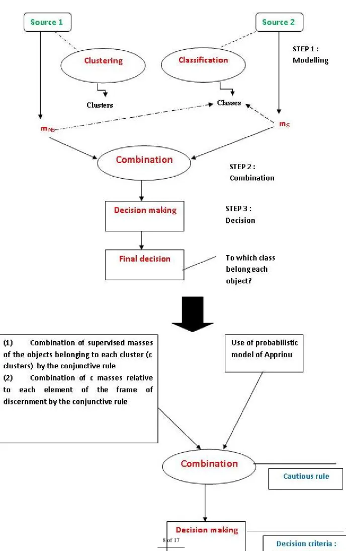
classifier. For modelling step, both sources must give their beliefs in the classes. Unsupervised source gives as outputs clusters. The classes are unknown for it. How can the clustering source give their beliefs for it? To do that, we look for the similarity between classes and clusters. More the similarity is big more the two classifications agree with each other. Generally to measure similarity we use distance. If we try to measure distance between a cluster and a class, we will confront a big problem which is the choice of the best distance. We chose to look for the recovery between clusters and classes. More they have objects in common more they are similar. Concerning supervised source, we used probabilistic model of Appriou. Only singletons interested us. In the combination phase, we adopted the conjunctive rule. It works in the intersections of the elements of the frame of discernment. At the end, we must decide to which class belong each object. The decision is made by using a criteria. We decide following the pignistic criteria. It

(6)

compromises between credibility and plausibility. To summarize the process, we have the followings: Step 1: Modelling

Masses are computed for both sources supervised and unsupervised: • Clustering (unsupervised source):

We look for the proportions of found classes q1, . . . , qnby the supervised classifier in each cluster [5,4]. ∀x ∈

Ciwith c the number of clusters found. The mass function for an object x to be in the class qjis as follows:

mns(qj) =

|Ci∩ qj|

|Ci|

(16)

where |Ci| the number of elements in the cluster Ciand |Ci∩ qj|, the number of elements in the intersection

between Ciand qj. Then we discount the mass functions as follows, ∀A ∈ 2Θby:

mnsαi(A) = αimns(A) (17)

mαi

ns(Θ) = 1 − αi(1 − mns(Θ)) (18)

The discounting coefficient αi depends on objects. We can not discount in the same way all the objects. An

object situated in the center of a cluster is considered more representative of the cluster than another one situated in the border for example. The coefficient αiis defined as (viis the center of cluster Ci):

αi= e−kx−vik

2

(19) • Classification (supervised source):

We used the probabilistic model of Appriou:

mj_s(qj)(xk) = αijRsp(qi|qj) 1 + Rsp(qi|qj) (20) mjs(qjc)(xk) = αij 1 + Rsp(qi|qj) (21) mj_s(Θ)(xk) = 1 − αij (22)

qi the real class, αij reliability coefficient of the supervised classification concerning class qj. Conditional

probabilities are computed from confusion matrices on the learning database:

αij= max p(qi|qj)(i ∈ 1, ..., n) (23)

Rs= max ql

(p(qi|ql))−1(i, l ∈ 1, ..., n) (24)

Step 2: combination

Use of conjunctive rule equation4

Step 3: decision

Use of pignistic criteria equation15

Three improvements are aiming in the present paper: noise, missing data (uncertain data) and lack of learning database. In the previous work we have supposed that data are correct. To do so, we introduce certain modifications to the previous mechanism. To compute masses for the supervised source we keep Appriou’s model20,21,22. For the unsupervised source, we follow the next steps:

(7)

∀xk ∈ Ci, A ∈ 2Θ, mi(A)

. = \

xk∈Ci

mAs(A)(xk) (25)

Thanks to that, we have an idea of the proportion of labels present in a cluster. What’s the majority class and minority ones.

Step 2: We obtain c masses for each element A ∈ 2Θ_{with c number of clusters obtained. We combine them by}

the conjunctive rule. We can view how the two classifications agree with each other. More the masses tend to 1 more they are not in conflict. Before combining, we discount masses using a reliability coefficient noted by degnetik.

∀xk∈ Ci, A ∈ 2Θ, mkns(A) . = \ s=1,...,c mdegnetik s (A)(xk) (26)

We obtain the faith in the elements of the frame of discernment.

degnetikis a measure of neatness of object xk relatively to cluster Ci. Object xkmay be clear or ambiguous for

a given cluster. If it is in the center of a cluster or near to, it is considered a very good one. It represents very well the cluster. We can affirm that it belongs to only one cluster. If it is situated in the border(s) between two or many clusters it may not be considered as clear object for only one cluster. It is ambiguous. It may belong to more than only one group. The computation of degnetiktakes account of two factors: degree of membership to cluster Ciand

the maximal degree of overlapping in the present partition noted by Smax. It is the maximal similarity in the partition

(found by the clustering).

degnetik= 1 − degoverli (27)

degoverliis the overlapping degree to cluster Ci. It is computed as follows:

degoverli= (1 − µik) × Smax (28)

Degree of neatness is the complement to 1 of the degree of overlapping. It is composed of two terms: first one (1−µik) measures the degree of not membership of a point xkto a cluster Ci. Second one takes account of overlapping

aspect. Smaxmeasures the maximal overlapping in the partition. It is computed as follows:

Smax

.

= max(S(Ci, Cj)) (29)

The clusters Ciand Cjare considered as fuzzy not hard sets.

S(Ci, Cj) = max xk∈X

(min(µCi(xk), µCj(xk)) (30)

Similarity measure is not based on distance measure due to its limits. In fact, we can find two clusters having the same distance separating them but are not separable in the same way. It is based on membership degree. We look for the degree of co-relation between two groups. What’s the minimum level of co-relation guaranteed. The new measure satisfies the following properties:

Property 1 1: S(Ci, Cj) is the maximum degree between two clusters.

Property 2: The similarity degree is limited, 0 ≤ S(Ci, Cj) ≤ 1

Property 3: If Ci . = Cjthen S(Ci, Cj) . = 1 and if (Ci∩ Cj . = ∅) then S(Ci, Cj) . = 0. Property 4: The measure is commutative, S(Ci, Cj)

.

= S(Cj, Ci)

For example, if S(Ci, Cj)

.

= 0.4 so the two clusters are similar or in relation with minimum degree of 0.4. They are not connected with a degree of 0.6.

Smax= max( max. xk∈X

(min(µCi(xk), µCj(xk)))) (31)

degnetik

.

= 1 − (1 − µik) × Smax (32)

The degree of membership of an object xkto a cluster Ciis calculated as follows:

µik . = c X l=1 ((kxk− vik) (2/(m−1)) (kxk− vlk)(2/(m−1)) )−1 i= 1, . . . , c; k. = 1, . . . , n. 1 (33) 6 of 17

(8)

where vithe center of cluster Ci, n1 number of objects. For the combination phase, we use the cautious rule5.

Sources are not totally independent because computation of masses for the unsupervised source is based on classes given by supervised sources. So, we can not say that they are independent. At the end, we decide using the pignistic probability. We are interested only in singletons: labels given by the classification. To summarize the process of fusion we illustrate that by the following figure:

V. Experimental study

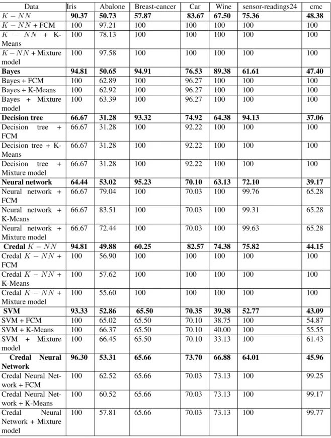
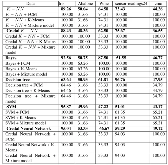
In this section, we present the obtained results for our fusion approach between supervised classification and unsupervised classification. We conduct our experimental study on different databases coming from generic databases obtained from the U.C.I repository of Machine Learning databases. We did experiments on data. We make data missing. Also, we inject noise with different rates and we take a little sampling database (10%). The aim is to demonstrate the performance of the proposed method and the influence of the fusion on the classification results in a noisy environment and with missing data. The experience is based on three unsupervised methods such as the Fuzzy C-Means (FCM), the K-Means and the Mixture Model. For the supervised methods, we use the K-Nearest Neighbors, credal K-Nearest Neighbors, Bayes, decision tree, neural network, SVM and credal neural network. We show in the Table2the obtained classification rates before and after fusion for the new mechanism. The data shown are: Iris, Abalone, Breast-cancer, car, wine, sensor-readings24 and cmc. The first ones (before fusion) are those obtained with only supervised methods (K-Nearest Neighbors, credal K-Nearest Neighbors, Bayes, decision tree, neural network, SVM and credal neural network). The learning rate is equal to 10%. We show in the Table3the obtained classification rates before and after fusion for the new mechanism for missing data. The data shown are: Iris, Abalone, wine, sensor-readings24 and cmc. The first ones (before fusion) are those obtained with only supervised methods (K-Nearest Neighbors, credal K-Nearest Neighbors, Bayes, decision tree, SVM and credal neural network). The learning rate is equal to 10%. We show in the Tables4,5,6,7,8and9the obtained classification rates before and after fusion for the new mechanism in a very noisy environment. We vary the noise levels. We show results obtained with the following levels: 55%, 65% and 70% respectively for: IRIS, Abalone, Yeast, wine, sensor-readings4 and sensor-readings2. A. Experimentation

The number of clusters may be equal to the number given by the supervised classification or fixed by the user. The tests conducted are independent for the three levels of noise. It means that they were not made in the same iteration of the program. In the following, we present the data (table1) and the results obtained (tables2,3,4,5,6,7,8and9).

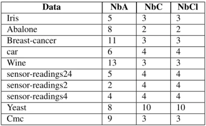
Table 1. Data characteristic NbA: Number of attributes, NbC: number of classes, NbCl: number of clusters tested

Data NbA NbC NbCl Iris 5 3 3 Abalone 8 2 2 Breast-cancer 11 3 3 car 6 4 4 Wine 13 3 3 sensor-readings24 5 4 4 sensor-readings2 2 4 4 sensor-readings4 4 4 4 Yeast 8 10 10 Cmc 9 3 3 B. Discussion

If we look to the results shown in table2. We remark the following results for each data: 1. Iris

The performance obtained after fusion are equal to 100% exception are for decision tree and neural network no improvement. The classification rate is approximately 66%.

(9)

Figure 1. fusion mechanism 8 of 17

(10)

2. Abalone

The performance obtained after fusion are better than that obtained before fusion exception is for decision tree no improvement. The classification rate is 31.28%. The best result obtained is for KNN with mixture model 97.58%.

3. Breast-cancer

The performance obtained after fusion are equal to 100% (KNN, Bayes, decision tree, neural network, credal KNN) exception are for SVM and credal neural network. The classification rate is approximately 65%. 4. car

The classification rate after fusion is better for most cases equal to 100% (KNN and credal KNN), 96% (Bayes), 92% (Decision tree). For SVM, neural network and credal neural network the performance is less than that before fusion equal to 70%.

5. wine

The classification rates obtained after fusion are equal to 100% (KNN, Bayes, decision tree, neural network, credal KNN), 73% for credal neural network, approximately 40% for SVM.

6. sensor-readings24

The classification rates obtained after fusion are equal to 100% (KNN, Bayes, decision tree, credal KNN, SVM) and to 99% for neural network.

7. cmc

We obtain 100% in most cases (KNN, Bayes, decision tree, credal KNN), 99% for credal neural network, 65% for neural network, 55% and 61% for SVM.

For the results obtained with missing data, we remark the following in table3: 1. Iris

Classification rates after fusion are excellent equal to 100% (KNN, Bayes, neural network, SVM, credal KNN, credal neural network) and to 64% for decision tree.

2. Abalone

The performance obtained after fusion is equal to 100% (credal KNN), 63% (Bayes) better than that before fusion. No improvement for KNN, decision tree, SVM, credal neural network 31%.

3. wine

The best classification rate was obtained for Bayes (100%). For credal KNN, decision tree, credal neural network no improvement was remarked.

4. sensor-readings24

The classification rates obtained after fusion are equal to 100% (KNN, Bayes, decision tree, credal KNN), to 61% (SVM) and to 94% for credal neural network.

5. cmc

We obtain 100% in most cases (KNN, credal KNN, Bayes, credal neural network), 65% for SVM. For decision tree, the rate is 34% worse than before fusion.

In a noisy environment (tables4,5,6,7,8and9), we remark the following results: 1. Iris

• Noise level equal to 55%: we remark a little improvement for KNN (33%), credal neural network (66%). For credal KNN, the performance is worse.

• Noise level equal to 65%: Classification rates after fusion are better than that before fusion (66%, 33%). • Noise level equal to 70%: No improvement for the three classifiers (33%).

2. Abalone

• Noise level equal to 55%: the best classification rate was obtained with KNN (100%). For the others, we obtain 68% (credal KNN) and 63% (credal Neural Network).

(11)

• Noise level equal to 65%: We have 63% for KNN and credal KNN, 100% (credal Neural Network). • Noise level equal to 70%: A little improvement was remarked for KNN and credal KNN 36% and 31%

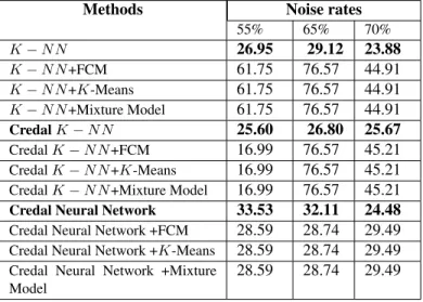
for credal Neural Network. 3. Yeast

• Noise level equal to 55%: Only the combinations of KNN has improved the performance of classification 61% while it was of 26% before fusion.

• Noise level equal to 65%: No improvement was remarked for the combination of credal neural network while it is for KNN and credal KNN. A good result equal to 76%.

• Noise level equal to 70%: All combinations have improved performance. The three tests are independent. 4. Wine

• Noise level equal to 55%: Combinations of KNN has improved perfectly the performance. We reach 100% (KNN), 73% (credal KNN). No improvement was remarked for credal neural network.

• Noise level equal to 65%: All combinations have improved performance: 100% (credal KNN), 73% (credal Neural Network) and 39% (KNN).

• Noise level equal to 70%: Improvements are shown only for credal KNN (100%), credal Neural Network (73%).

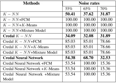
5. sensor-readings4

• Noise level equal to 55%: Only combinations of KNN and credal KNN has improved performance (100% and 85%).

• Noise level equal to 65%: We reach a performance rate of 100% for KNN and credal Neural Network and of 85% for credal KNN.

• Noise level equal to 70%: KNN has perfectly improved performance. We have 100%. Credal KNN has 78%. No improvement was remarked for credal neural network.

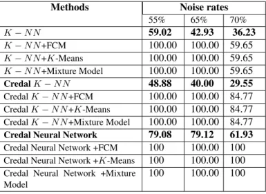
6. sensor-readings2

• Noise level equal to 55%: We have a perfect performance 100% for all combinations. • Noise level equal to 65%: same remark as before (100% for all combinations). • Noise level equal to 70%: All combinations have improved performance.

VI. Conclusion

This paper proposes a new approach which improves a previous work [9]. The goal is to construct a fusion mechanism robust to noise,lack of sampling data and missing data. The former fused both types of classification in order to overcome limits and problems linked to. It improved the performance of classification. It was based on belief function theory. The new one is based also on the same theory. Modifications were made in the phase of modelling and combination. We changed the way of calculus of masses for the unsupervised source. We modified the conjunctive rule by the cautious rule. In fact both sources are not independent. Computation of masses for the clustering is based on classes carried out by the supervised classifier. We made our experimentation in three steps. The first step, experiments are done without noise. The second one was conducted with missing data. The last one was made with different levels of noise. We showed in this paper big levels: 55%, 65% and 70%. The sampling rate is little 10%. The three tests are independent. The results obtained are good. In most cases, combinations are the best. This work can be spread by studying dependence issue deeply.

References

[1] A. Appriou, Décision et Reconnaissance des formes en signal, Chapter ”Discrimination multisignal par la théorie de l’évidence”,Hermes Science Publication, 2002.

[2] C. Blake and C. Merz Repository of Machine Learning Databases UCI, 1998. [3] M. Campedel, Classification supervis´ee, Telecom Paris 2005.

(12)

[4] G. Forestier, C. Wemmert and P. Ganc¸arski, Multisource Images Analysis Using Collaborative Clustering, EURASIP Journal on Advances in Signal Processing, vol. 11, pp. 374-384, 2008.

[5] P. Ganc¸arski and C. Wemmert, Collaborative multi-strategy classification: application to per-pixel analysis of images, In Proceedings of the 6th international workshop on Multimedia data mining: mining integrated media and complex data, Vol. 6, pp. 595-608, 2005.

[6] T. Denoeux, A k-nearest neighbor classification rule based on Dempster-Shafer Theory, IEEE Transactions on Systems, Man and Cybernetics, Vol.25, N. 5, pp. 904-913, 1995.

[7] T. Denoeux, A Neural Network Classifier Based on Dempster-Shafer Theory, IEEE Transactions on Systems, Man and Cyber-netics, Vol.30, N. 2, pp. 130-150, 2000.

[8] N. Sutton-Charani, S.Destercke and T. Denoeux, Classification Trees Based on Belief Functions, In Proceedings of the 2nd international Conference on the Belief Functions theory and Applications , Vol.164, pp. 77-84, 2012.

[9] F.Karem, M.Dhibi and A.Martin, Combination of Supervised and Unsupervised Classification Using the Theory of Belief Functions, In Proceedings of the 2nd international Conference on the Belief Functions theory and Applications , Vol.164, pp. 85-92, 2012.

[10] M. Guijarro and G. Pajares, On combining classifiers through a fuzzy multi-criteria decision making approach: Applied to natural textured images,Expert Systems with Applications, Vol. 39, pp. 7262-7269, 2009.

[11] W.Li ,D. Miao and W. Wang Two-level hierarchical combination method for text classification, Expert Systems with Applica-tions, Vol. 38, pp. 2030-2039, 2011.

[12] M. Masson and T. Denoeux, Clustering interval-valued proximity data using belief functions, Pattern Recognition, Vol. 25, pp. 163-171, 2004.

[13] M. Masson and T. Denoeux, Ensemble clustering in the belief functions framework, International Journal of Approximate Reasoning , vol. 52, num. 1, pp. 92-109, 2011.

[14] B. Quost, M. Masson and T. Denoeux, Classifier fusion in the Dempster-Shafer framework using optimized t-norm based combination rules, International Journal of Approximate Reasoning , vol. 52, num. 3, pp. 353-374, 2011.

[15] L. Xu, A. Krzyzak, and C.Y. Suen, Methods of combining multiple classifiers and their applications to handwriting recogni-tion,IEEE Transactions on Systems, Man, and Cybernetics, Vol. 22, N. 3, pp. 418-435, 1992.

[16] M. K. Urszula and T. Switek, Combined Unsupervised-Supervised Classification Method, In Proceedings of the 13th Inter-national Conference on Knowledge Based and Intelligent Information and Engineering Systems: Part II, Vol. 13, pp. 861-868, 2009.

[17] C. Wemmert and P. Ganc¸arski, A Multi-View Voting Method to Combine Unsupervised Classifications, In Proceedings of the 2nd IASTED International Conference on Artificial Intelligence and Applications, Vol. 2, pp. 447-453, 2002.

[18] C. Wemmert, Clustering collaboratif et connaissances expertes - Application `a l’analyse d’images, HDR, Strasbourg Univer-sity, 4 july 2012.

[19] A. Martin, Comparative study of information fusion methods for sonar images classification, In Proceeding of the 8th Inter-national Conference on Information Fusion, Vol. 2, pp. 657-666, 2005.

[20] Y. Prudent and A.Ennaji, Clustering incrémental pour un apprentissage distribué : vers un système volutif et robuste, In Conférence CAP, 2004.

[21] B. Belkhaoui, A. Toumi, A. Khenchaf, A. Khalfallah and M. S. Bouhlel, Segmentation of radar images using a combined watershed and Fisher technique,In Proceedings of the 6th International Conference on Sciences of Electronics, Technologies of Information and Telecommunications (SETIT), pp. 400-403, 2012.

[22] H. Dawood, H. Dawood and P. Guo, Combining the contrast information with LPQ for texture classification, In Proceedings of the 6th International Conference on Sciences of Electronics, Technologies of Information and Telecommunications (SETIT), pp. 380-385, 2012.

[23] W. Aribi, A. Khalfallah, M. S. Bouhlel and N. Elkadri, Evaluation of image fusion techniques in nuclear medicine, In Pro-ceedings of the 6th International Conference on Sciences of Electronics, Technologies of Information and Telecommunications (SETIT), pp. 875-880,2012.

(13)

[24] S. Chagheri, S. Calabretto, C. Roussey and C. Dumoulin, Feature vector construction combining structure and content for document classification,In Proceedings of the 6th International Conference on Sciences of Electronics, Technologies of Infor-mation and Telecommunications (SETIT), pp. 946-950,2012.

[25] A. Toumi, N. Rechid, A. Taleb-Ahmed and K. Benmahammed, Search efficiency function- PSO combination for blind image restoration, In Proceedings of the 6th International Conference on Sciences of Electronics, Technologies of Information and Telecommunications (SETIT), pp. 293-296, 2012.

(14)

Table 2. Classification rates obtained before and after fusion

Data Iris Abalone Breast-cancer Car Wine sensor-readings24 cmc K − N N 90.37 50.73 57.87 83.67 67.50 75.36 48.38 K − N N + FCM 100 97.21 100 100 100 100 100 K − N N + K-Means 100 78.13 100 100 100 100 100 K − N N + Mixture model 100 97.58 100 100 100 100 100 Bayes 94.81 50.65 94.91 76.53 89.38 61.61 47.40 Bayes + FCM 100 62.89 100 96.27 100 100 100 Bayes + K-Means 100 62.92 100 96.27 100 100 100 Bayes + Mixture model 100 63.39 100 96.27 100 100 100 Decision tree 66.67 31.28 93.32 74.92 64.38 94.13 37.06 Decision tree + FCM 66.67 31.28 100 92.22 100 100 100 Decision tree + K-Means 66.67 31.28 100 92.22 100 100 100 Decision tree + Mixture model 66.67 31.28 100 92.22 100 100 100 Neural network 64.44 53.02 95.23 70.10 63.13 72.10 39.17 Neural network + FCM 66.67 79.04 100 70.03 100 99.76 65.28 Neural network + K-Means 66.67 83.51 100 70.03 100 99.31 65.28 Neural network + Mixture model 66.67 72.44 100 70.03 100 99.63 65.28 Credal K − N N 94.81 49.88 60.25 82.57 74.38 75.82 44.15 Credal K − N N + FCM 100 56.90 100 100 100 100 100 Credal K − N N + K-Means 100 57.62 100 100 100 100 100 Credal K − N N + Mixture model 100 55.60 100 100 100 100 100 SVM 93.33 52.86 65.50 70.35 39.38 52.77 43.09 SVM + FCM 100 65.02 65.50 70.10 38.75 100 54.87 SVM + K-Means 100 66.37 65.50 70.10 40.00 100 55.55 SVM + Mixture model 100 66.45 65.50 70.10 33.13 100 61.43 Credal Neural Network 96.30 53.31 65.66 73.70 66.88 64.01 45.96 Credal Neural

Net-work + FCM

100 62.52 65.66 70.03 73.13 100 99.25 Credal Neural

Net-work + K-Means 100 60.52 65.66 70.03 73.13 100 99.17 Credal Neural Network + Mixture model 100 57.81 65.66 70.03 73.13 100 99.77

(15)

Table 3. Classification rates obtained before and after fusion for missing data

Data Iris Abalone Wine sensor-readings24 cmc K − N N 89.26 50.04 64.58 73.43 44.26 K − N N + FCM 100.00 31.66 74.31 100.00 100.00 K − N N + K-Means 100.00 31.66 74.31 100.00 100.00 K − N N + Mixture model 100.00 31.66 74.31 100.00 100.00 Credal K − N N 88.43 48.36 62.50 75.67 36.55 Credal K − N N + FCM 100.00 100.00 33.33 100.00 100.00 Credal K − N N + K-Means 100.00 100.00 33.33 100.00 100.00 Credal K − N N + Mixture model 100.00 100.00 33.33 100.00 100.00 Bayes 92.56 50.75 87.50 51.55 46.77 Bayes + FCM 100.00 63.26 100.00 100.00 100.00 Bayes + K-Means 100.00 63.26 100.00 100.00 100.00 Bayes + Mixture model 100.00 63.26 100.00 100.00 100.00 Decision tree 63.64 50.93 61.81 96.76 47.95 Decision tree + FCM 64.46 31.66 33.33 100.00 34.79 Decision tree + K-Means 64.46 31.66 33.33 100.00 34.79 Decision tree + Mixture

model 64.46 31.66 33.33 100.00 34.79 SVM 95.87 49.96 47.22 51.01 43.17 SVM + FCM 100.00 31.66 74.31 61.35 65.21 SVM + K-Means 100.00 31.66 74.31 61.35 65.21 SVM + Mixture model 100.00 31.66 74.31 61.35 65.21 Credal Neural Network 95.04 53.33 66.67 59.29 49.12 Credal Neural Network +

FCM

100.00 31.66 33.33 94.03 100.00 Credal Neural Network +

K-Means

100.00 31.66 33.33 94.03 100.00 Credal Neural Network +

Mixture model

100.00 31.66 33.33 94.03 100.00

Table 4. Classification rates obtained for Iris with K − N N , credal K − N N and Credal Neural Network with FCM, K-Means and Mixture Model before and after fusion with different noise rates (55%, 65%, 70%)

Methods Noise rates 55% 65% 70% K − N N 32.59 42.22 45.19 K − N N +FCM 33.33 66.67 33.33 K − N N +K-Means 33.33 66.67 33.33 K − N N +Mixture Model 33.33 66.67 33.33 Credal K − N N 34.81 32.59 33.33 Credal K − N N +FCM 33.33 33.33 33.33 Credal K − N N +K-Means 33.33 33.33 33.33 Credal K − N N +Mixture Model 33.33 33.33 33.33 Credal Neural Network 53.33 54.81 37.04 Credal Neural Network +FCM 66.67 66.67 33.33 Credal Neural Network +K-Means 66.67 66.67 33.33 Credal Neural Network +Mixture

Model

66.67 66.67 33.33

(16)

Table 5. Classification rates obtained for Abalone with K − N N , credal K − N N and Credal Neural Network with FCM, K-Means and Mixture Model before and after fusion with different noise rates (55%, 65%, 70%)

Model

63.34 100.00 31.26

Table 6. Classification rates obtained for Yeast with K − N N , credal K − N N and Credal Neural Network with FCM, K-Means and Mixture Model before and after fusion with different noise rates (55%, 65%, 70%)

Model

(17)

Table 7. Classification rates obtained for Wine with K − N N , credal K − N N and Credal Neural Network with FCM, K-Means and Mixture Model before and after fusion with different noise rates (55%, 65%, 70%)

Model

33.75 73.13 73.13

Table 8. Classification rates obtained for sensor-readings4 with K −N N , credal K −N N and Credal Neural Network with FCM, K-Means and Mixture Model before and after fusion with different noise rates (55%, 65%, 70%)

Model

53.54 100.00 15.36

(18)

Table 9. Classification rates obtained for sensor-readings2 with K −N N , credal K −N N and Credal Neural Network with FCM, K-Means and Mixture Model before and after fusion with different noise rates (55%, 65%, 70%)

Methods Noise rates 55% 65% 70% K − N N 59.02 42.93 36.23 K − N N +FCM 100.00 100.00 59.65 K − N N +K-Means 100.00 100.00 59.65 K − N N +Mixture Model 100.00 100.00 59.65 Credal K − N N 48.88 40.00 29.55 Credal K − N N +FCM 100.00 100.00 84.77 Credal K − N N +K-Means 100.00 100.00 84.77 Credal K − N N +Mixture Model 100.00 100.00 84.77 Credal Neural Network 79.08 79.12 61.93 Credal Neural Network +FCM 100 100.00 100 Credal Neural Network +K-Means 100 100.00 100 Credal Neural Network +Mixture

Model