Contribution aux écoulements complexes gaz-liquide développement et validation d'un modèle mathématique

(1)

NOTE TO USERS

This reproduction is the best copy available.

(2)

(3)

UNIVERSITY DE SHERBROOKE

Facultc de Genie

Departement de Genie Chimique et de Genie

Biotcchnologique

CONTRIBUTION AUX ECOULEMENTS COMPLEXES

GAZ-LIQUIDE: DEVELOPPEMENT ET VALIDATION

D'UN MODELE MATHEMATIQUE

CONTRIBUTION TO COMPLEX GAS-LIQUID FLOWS:

DEVELOPMENT AND VALIDATION OF A

MATHEMATICAL MODEL

These de doctorat es sciences appliquces

Specialite: Genie chimique

Composition du jury:

" Martin Desilets Rapporteur

Nicolas Abatzoglou Examinatreur

Fouzi Kerdouss Examinateur

Pierre Proulx ' Directeur de these

Brahim Selma

Sherbrooke (Quebec), Canada Octobre 2009

Erreur de pagination

(4)

**1*1**

Library and Archives

Canada

Published Heritage

Branch

395 Wellington Street

Ottawa ON K1A 0N4

Canada

Bibliotheque et

Archives Canada

Direction du

Patrimoine de I'edition

395, rue Wellington

Ottawa ON K1A 0N4

Canada

Your file Votre reference ISBN: 978-0-494-64226-9 Our file Notre reference ISBN: 978-0-494-64226-9

NOTICE:

AVIS:

The author has granted a

non-exclusive license allowing Library and

Archives Canada to reproduce,

publish, archive, preserve, conserve,

communicate to the public by

telecommunication or on the Internet,

loan, distribute and sell theses

worldwide, for commercial or

non-commercial purposes, in microform,

paper, electronic and/or any other

formats.

L'auteur a accorde une licence non exclusive

permettant a la Bibliotheque et Archives

Canada de reproduire, publier, archiver,

sauvegarder, conserver, transmettre au public

par telecommunication ou par Nnternet, preter,

distribuer et vendre des theses partout dans le

monde, a des fins commerciales ou autres, sur

support microforme, papier, electronique et/ou

autres formats.

The author retains copyright

ownership and moral rights in this

thesis. Neither the thesis nor

substantial extracts from it may be

printed or otherwise reproduced

without the author's permission.

L'auteur conserve la propriete du droit d'auteur

et des droits moraux qui protege cette these. Ni

la these ni des extraits substantiels de celle-ci

ne doivent etre imprimes ou autrement

reproduits sans son autorisation.

In compliance with the Canadian

Privacy Act some supporting forms

may have been removed from this

thesis.

While these forms may be included

in the document page count, their

removal does not represent any loss

of content from the thesis.

Conformement a la loi canadienne sur la

protection de la vie privee, quelques

formulaires secondaires ont ete enleves de

cette these.

Bien que ces formulaires aient inclus dans

la pagination, il n'y aura aucun contenu

manquant.

(5)

(6)

To my parents To my wife To my son Redouane To ray brothers and sisters

(7)

Acknowledgements

I wish to express my gratitude to my supervisor, Professor Pierre Proulx, for his continued support, guidance and constructive criticism. Special thanks are also due to my collegue Dr. Fouzi Kerdouss for his vital support, invaluable insights and the use of his experience in muliphase flow modelling.

Furthermore, I would like to acknowledge the collaboration and companionship of my col-leagues Dr. Mbark El Morsli and Dr. Abdelfetah Bannari who worked with me on the OPPUS Laboratory. I will also miss the many fruitful discussions with M. Rachid Bannari who worked on the OpenFOAM development and mathematical modelling.

My great.thanks also go to France Auclair, Andree Paradis, Louise Chapdelaine, Sylvie Lebrun, Louise Carbonneau and Benoit Cote for the arrangement of many administrative matters in the Department of Chemical Engineering.

(8)

Resume

Cette etude decrit le developpement et la validation d'un modele mathematique pour la mecanique des fluides computationnelle (CFD). Ce modele contribue aux simulations numeriques des ecoulements complexes gaz-liquide en prenant en consideration la distribu-tion des tailles des bulles avec les phenomenes de coalescence et de fragmentadistribu-tion avec une methode numerique efficace et precise.

L'approche Euler-Euler developpee precede inn lent pour les ecoulements complexes est adap-tee au present projet. La turbulence en phase liquide est represenadap-tee au moyen d'un modele de turbulence a deux equations k — c avec addition de nouveaux termes sources supplemen-taires pour tenir compte des effets de la dispersion des bulles et de 1'interface gaz-liquide sur la rheologie.

Le transfert dn momentum a l'interphase est determine a partir de Taction instantanee des forces sur la phase dispersee. Ces forces peuvent etre par exemple la force de trainee, de soulevement, de masse virtuelle. Ces forces dependent de la fraction volumique de la phase dispersee et dans ce travail, un modele est developpe afin de predire les profils de la concentration, la vitesse du liquide et les parametres de la turbulence avec une bonne precision. En outre, une correlation de Teffet de la vitesse de derive sur le comportement de la turbulence est proposes. La version revisee est basee sur une etude de la litterature existante.

Les equations de conservation sont discretisees en utilisant la methode des volumes finis. Cette methode est basee sur l'algorithme P I S O .

Des techniques numeriques avancees sont utilisees pour assurer la stabilite de la solution quand la fraction volumique de la phase dispersee est elevee ou a un taux de changement rapide [61],

Finalement, revaluation du modele developpe est faite en se basant sur une recherche bibli-ographique approfondie et sur des donnees experimentales tirees de la litterature scientifique.. Diflerents tests out ete faite pour valider le modele a savoir: les ecoulements complexes gaz-liquide dans une colonne a bulles rectangulaire [133; 134; 135; 18|, un reservoir a double

(9)

turbine |126; 127| et un bioreacteur |101|.

Mots cles: Modelisation mathematique, les ecoulements multiphasiques gaz-liquide, tur-bulence, bilan de population, mecanique des fluides computationnelle CFD, OpenFOAM. methode des moments, methode des classes, QMOM, DQMOM.

(10)

Abstract

This study describes the development and validation of Computational Fluid Dynamics (CFD) model for the simulation of dispersed two-phase flows taking in the account the population balance of particles size distribution.

A two-fluid (Euler-Euler) methodology previously developed for complex flows is adapted to the present project. The continuous phase turbulence is represented using a two-equation

k — t turbulence model which contains additional terms to account for the effects of the

dispersed on the continuous phase turbulence and the effects of the gas-liquid interface. The inter-phase momentum transfer is determined from the instantaneous forces acting on the dispersed phase, comprising drag, lift, virtual mass and drift velocity. These forces are phase fraction dependent and in this work revised modelling is put forward in order to capture a good accuracy for gas hold-up, liquid velocity profiles and turbulence parameters. Furthermore, a correlation for the effect of the drift velocity on the turbulence behaviour is proposed. The revised modelling is based on an extensive survey of the existing literature. The conservation equations are discretised using the finite-volume method and solved in a solution procedure, which is loosely based on the PISO algorithm. Special techniques are employed to ensure the stability of the procedure when the phase fraction is high or changing rapidely [61].

Finally, assessment of the model is made with reference to experimental data for gas-liquid bubbly flow in a rectangular bubble column [133; 134; 135; 18], in a double-turbine stirred tank reactor 1126: 127] and in an air-lift bioreacator [101].

Key words: mathematical modelling, complex flow gas-liquid, turbulence, population bal-ance, computational fluids dynamics CFD, OpenFOAM, moments method, method of classes, QMOM, DQMOM.

(11)

List of Figures

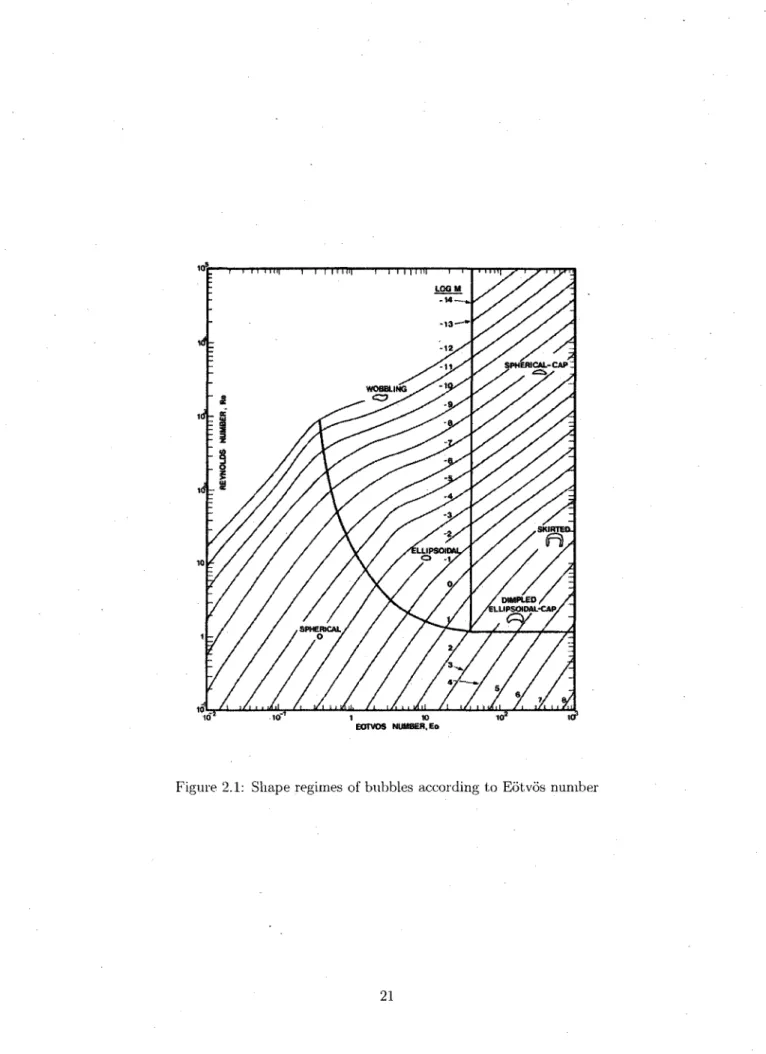
2.1 Shape regimes of bubbles according to Eotvos number 21

5.1 Bubble breakup illustration (a) Luo and Svendsen [55], (b) Martinez-Bazan

etal. [12] 58 5.2 Bubble coalescence in turbulent flow - 63

6.1 Control volume for finite volume discretization 70

6.2 Face interpolation 73 6.3 Decomposition of the face area vector due to non-orthogonality using the

'over-relaxed' approach. . . . 76 6.4 P I S O solution procedure 83

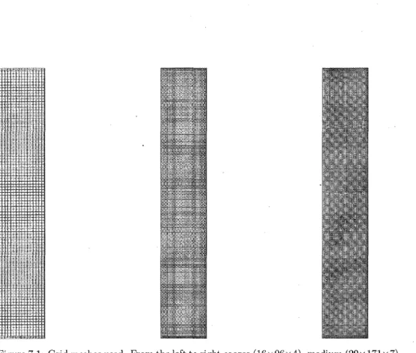
7.1 Grid meshes used. From the left to right coarse (16 x 96 x 4), medium (29 x

171 x 7), fine (40 x 240 x 10) : 88 7.2 Gas hold-up [-•-] mesh refinement tests in the case of Ud,s = 0.14 cm-Is and

H/W = 2.25. Coarse (left), medium (center), fine (right). . -. 90

7.3 Gas velocity [m/s] mesh refinement tests in the case of [/,;,, = 0.14 cm./s and

(18)

7.4 Liquid velocity [m/s] mesh refinement tests in the case of Uds = 0.14 cm,/ s

and H/W = 2.25. Coarse (left), medium (center), fine (right) 91 7.5 Kinetic energy [TO2/*2] mesh refinement tests in the ease of Ufa = 0.14 cm/s

and 77/VF = 2.25 . Coarse (left), medium (center), fine (right) 91 7.6 Dissipation rate [???2/s-i] mesh refinement tests in the case of Ufa — 0.14 cm/s ,

and H/W = 2.25. Coarse (left), medium (center), fine (right) 92 7.7 Turbulent viscosity [m?/s] mesh refinement tests in the case of Ufa =

0.14 cm/s and H/W = 2.25. Coarse (left), medium (center), fine (right). . . . 92 7.8 Turbulent intensity [m/s] mesh refinement tests in the case of Ufa =

.0.14 cm/s and H/W = 2.25. Coarse (left), medium (center), fine (right). . . . 93 7.9 Gas volume fraction [—] mesh refinement tests in the case of Ufa = 0.14 cm/s

and H/W = 4.5. Coarse (left), medium (center), fine (right). . 93 7.10 Gas velocity [m/s] mesh refinement tests in the case of Ufa = 0.14 cm/s and

H/W = 4.5. Coarse (left), medium (center), fine (right) 94

7.11 Liquid velocity [m/s] mesh refinement tests in the case of Ufa = 0.14 cm/s and H/W = 4.5. Coarse (left), medium (center), fine (right) . 94 7.12 Kinetic energy [m"/s~] mesh refinement tests in the case of Ufa = 0.14 cm/s

and H/W = 4.5. Coarse (left), medium (center), fine (right) 95 7.13 Dissipation rate [m"/,s3] mesh refinement tests in the case of Ud,a = 0.14 cm/s

and H/W = 4.5 (HL = 0.90 m). Coarse (left), medium (center), fine (right). . 95

7.14 Turbulent viscosity [m2/.s'J mesh refinement tests in the ease of Ufa =

0.14 cm/s and H/W = 4.5. Coarse (left), medium (center), fine (right). . . . 96 7.15 Turbulent intensity [m/s] mesh refinement tests in the case of Uj.,s =

0.14 cm/s and H/W = 4.5. Coarse (left), medium (center), fine (right). . . . 96

(19)

7.17 Euler-Euler simulation at H/W = 2.25 m, UdjS = 0.73 cin/s for Y = 0.37 m

from the b o t t o m 98

7.18 E-E simulation at H/W = 4.5. U,i,s = 0.14 c m / s (a) and Ud<s = 0.73 c m / s

(b) for Y = 0.675 m 100 7.19 Qualitative comparison of bubbles behavior between experimental results (a)

and present model (b). Conditions are H/W = 2.25. U,i.s — 0.14 cm/s 107 7.20 Qualitative comparison of gas volume fraction between experimental results

(a) and present model (b). Conditions are H/W = 4.5, Ud^ = 0.73 cm/s. . . 108

7.21 E-E simulation at H/W = 2.25, Ud>H = 0.14 cm/s for Y = 0.37 rn 109

7.22 E-E simulation at 11/D = 4.5. Ud.s = 0.14 cm/s (left) and Ud,a = 0.73 cm/s

(right) for Y.= 0.675 m 109

7.23 E-E simulation at H/W = 2.25, Ud<s = 0.14 cm/s for Y = 0.37 m 110

7.24 E-E simulation at H/W = 4.5. UdtS = 0.14 cm/s (left) and f/rf,s = 0.73 cm/s

(right) for F = 0.675 rn 110

7.25 E-E simulation at H/W = 2.25, Ud,s = 0.14 cm,/s for Y = 0.37 m I l l

7.26 E-E simulation at H/W = 4.5, UdiS = 0.14 cm/s (a) and t/rd>s = 0.73 cm/s

(b) for y == 0.37 m I l l

7.27 E-E simulation at H/W = 2.25, Ud>ll = 0.14 CTT7./S for Y = 0.37 m 112

7.28 E-E simulation at # / W = 4,5. [/d,3 = 0.14 cm/s (left) and K,,., = 0.73 ( i n / s

(right) for y = 0.675 m 112 7.29 P I S O solution procedure coupled with P B E and M R F technique 114

7.30 Rectangular laboratory-scale bubble column (right) and perforated section

inlet (left) 116 7.31 Predicted Sauter mean diameter using D Q M O M and t h e method of classes

(20)

7.32 Predicted Sauter mean diameter using DQMOM and 7, 15, 25 different classes

(from left to right). In this case of H/W ='4.5 and Ud,s = 0.14 crn/s 120

7.33 Liquid velocity (left) and gas hold-up (right) profiles using the present model.

H / W = 2.25, Ud.,a =0.14 cm/s for Y = 37 cm from the bottom 121

7.34 Gas hold-up (right) profiles using the present model. H/W = 4.5, Ua.s =

0.14 crn/s for Y = 37 cm from the bottom 121 7.35 Sauter mean diameter profiles using the present model. H/W = 2.25, U,i,s =

0.14 cm/s (left) and H/W = 4 . 5 , t/,y,s =0.14 c?ri/.s (right) 122

7.36 Bubble size distribution using DQMOM in time t = 20s and position of (0.1 x

0.37 x 0.025)m , 123 7.37 Bubble size distribution using DQMOM in time t = 40s and position of (0.1 x

0.37 x 0.025)m ' , 123 7.38 Bubble size distribution using DQMOM in time t = 60s and position of (0.1 x

0.37 x 0.025)™ 124 7.39 Bubble size distribution using-DQMOM in time t = 80s and position of (0.1 x

0.37 x 0.025)rn 124 7.40 Bubble size distribution using CM (7 classes) in time t — 60s and position of

(0.1 x 0.37 x 0.025)m 125 7.41 Bubble size distribution using CM (15 classes) in time t = 60s and position

of (0.1 x 0.37 x 0.025)???, 126 7.42 Solution domain used. The model is solved on the discretized geometry. . . . 129

7.43 Structured mesh grid used in the present model 130 7.44 Contours of Sauter mean diameter at the mid plane (z=0) using DQMOM

(left) and C M (right). The values of ^32 are between 1 and 6 mm (blue to

(21)

7.45 Identification of different loops and radial, positions by Alves 1126| 134 7.46 Predicted gas hold-up using DQMOM and CM (r = 2.4 cm) 135 7.47 Predicted gas hold-up using DQMOM and CM (r = 7.7 cm) 136 7.48 Predicted gas hold-up using DQMOM and CM (r = 13.1 cm) 137 7.49 Predicted bubble diameter using DQMOM as a function of position along

liquid circulation loop 1 138 7.50 Predicted bubble diameter using DQMOM as a function of position along

liquid circulation loop 4 141 7.53 Airlift reactor structured mesh grid 143

7.54 Geometry used in the present model. Airlift bioreactor (left) and gas diffusing

of Fisher brand (right) 146 7.55 Identification of different positions used in airlift bioreactor 148

7.56 Contour of gas hold-up using C M (left) and DQMOM (right) 150 7.57 Gas velocity profiles using C M (left) and DQMOM (right) 151 7.58 Liquid velocity profiles using C M (left) and D Q M O M (right) 152 7.59 Contour of Sauter mean diameter d32 using C M (left) and D Q M O M (right). 153

7.60 Predicted Sauter mean diameter using D Q M O M and CM as a function of

(22)

7.61 Predicted Sauter mean diameter using D Q M O M and C M as a function of

X-position (position 2) 155 7.62 Predicted Sauter mean diameter using D Q M O M and C M as a function of

X-position (position 3) 156 7.63 Predicted mass transfer coefficient ki,a using D Q M O M and C M as a

func-tion of X-posifunc-tion (posifunc-tion 1) 157 7.64 Predicted mass transfer coefficient kj^a using D Q M O M and C M as a

func-tion of X-posifunc-tion (posifunc-tion 2) 158 7.65 Predicted mass transfer coefficient kj^a using DQMOM and CM as a

func-tion of X-posifunc-tion (posifunc-tion3) 159 7.66 Computational time requirement comparison between D Q M O M and CM

(case of bubble column with coarse grid). . 161 7.67 Computational time requirement comparison between D Q M O M and CM

(case of stirred-tank reactor). 162 7.68 Computational time requirement comparison between D Q M O M and CM

(case of airlift reactor) 163

A.l Overview of O'penFOAM structure 172

A.2 The paraFoam window 1.77 A.3 Toolbars in ParaView 178

(23)

List of Tables

3.1 Coefficients used iti the different A; — f models. NC : not considered, T.C :

Tomiyama correlation . . . 31 3.2 Multiplier term used in the two-equation model of turbulence 34

3.3 Numerical boundary conditions applied in this study 39

4.1 Values of weighting function used in Gaussian quadrature integration 50

7.1 Percentage difference of gas hold-up values between model and experimental

measurement of Buwa et al. [135] 102 7.2 Percentage difference of liquid velocity values between model and experimental

measurement of Buwa et al. [135] 102 7.3 Different closures used in bubble column modeling. NC: not considered, C:

considered, B.I.T. : bubble induced turbulence 104 7.4 Values of s and the corresponding classes used with CM 118

7.5 Transport properties 128 7.6 Informations about grid mesh 147

(24)

(25)

Nomenclature

R o m a n S y m b o l s

Symbol Description Units

a interfacial area m2

A surface face rrfi Ad multiplier term used in the two-equation model of turbulence —

AD multiplier term used in the drag force s~~l

bfak) breakup frequency function s"1

C/ friction coefficient kg/mPs3

Ci lift coefficient, dimensionless — Ct turbulence coefficient, dimensionless — Cvm virtual mass coefficient, dimensionless —

C,t k — e constant (; 0.09), dimensionless —

Vt^BiT Bubble induced turbulence coefficient, dimensionless —

d bubble diameter m D reactor diameter m f friction factor — fi bubble volume fraction of group of size i, —

fj bubble volume fraction of group of size j , —

F force vetor N

g acceleration vector due to gravity . rn/s2

II reactor heigh (bubble column) m I unit tensor, dimensionless —

(26)

K exchange coefficient kg/rn Nb number of nodes used in DQMOM method —

ICL mass transfer coefficient m/s

P pressure Pa p(v,Vk) probability function, dimensionless —

S source term

t time , s

U average velocity m/s

U^, velocity of phase 9? m/s

Ur relative velocity m/s

W reactor width m

Greek S y m b o l s

Symbol Description Units a Volume fraction, dimensionless —

• fi Dimensionless coefficient used for Ct model —

A Difference — e Turbulent kinetic energy dissipation rate m2/.s3

//, Dynamic viscosity ky/ms

v Kinematic viscosity m-"/s

p Density kg/nr" a Surface tension N/rn

F,; Break-up frequency of bubbles of size group i s_ 1

7,; Fraction reassigned to nearby classes pivot —

0 angle between U,i and Ur rad

(27)

D i m e n s i o n l e s s N u m b e r s

Symbol Description Definition

F i < Cd Drag coefficient Co Eo Re St Eotvos number Reynolds number Stokes number W e b e r t i n m h e r d • S " ' gApd2 a PrVrd fJ-c Pdd2Ur l%p,.ucL PcdU?

(28)

S u b s c r i p t s & S u p e r s c r i p t s Symbol Description c continuous phase d dispersed phase ip phases index eff effective

(k) first moment order, k = 0, ..,2Nb - 1 t turbulent D drag / lift vm virtual mass r relative i interface dis dispersed in inlet s superficial h hydrolic

(29)

Chapter 1 Introduction

1.1 Background

Bubbly flow regime in the gas-liqwid systems has a very important role in the modern chemi-cal industry for a wide variety of applications including for example bubble'columns, stirred-tank in bio-reactors, rotary gas injection to clean liquid aluminum and air-lift reactors. The optimal design and development of these apparatus rely on the ability to predict the com-plex gas-liquid flow. This can be accomplished by measurements or numerical modelling of the multiphase model equations, known as Computational Fluid Dynamics CFD, and by a combination of the two approaches taking advantage of the strengths of both. The goal of this work is to develop a model which accounts for the coupling of several phenomena such as bubble coalescence and breakage, bubble size distribution and mass transfer. Based on the Computational Fluid Dynamics (CFD) and the opensource CFD library OpenFOAM, we are able to develop new mathematical models including complex flow behavior while maintaining good numerical stability. CFD has been used namely to describe adequately systems as complex as the production of nanoparticles in plasma reactors but its use for

(30)

the multiphase flows of gas-liquid flows encountered in chemical reactors presents different challenges that have been only recently addressed fully. During the last few years, GFD has become an indispensable predicting tool for several engineering, scientific and current life applications. Nevertheless, the use of readily usable commercial CFD software is still far from routine, and for research applications is often very limited. In fact, they are often limited to well-defined applications, so one can not add or modify physical models to suit researchers needs. The use of open source software, such as OpenFOAM, allowed us to de-velop without the constraints of a commercial package, but of course at the expense of a much more involved work in the numerical model itself. At the end, the choice of the CFD platform was between the apparent ease of a commercial package (which is limited in terms of flexibility of the mathematical modelling), and the much more intense work of numerical modelling in an open-source package which involves a total control over all the mathematical an numerical models. At the end, the use of OpenFOAM proved to be a very good choice, combining very good numerical performance with an understanding of all the steps involved in the model from the differential equations set-up to the final report.

The modelling of multiphase flows with the presence of turbulence due to a generally very high agitation is still a tremendous challenge. This task requires both intense material and human resources [39] and it is usually necessary to modify and to adapt the physical and chemical laws according" to the specific application. In most cases, the developed model represents those flows with a certain degree of accuracy, from a numerical point of view. From the literature, it is seen that solutions for these problems are progressing very fast but with some limitations (neglecting of certain forces, geometry different from reality, laboratory scale, numerical methods less eflicient,etc.)- Until now, there are few studies related to the problem of bubbly flows taking into account the bubble coalescence and break-up. These phenomena are due to the strong turbulence created by agitation, or the high inlet gas flows.

(31)

CFD methods, when they can be applied to a system, can provide data otherwise not ac-cessible by traditional experimental techniques in a short time and often for low costs. For this reason, its use in designing multiphase reactors has increased in the last two decades along with the computer power availability. However, CFD is not experimental-free! Ex-perimental validation and correlations are required for the closure of the multiphase model equations. Generally, the formal mathematical modelling of multiphase models uses two approaches. In the first, the bubble and liquid phases are considered as continuous phases, the phases occupying each' a fraction of the volume, thus introducing the concept of volume fraction. This technique, where a set of Eulerian conservation equations is written for each phase is named the Eulerian-Eulerian method. The second method considers only the liquid phase as continuous and the bubble's movements in the liquid are described through a set of Lagrangian trajectory equations. This is the Eulerian-Lagrangian method. In the present study the first method is used, since it is well known that it is better suited for high volume fractions of bubbles encountered locally in the bubble columns. The bubbles and liquid phases are related through interaction forces that are described as drag, lift and virtual mass forces. These interphase forces are formulated, in the mathematical model, as source terms in the momentum conservation equations. The formulation of these terms is relatively straightforward but their inclusion in the numerical algorithm often results in significant difficulties in convergence and stability. Among the authors who introduced these terms in the modeling of bubble columns [49; 133; 103; 134], Many authors also neglected the lift force [17; 95; 96; 44]. However, it has been shown that the lift force has a significant effect on the flow and void fraction fields of the columns j 103: 80; 16|. A few authors used empirical formulations of the lift force coefficient, C/, but mostly it has been assumed a constant value, from 0 to 0.5. Recent studies on bubble columns have been aimed at a better understanding and a more appropriate formulation of the interphase forces [136; 3; 106; 133; 21; 134].

(32)

com-parison with the measurements data of |134; 135; 18]. The other interphase forces, the drag and virtual mass contributions, have been studied in depth by |104; 40; 102]. In the present work, the drag coefficient is also determined using the Tomiyama correlation, which is only a function of the Eotvos number. Virtual mass can be conceptually represented as the change in kinetic energy due to the acceleration of the bubbles. Sato and Sekoguchi f 130] introduced the notion of "Bubble Induced Turbulence", a concept which takes into account the turbu-lence induced by the rotation of bubbles. The present, work aims at the validation of the developed turbulence model and to apply it in the context of population balance modelling (PBM). A study of the current state of the art in the scientific literature on multiphase How modelling reveals that largely, the models do not consider the influence of the dispersed phase and the influence of the gas-liquid interface on turbulence, as well as the turbulence induced by the rotation of the bubbles. In the present work we review many of the different formulations of these terms available in the literature, and proceed to a full integration of the validated terms in the standard k — e model and the population balance equation, using the available published experimental data. The validation of these studies has been made using different gas-liquid systems (bubble columns, air-lift reactors and bio-reactors) [44; 45; 102|. The numerical solution of the developed mathematical model is made using the open source CFD package OpenFOAM (Field Operation And Manipulation) library. OpenFOAM uses advanced numerical methods and formal programming that can be used to represent the mathematical models in a form very close to the natural formulation.

1.2 Problem statement

The main objective of the current research project is to develop a mathematical model that represents the contribution of the turbulence and population balance on the multiphase flows. The problem of turbulence modelling in multiphase flows is studied and outlined in

(33)

the chapter 4. On the other hand, the population balance equation is implemented in the code to taking into account the bubble size distribution function. This model can help to predict the gas-liquid dynamics in the presence of several phenomena in gas-liquid systems. The new open source software OpenFOAM is used for the solution of the model's nonlinear equation set. OpenFOAM presents several advantages; in particular, it provides complete access to the formulation of the mathematical models. Overall, the benefit expected by this study is to improve the efficiency of the processes that can be modelled using the present two-phase How models. This improvement could have an impact on productivity, quality, flexibility .(optimal design of chemical process).

1.3 Objectives

The scientific and technical objectives of this project are the development, validation and application of mathematical models for several multiphase flows applications. The devel-oped model here includes some fundamental aspects and it is broad enough to be applied in industrial applications such as thermal plasma processing, bio-reactors, bubble columns, water treatment, stirred-tank reactors, polymerization and liquid aluminum purification us-ing rotary gas injection process.

This thesis involves the following scientific axes and technical applications: 1. Development of a mathematical model to be used in bubbly flows.

2. Integration of the population balance equation and their solution by an efficient and robust technique; the Direct Quadrature Method of Moments (DQMOM).

3. Modelling of bubble coalescence and break-up phenomena.

4. Validation of the developed model with measurements for three different applications: 4.1 Bubble columns

(34)

4.3 Air-lift bioreactor

5. Prediction of the mass transfer coefficient and Sauter mean diameter in bubbly flow regime

1.4 Present contribution

This study involves a contribution to the Computational Fluid Dynamics field as follows: 1- Development of new combination of physical models extending the standard k — e model of turbulence. A full integration of source terms that represent the dispersed phase and gas-liquid interfaces on multiphase flows are included. The turbulence force induced by the rotational movement of bubbles and the drift velocity are considered.

2- Population balance equation and the use of new resolution techniques such as the direct quadrature method of moments "DQMOM".

3- Modelling of bubble coalescence and breakage using several physical models. 4- Mesh grid dependence study.

1.5 Thesis outline

Chapter 1 is a general introduction to the problem statement and objectives of this work followed by some contributions to complex system modelling.

Chapter 2 presents the mathematical equations describing the Newtonian Multiphase Fluid Flow, the different physical approaches and some of the more relevant physical models in this area.

Chapter 3: A brief definition .of the turbulence modelling is presented. The most popular two-equations models of turbulence are explained and detailed.

(35)

Chapter 4: The population balance equation is introduced. Different solution techniques are highlighted in this section. In our project, the results of modelling are integrated, tested and validated with other numerical models and correlations obtained through experimentation. Chapter 5 is devoted to the various mechanisms of bubble coalescence and break-up. The coupling between CFD and these phenomena is also discussed and developed.

Chapter 6 presents the numerical solution procedure. Spatial and time discretization are also outlined and detailed.

Finally, Chapters 7 and 8 are dedicated to the presentation of results, discussion and con-clusion.

(36)

Chapter 2 Multiphase flow modelling

2.1 Introduction

In this Chapter, a typical multiphase flow system is described. Firstly, governing equations are stated along with basic turbulence and inter-phase mom.entum, exchange modelling. Then, the numerical solution procedure is discussed. The test cases chosen for this purpose are the hydrodynamic behaviour in a rectangular bubble column at differentmesh grid and slirred-tank reactor with double turbine.

In the chemical process industry, complex multiphase flow such as gas-liquid systems are often encountered. In the past, a large number of authors have devoted a considerable amount of effort to formulate field equations. The most important characteristic of a, multiphase flow-is the exflow-istence of an interface separating the continuous and dflow-ispersed phases. The various transfer mechanisms between phases and between a two-phase mixture and a surrounding wall strongly depend upon the two-phase flow regime. The two-phase flows are generally classified into three-flow regimes: the separated, transitional and dispersed flows. In this thesis, we will focus on only dispersed flows because of their most frequent occurrence in the

(37)

modern chemical industry.

In this chapter we look at two mathematical descriptions of two-phase flow. The first ex-amined, is the Lagrangian approach which tracks each discrete particle separately with its trajectory being governed by its own equation of motion within the continuous phase. The second, is the Eulerian approach, treats the phases as inter-penetrating continua and models each phase by averaging the microscopic equations of motion.

2.1.1 Lagrangian A p p r o a c h e s

In the Lagrangian approach, the individual particles of the dispersed phase or a statistical sample thereof, are tracked through (he flow domain. The conservation equation of momen-tum for each of the particles is expressed in a co-ordinate frame of reference which follows the trajectory. The resulting equation, which describes the motion of the particle in the continuous medium, relates the rate of change of the particle's velocity to the sum of forces acting upon it:

, , ^ = £ F (2.1, where

Urf is the velocity of dispersed phase

pd is the dispersed phase density

F is the individual forces acting on the particles

The commonly accepted Lagrangian equation governing the motion of a particle at low Reynolds numbers reads [116|:

(38)

dt v pc Dt 2 pc \ Dt Dt. '

+ ¥!?M£±

['" Vp&Lzgldr + g(1 1 Bl) (

f<» d dt{Vd - Uc) , prf 2

.

2

)

where

- <i/d^ Derivative with respect to time following the moving particle. - D/Dt Total acceleration of the continuous phase as seen by the particle. - \J,i Velocity of dispersed phase particle.

- Uc. Velocity of continuous phase.

- g Gravity.

- nip Mass of particle.

- rrif Mass of fluid displaced by the particle = mP{pc/p(i)

- r Particle radius.

- F Q Drag force exerted on particle due to relative motion. - pc Dynamic viscosity of the continuous phase.

- pa Density of the dispersed phase. - pc Density of the continuous phase.

- tp Particle response time.

Another significant advantage of the Lagrangian approach is that since there is one equation of motion for each particle, it is relatively easy to account for a distribution of particle sizes. Also, in gas-liquid and liquid-liquid systems, where the bubbles or droplets can break up into two or more smaller fragments or coalesce into a larger entity, the Lagrangian approach can be easily applied. The strategy of a Lagrangian analysis of two-phase flow is usually to follow a sufficient number of particles individually through the flow domain by solving the above equation for each one. The calculated trajectories of the particles are then used to obtain

(39)

information regarding the average nature of the flow, such as the dispersion coefficient, the local volume fraction or the local velocity.

The coupling between the continuous phase and the dispersed phase is often tackled in the solution procedure by using a two-step iterative approach. Here, the continuous phase flow is determined at a, particular instant in time after which the motion and position of the in-dividual dispersed phase elements are updated according to the newly calculated continuous phase flow. The exchange of momentum between phases is evaluated between steps so that it can be included as sources or sinks in the subsequently solved equations for the other phase. The sequence is repeated until sufficient data on the motion of the dispersed phase has been gathered by Kralj fllj. However, problems arise with the Lagrangian approach when the system of interest contains many particles. The first problem is that since there is one equation of motion for each particle the problem may become computationally too large to allow the trajectory of every particle to be calculated. Many particle trajectories are required in order to obtain meaningful information on the average nature of the flow. For example, a typical stirred-tank reactor (say with a volume of 6 m3) with particles of 1 mm

in diameter at a volume fraction of 1% contains approximately 108 particles. In such cases, a

representative sample of particles trajectories are calculated and the overall flow properties inferred from these. Secondly, for high to moderate phase fractions, the increased coupling between the particles and the continuous phase can introduce numerical stability problems [11|.

2.1.2 Eulerian Methods in Two Phase Flow

In the Eulerian approach, both the continuous and dispersed phases are described using Eulerian conservation equations written in fixed co-ordinates. Each phase is treated as a continuous medium, each inter-penetrating the other, and is represented by macroscopic

(40)

conservation equations, one set for each phase, which are valid throughout the entire flow domain. This approach is commonly known as the 'Two-Fluid' approach, or when more than two phases are considered, the 'Multi-Fluid' approach Ishii [77].

The two-fluid conservation equations are derived from the fundamental conservation equa-tions for mass, momentum and energy which govern the behaviour of each phase and which are valid within each phase up to the interface between the phases: the familiar Navier-Stokes equations. The two-fluid conservation equations are obtained by applying a. suitable averaging procedure to the entire two-phase system. The resulting mathematical form of the two-fluid equations is similar to the single-phase Navier-Stokes equations but contain extra terms which account for the transfer of mass and momentum between phases. In princi-ple, the two-fluid approach is applicable to the entire range of flow regimes encountered in multi-phase flows, including the separated, dispersed and intermediate regimes. The physi-cal character of the extra inter-phase mass and momentum transfer terms depends heavily on the exact nature of the flow, but the Eulerian approach is only limited by the ability to accurately model these terms, and is not inherently limited to dispersed systems. The generality of this approach comes at a cost, however, and it's main disadvantage is the dif-ficulty in prescribing suitable inter-phase models for the flow regime under consideration. The identification of relevant inter-phase forces, such as drag, lift or virtual mass, is not as obvious as in the Lagrangian approach where each is represented by its own term and modelling the effects of many particles in averaged form can add considerable complexity to the modelling process. Similarly, the derivation of models which are applicable to flows which are between well defined regimes, or where the regime varies in different parts of the flow, can be extremely complex and the physical understanding of these situations may not be sufficiently well developed until now. However, the two-lluid approach is frequently more efficient than the Lagrangian approach, since individual dispersed phase elements are not tracked and the calculations are not restricted to the transient case.

(41)

The two- fluid equations for both phases are discretised using the same computational mesh and are often solved using similar techniques to those employed for single-phase How but suitably extended to account for the coupled nature of the flow. Importantly, this approach allows the numerical problems arising from the coupling between phases to be more easily handled. For these reasons, the two-fluid approach has proven to be popular in the study of two-phase systems and has been adopted as the basis for the present work.

2.2 Governing equations

2.2.1 Continuity equation

To solve the multiphase model equations, discrete approaches need to be used. The time and spatial domain is subdivided in a finite elements. The most common and widely used discretization techniques are finite difference, finite volume and finite element methods [124; 67]. In the present work the finite volume method is used for solving non-linear equations system. A general local continuity equation of the quantity ip can be written as:

^ K ) + V - ( avU „ ) = 0 (2.3)

Where ov is the volume fraction of a phase ip and Uv is the velocity magnitude of phase tp.

In the Eulerian frame, the following relation must be respected:

] T aV = 1.0 (2.4)

In order to solve the problem of boundedness, Spalding |25] suggested that Eqn. (2.3) should be solved for a<i and its counterpart for ac, the solutions should then be recombined:

(42)

The new phase fraction field akd will be bounded by zero and one only if ad and ac are both

larger than zero and it follows that appropriate differencing is essential.

Weller [61] re-arranged the phase continuity Eqn. (2.3) so that all terms are in conservative form and a.a can be bounded at both ends, as follows:

^ + V • (Uad) + V • ( Urad( l - ad)) = 0 (2.6)

Where U = ad\3d + arJJc and Ur = Vd - Uc.

2.2.2 Momentum equation

In absence of mass transfer between phases and for incompressible fluids in the steady-state

regime, the local conservation equation of momentum is:

- ( ^ U ^ + V . t ^ U y U ^ + V . t a ^ v V U , , ) = -a^Vp + V.{TV) + av~g +"F +RV (2.7)

Where TV represent the Reynolds stress tensor for the continuous phase defined as:

r > - ! # ' ( V Uv + V . Vv - | / V . U„ ) + pk (2.8)

and Ry, represent the Coriolis and centrifugal forces applied in the rotating reference of frames (MR..F) and is written as follow:

Rv = -2av/)¥,N^J x. U ^ - Q ^ ^ N ^ x (N^ x r v) (2.9)

Here N represent the rotating velocity (RPM) and T* is the position vector (m). ;/£ is —> —>

the effective kinematic viscosity of phase <p. Uv and F are respectively the velocity field of

(43)

2.2.3 Interfacial m o m e n t u m e x c h a n g e e q u a t i o n s

In the present work the drag and the lift forces developed by Tomiyama et al. [4] are used to determine the interfacial momentum exchange. In the Eulerian-Eulerian approach used here, and at high volume fraction (>10%) we consider the dispersed phase as a continuous phase using the same momentum and continuity equations applied for the continuous phase. Hence, the instantaneous inter-phase momentum exchange is determined by assembling the forces acting on the dispersed bubbles. The main contributions are drag, lift, virtual mass, and the Basset forces. In this section, the exchange terms are written as components of these different contributions:

F = FD + Ft + F vm (2.10)

The Drag Force

The relative motion between a submerged body and the surrounding fluid gives rise to the so-called drag force. It is a resistance of a particle in a fluid environment such as water or air. For spherical dispersed phase particles we have Rusche [56|:

FD = Az>Ur (2.11)

Where

3adCD -f

A B = — ^ — |U.r| (2.12)

Here d is the bubble or particle diameter, Ur is the mean relative velocity (U^ — Uc) . The

drag coefficient Co depends on the characteristics of the flow surrounding the body and is a function of the Eotvos number for the case of bubbles. In the present work, for the. drag coefficient C'D the particle drag model of Tomiyama is chosen, which gives good results for

(44)

large bubbles (> 5 mm) and is defined as folio i w :

_ 8 E o ( l - ^ ) 1

° 3 £?2/3Eo + 16(1 - E2)Ei F{Ef K ' ' '

Where Eo is the Eotvos number defined as:

E o = = ^ ^ : • (2.14)

a

The Eotvos parameter is a dimensionless number and it can be used to characterize the shape of bubbles (see Fig. 2.1) or drops moving in a surrounding fluid. Eotvos number may be regarded as proportional to buoyancy force divided by surface tension force.

Here, g and a are respectively the gravity and surface tension. 1 l + 0.163Eo0-757 and (2.15) Eod = ^ (2.16) and

F{E)

_

Sin

-K^W)

E

-Evr^w

{2n}

(45)

EOTVOS NUMBER, E<>

(46)

The Lift Force

The lift force F / describes the lateral force experienced by a particle subjected to a shearing flow field or due to.the rotation of the particle itself. It is important for gas-liquid systems in which regions of high shear exist and it can have a large effect on phase distribution. The lift fore is defined as suggested by Drew |23| and |22|:

F z = adq UPx ( V x Uc) (2.18)

Here Ci represent the lift coefficient which is calculated using the Tomiyama correlation as follows:

jmin\0.288tanh(0.121Re),f{Eod)} Eod < 4

\f(Eod) 4 sC Eod < 10.7

whe: re

f(Eod) = 0.105(Eod)3 QM59(Eod)2 0.0204.Eorf + 0.474 (2.20)

The Virtual Mass Force

By definition, the virtual mass force can be understood by considering the change in kinetic energy of fluid surrounding an accelerating bubble. The effect of virtual mass force is much larger for a bubble in liquid than for a drop in gas due to the higher liquid density surrounding the bubble. The virtual mass coefficient Cvm is often set to 0.5 for rigid spherical particles

in the literature Carrica et al. [98]. For low phase fraction Fw„ is given as:

F,; m = a( ;C „ ^ — ^ J (2.21)

Where -~ denotes the substantive derivative which is delined as:

(47)

The Basset Force

The Basset force represents the influence of the time dependent development of the boundary layer on the particle surface in accelerating flows. In essence, it takes into account the fact that the drag on the particle depends on the previous history of the particle motion. The Basset force is given by:

F , 4 ^ ^ ( | U

r f

U

C

|

W7

£= (2.23)

in gas-liquid flows, the Basset force is very small when compared to the drag force and is usually neglected.

2.2.4 Interfacial c l o s u r e s u m m a r y

Collecting the models for the various interfacial forces described above and substituting them into Eqn. (2.10) we have

F = | ^ £ u r | U r | + adCtVr x (V x Uc) + acCvm(^± - BgLfj (2.24)

In this work, two values of 0.25 and 0.5 for the virtual mass coefficient are used in the comparison with the experimental data.

(48)

Chapter 3 Turbulence modelling

Turbulence modeling is one of three key elements in computational fluid dynamics (CFD), in particular when one is interested in industrial processes Wilcox J26J. The other key elements are the grid generation and numerical algorithms development. By definition, a mathematical model of turbulence is one that approximates the real physical behaviour of turbulent flows. As examples of turbulence motion, flow in the wake of a cylinder, bubble columns, stirred reactors,...etc. Really most of all flows of practical engineering situations are turbulent.

3.1 Introduction

Most fluid flows occurring in nature are turbulent. Turbulence can be described as a state of continuous instability in the flow, where it is still possible to separate the fluctuations from the mean flow properties. It is characterized by irregularity in the flow, increased diffusivity and energy dissipation Tetmekes and Luinley [57]. Turbulent flows are always three-dimensional and time dependent, even if the boundary conditions of the flow do not change in time. The range of scales in such flows is very large, from the smallest turbulent

(49)

eddies characterized by Kolmogorov microscales, to the flow features comparable with the size of the geometry. A comprehensive review of simulation techniques for turbulent flows can be found in Ferziger and Peric [69] works. A brief overview of the modelling techniques will be given here.

There are several possible approaches to the simulation of turbulent Hows. The first, Direct Numerical Simulation (DNS) (|130; 129; 115; 87|) numerically integrates the governing equations over the whole range of turbulent scales. The requirements on mesh resolution and time-step size put very high demands on the computer resources, rendering it unsuitable for engineering applications. The second approach is generally known as Large Eddy Simulation (LES). In order to separate different length scales in a turbulent flow field, a spatial filter is applied. Large scale structures that can be resolved by the numerical method on a given mesh are called the super-grid scales. The influence of all other (sub-grid) scales to the super-grid behaviour is modelled. The rationale behind this principle lies in the fact that the small scales of turbulence are more homogeneous and isotropic and therefore easier to model. As the mesh gets finer, the number of scales that require modelling becomes smaller, thus approaching the Direct Numerical Simulation. Examples of this approach can be found in [73; 65; 138]. In the present study, the above approaches cited here (DNS, LES, R A N S ) are presented here briefly as follow:

• Direct Numerical Simulation (DNS): it is not a model, Navier-Stokes Equations are computed in their most general form meaning that the complete spec-trum of involved frequencies and length scales are solved. This approach is only feasible at current time for Low Reynolds number flows, due to limitation on computer resources, and used mainly as validation test for other approaches or as a help in understanding turbulence physics.

(50)

mainly in the largest scales, this model reduces the range of interest only to the biggest vor-tices. It employs, in fact, a time dependent three dimensional computation of the large-eddy structure and a model for the small scales. It basically consists in filtering in space the Navier-Stokes Equations with a high-pass filter, resolving for scales that actually are the energy-containing scales and modelling dissipation subrange behaviour. LES is becoming more and more popular in the CFD community, particular complexities in treating bound-ary conditions and the need for wide computer resources still limit the use to simple geome-tries and specific areas of interest in which turbulence modelling is more than fundamental (turbulent combustion, wake effects, chemical reactions).

• Reynolds Averaged Navier Stokes (RANS): Navier-Stokes Equa-tions are averaged in time on a period long enough to contain also lowest frequency oscillation. The unsteady behaviour of the turbulent flows is completely neglected, turbulence become a steady phenomenon simply considering the effects of fluctuations onto the mean flow. At the state of art RANS simulations are the standard for flows involving heat transfer of industrial interest. In fact unsteady phenomena result in being determinant for such simulations. Be-cause of its ease of implementation and the speed in solving, supported by a good accuracy in modelling mean flows, one can reasonably believe that this approach will be used for many years to come.

3.2 History of turbulence modelling

The earliest attempts to constructing a mathematical model of turbulence flows goes back to Boussinesq [62| works which introduced the concept of the so-called eddy viscosity. In the nineteenth century, Prandtl (1925) introduced the mixing length which formed the basis of all turbulence modeling research for the next twenty years. In 1945's, Prandtl postulated a model in which the eddy viscosity depends upon the kinetic energy of the turbulent

(51)

fluctu-ations, k. He proposed a partial-differential equation approximating t h e exact equation for

k. This model is thus called one-equation model of turbulence.

Kolmogorov (1942) introduced the first complete model of turbulence. In addition to having an equation for k, he introduced a second parameter u t h a t he referred to as "the rate of dissipation of energy in unit volume and time". This model is thus termed a two-equation model of turbulence. It went with virtually no applications for the next 25 years because of the unavailability of computers to solve its nonlinear differential equations.

3 . 2 . 1 o n e - e q u a t i o n m o d e l s o f t u r b u l e n c e

P r a n d t l (1945) postulated t h a t t h e dissipation assumes t h e following form Wilcox [26|:

e.~/fc3 / 2/i (3.1)

Introducing a closure coefficient Ck, the dissipation is:

e = Ckki/'2/l (3.2)

Thus, P r a n d t l ' s one-equation model is as follows:

dk T T dk dUi „ fc3/2 d u t. .,

at

+

^aTj =

^

~

CD~ +

aT, K"

+

">*)]

(^)

where T.^ is the Reynolds-Stress Tensor, if we assume the Boussinesq approximation, t h e

Reynolds-Stress is given by:

2

Tij = ZvrSij - -kSij (3.4)

Here, SV, is t h e strain-rate tensor. We can define t h e kinematic: eddy viscosity as follows:

i / = fc1/2/ = CD— (3.5)

T h e one-equation model is not, by far, a universal turbulence model. Therefore the devel-opment of more general models is necessary.

(52)

3.2.2 Two-equation models of turbulence

Turbulence modelling for two-phase flows has been reviewed recently by several authors [36; 16; 34: 53]. As in a single-phase flow turbulence modelling, second-order closure models, which solves transport equations for each component of the Reynolds stresses, constitutes the highest level of closure currently feasible for practical applications. So far, only two authors [28; 80| developed two-phase Reynolds stress turbulence models, whereas the majority of authors invoke the Boussinesq [62[ hypothesis and model the turbulent stress-strain relation analogous to the constitutive relation of a viscous fluid, e.g. [27; 123; 5; 131; 42; 103; 92; 50]. The turbulent viscosity is then related to the fluid's turbulent kinetic energy k and its dissipation rate e, which axe governed by their own transport equations.

We limit our discussion to the more commonly used k — e models. In fact, a wide variety of k — e models exists, the most noteworthy being the standard k — e model by Jones and Launder [72]. Before building and analyzing the structure of the transport equation for .turbulent kinetic energy k and turbulent kinetic energy dissipation e, a general overview common to all k — e models is needed, in order to understand how k and e are related to the wanted scalar / / .

First the turbulent length scale It is computed locally as:

h = C„ (3.6)

e

and second, following the definition of length, scale, one obtains:

IH = CljPk^% = CliP— (3.7)

(53)

3.2.3 T h e s t a n d a r d k - e m o d e l

The most popular two-equation turbulence model is the k — e model. The central paper for this model is that published by Jones and Launder [72| which is, in the turbulence modelling community, well known as the standard k — e model of turbulence. The idea in this model is to derive the exact equation of e and to find suitable closure approximations for other parameters. Tims, the standard k — e is as follows:

Turbulent viscosity k2

,/ = a

(3.8) Kinetic energy dk dk dt + "dxj dVj d 13 dx,j ' dx-j (v + u'lok)-dk Dissipation rate de TT de e . .dU-i, „ e2 d

m

+V3

dx-

= c

^k

TlJ

l^--

c

^

+

dx-dXj\ (v + S/cTc) .de dx.j

Closure coefficients and auxiliary relations:

Ce,i = 1.44, Ct-2 = 1.92, C^ = 0.09, ak = 1.0, at = 1.3

3.2.4 T h e M n d d e e t al. (1999) closure t e r m s for k - e m o d e l

(3.9)

(3.10)

Following the work of Robert and Oliver |49|, the two-equations k e model has been modified to the following formulation:

and

- | Lck\ + V • (a,XJ(A = V • (aAVfc ) + nfc + Wk

y (ace\ + V • (acUce) = V • L % e ) + IT, + U\

(3.11)

(54)

Where n^ and TTr denote the ordinary one-phase production and dissipation terms defined

as follow

Uk=acG (3.13)

and

ns= ac| ( ( 7 i G - C 7 2 e ) (3.14)

Here, G stands for the production of turbulent kinetic energy and is defined as:

G = 2i4ff (vUc • deu(VUc + (VU( :)T)) (3.15)

Where dev represents the deviatory component defined as:

devT = T - l(tr{T)) (3.16)

T is a second rank tensor and tr is the trace of this tensor..

The effective viscosity of the continuous phase is calculated from v'l- = vc + i/ where / /

is given by the Eqn. (3.8). The values of Cfl, C'i, C2, c> and ot are unchanged from the

(55)

Table 3.1: Coefficients used in the different k — t models. NC : not considered, T.C Tomiyaina correlation Constants Fluent OpenFOAM This work

c,

0.09 0.09 0.09 Cx 1.44 1.44 1.44 C-h 1.92 1.92 1.92

c

3 1.2 NC 1.2 Ck 1.0 1.0 1.0 <?t 1.3 1.3 1.3

c

t NC NC

c

t CjhBlT NC NC 0.6

From the equations (3.11) and (3.12) ITj. and II*'includes the effect of the interfaces on the turbulent kinetic energy and the dissipation rate respectively. According to Bel F'Dhila and Simonin [103], the IT^ term is formulated as:

14 = , P* .adFD[ < U;..Urf >d -2k + UA.i / t. Ur] (3.17)

where < Uc. Ud >d represent the covariance defined by the Eqn. (3.30).

The IIJ is modelled according to Elghobashi and Abou-Arab [12-5 j:

n : = cZ-n% (3.18) Where C3 is constant of the standard model of turbulence (see table 3.1) and F^ is the drag

force density coefficient given by:

Fd = {^^L) (3.19)

Tp

and Udrift is the drift velocity used to correct the relative velocity as follows:

Ur = (Ud Uc) Udrlft (3.20)

As mentioned, the drift velocity accounts for the dispersion of the particles due to transport by turbulent fluid motion and is calculated by Robert, and Oliver [49|:

Udrift — ~Dc,d ' VCrd VOfc

ad ac

(56)

where DL(i d is the fluid-bubble turbulent dispersion tensor and is expressed as:

, D\,d = 3 < J < U^u< i >2 (3.22)

In Robert and Oliver [49] works, the turbulence of the dispersed phase is treated using three . time scales: the characteristic time of turbulent eddies T^, the characteristic time of particles

entrainment by the fluid motion r*d and the characteristic time of the fluid turbulence viewed

by the bubbles T* d. The last three time scales are given by:

2L"e (3.23) and F __ 1 (Pd , r * d V Pc _t Ok T14 = ^\1 + C3C (3.24) (3.25)

Here, C,r is the ratio between the characteristic time of the turbulent eddies and the

charac-teristic transit time, r^d, required for the bubbles to cross the large eddies:

Cr |UJ

id

wwm

(3.26)

The parameter Cp is defined as:

Op = 1 . 8 - 1.35cos2(0) (3.27)

with

cos{9) UdUr (3.28)

l|U(J|| • ||Ur|

the turbulent kinetic energy k^ of the dispersed phase and the covariance < X}'c.X3d >c; are

given by:

~b2 +r)r

k,i = k

(57)

and b + rir l+Vr\ <Vc.Ud>d=2k\ 1 + CA i/pc + C

In this model, only the effect of the interfaces on the turbulence terms are included.

(3.30)

with 7ir = TIJT^ and b = +' ^ (CA = 0.5).

3.2.5 T h e R u s c h e (2002) closure t e r m s for k — t m o d e l

As mentionned, most two-phase turbulence models of dispersed flows are based on a single-phase turbulence model for the continuous single-phase. The presence of the dispersed single-phase is accounted for by additional terms. Recently, Tabor |50| outlined a more elaborate, four-equation model where separate k — e systems are assembled for each phase. This model requires additional closure and more effort is needed to finalize the coupling terms. However, in the work of Rusche |5G|, the two-fluid turbulence model extended by Gosman et al. |5| is adopted. It consists of the standard k — e model of Jones and Launder [72] with the effect of the dispersed phase on the turbulence, while the model of Robert and Oliver [49] presented above deals with the effect of the interface. The two-equations k — e are then written as:

f r»„k \ 4 V • [ nJl.k. \ X7 • i

-j - (ack\ + V • (acXJck J - V • (^—-Vifc J = Uk - ae + Ufs (3.31)

£ (ajj + V • (acVce\ - V • f ~ " V e ) = Ue + I l f (3.32)

The additional two-phase source terms are:

.Jdts _ 2kadAd(Ct - 1) , A,y(/' Vad —

n*a = ° , n ' ' + - ^ - - ^ • UT. (3.33)

Pc PcP a-c

ldts 2C-AeadAd(Ct - 1)

(58)

Table 3.2: Multiplier term used in the two-equation model of turbulence Multiplier term

Here, the drag multiplier term Af;, which depends on the inter-phase momentum transfer,

is defined in Table 3.2. In this model, the presence of dispersed phase is accounted for by additional source terms, which are related to that of the continuous phase through a turbulence response coefficient, C't, (see [56; 5; 111; 6; 2|) in which the correlation proposed by Issa and Oliveira |112| is adopted:

C = 3+l% Jt 1 + ,8,. + 2Pd/Pc

Where: (3t = ^ ^ ; R e , = H ^ . L = C}ll, v' =

/ icR e t i'c a

Where u,i and i/c are respectively the the kinematic viscosity of dispersed and continuous

phase. Re,, is the Reynolds number based on the eddy length scale Lc.

Gosman et al. [5] Weller [611

(59)

Here the C,ia and C,ic terms are defined as follow Weller [61]:

C = ( 2 4 ^ A i , ) ( l + 0 . 1 5 ( ^ ^ r8 7) (3.36)

and

Cdc = (24z/d/dc)(l + 0 . 1 5 ( ^ l )a 6 8 7) (3.37)

Finally, the Reynolds stresses are obtained from the Boussinesq hypothesis |62|, which models the turbulent stress-strain relation analogous to the constitutive relation of a. viscous lluid. It is given by:

K" = - ^ " ( V U y + V U J - | l V • U„) + | l ^ (3.38)

3.2.6 N e w c o m b i n a t i o n of k — e m o d e l s (present c o n t r i b u t i o n )

In order to improve the modelling of the two-phase flows studied in the present thesis, we extend the models proposed by Robert and Oliver [491 and Rusche |56| described above and combine them to take into account both the effect of the interface and the dispersed phase effects. The proposed model is solved and validated through a comparison with the measurements of Buwa and Ranade [134] and Pfleger et al. [18) available in the literature. The following resulting transport equations of turbulence, still based on an extension of the standard k — c model incorporate the effect of the interfaces and the dispersed phase on the turbulence:

~(ack) + V • (U,.&) = V • ( ar— V f c ) + arG ~~ are + arITk + a(Hfs (3.39)

at <Jk

and

4 ( «ce ) + V • (Uce) = V • ( «C^ - V e ) + *cUdG - C2c) + aJTt + ««JI*8 (3.40)

All source terms IIJ., II*, II*S and Ilf's presented in this model are expressed by the Eqns.