On challenges in training recurrent neural networks

Universit´e de Montr´eal

On Challenges in Training Recurrent Neural Networks

par

Sarath Chandar Anbil Parthipan

D´epartement d’informatique et de recherche op´erationnelle Facult´e des arts et des sciences

Th`ese pr´esent´ee `a la Facult´e des arts et des sciences en vue de l’obtention du grade de Philosophiæ Doctor (Ph.D.)

en informatique

Composition du jury

Pr´esident-rapporteur: Jian-Yun Nie Directeur de recherche: Yoshua Bengio

Co-directeur: Hugo Larochelle Membre du jury: Pascal Vincent Examinateur externe: Alex Graves

Résumé

Dans un probl`eme de pr´ediction `a multiples pas discrets, la pr´ediction `a chaque instant peut d´ependre de l’entr´ee `a n’importe quel moment dans un pass´e lointain. Mod´eliser une telle d´ependance `a long terme est un des probl`emes fondamentaux en apprentissage automatique. En th´eorie, les R´eseaux de Neurones R´ecurrents (RNN) peuvent mod´eliser toute d´ependance `a long terme. En pratique, puisque la magnitude des gradients peut croˆıtre ou d´ecroˆıtre exponentiellement avec la dur´ee de la s´equence, les RNNs ne peuvent mod´eliser que les d´ependances `a court terme. Cette th`ese explore ce probl`eme dans les r´eseaux de neurones r´ecurrents et propose de nouvelles solutions pour celui-ci.

Le chapitre 3 explore l’id´ee d’utiliser une m´emoire externe pour stocker les ´etats cach´es d’un r´eseau `a M´emoire Long et Court Terme (LSTM). En rendant l’op´eration d’´ecriture et de lecture de la m´emoire externe discr`ete, l’architecture propos´ee r´eduit le taux de d´ecroissance des gradients dans un LSTM. Ces op´erations discr`etes permettent ´egalement au r´eseau de cr´eer des connexions dynamiques sur de longs intervalles de temps. Le chapitre 4 tente de caract´eriser cette d´ecroissance des gradients dans un r´eseau de neurones r´ecurrent et propose une nouvelle architecture r´ecurrente qui, grˆace `a sa conception, r´eduit ce probl`eme. L’Unit´e R´ecurrente Non-saturante (NRUs) propos´ee n’a pas de fonction d’activation Non-saturante et utilise la mise `a jour additive de cellules au lieu de la mise `a jour multiplicative.

Le chapitre 5 discute des d´efis de l’utilisation de r´eseaux de neurones r´ecurrents dans un contexte d’apprentissage continuel, o`u de nouvelles tˆaches apparaissent au fur et `a mesure. Les d´ependances dans l’apprentissage continuel ne sont pas seulement contenues dans une tˆache, mais sont aussi pr´esentes entre les tˆaches. Ce chapitre discute de deux probl`emes fondamentaux dans l’apprentissage continuel: (i) l’oubli catastrophique d’anciennes tˆaches et (ii) la capacit´e de saturation du r´eseau. De plus, une solution est propos´ee pour r´egler ces deux probl`emes lors de l’entraˆınement d’un r´eseau de neurones r´ecurrent.

Mots cl´es: R´eseaux de Neurones R´ecurrents, D´ependances `a long terme, Unit´e R´ecurrente Non-saturante, R´eseaux de Neurones `a M´emoire Augment´ee, Machine Neuronale de Turing, LSTMs, connexions dynamiques, apprentissage continuel, oubli catastrophique, capacit´e de saturation.

Summary

In a multi-step prediction problem, the prediction at each time step can depend on the input at any of the previous time steps far in the past. Modelling such long-term dependencies is one of the fundamental problems in machine learning. In theory, Recurrent Neural Networks (RNNs) can model any long-term dependency. In practice, they can only model short-term dependencies due to the problem of vanishing and exploding gradients. This thesis explores the problem of vanishing gradient in recurrent neural networks and proposes novel solutions for the same.

Chapter 3 explores the idea of using external memory to store the hidden states of a Long Short Term Memory (LSTM) network. By making the read and write operations of the external memory discrete, the proposed architecture reduces the rate of gradients vanishing in an LSTM. These discrete operations also enable the network to create dynamic skip connections across time. Chapter 4 attempts to characterize all the sources of vanishing gradients in a recurrent neural network and proposes a new recurrent architecture which has significantly better gradient flow than state-of-the-art recurrent architectures. The proposed Non-saturating Recurrent Units (NRUs) have no saturating activation functions and use additive cell updates instead of multiplicative cell updates.

Chapter 5 discusses the challenges of using recurrent neural networks in the context of lifelong learning. In the lifelong learning setting, the network is expected to learn a series of tasks over its lifetime. The dependencies in lifelong learning are not just within a task, but also across the tasks. This chapter discusses the two fundamental problems in lifelong learning: (i) catastrophic forgetting of old tasks, and (ii) network capacity saturation. Further, it proposes a solution to solve both these problems while training a recurrent neural network.

Keywords: Recurrent Neural Networks, Long-term Dependencies, Non-saturating Recurrent Units, Memory Augmented Neural Networks, Neural Turing Machines, LSTMs, skip connections, lifelong learning, catastrophic forgetting, capacity satu-ration.

Contents

2.1.3 Conditional Language Modeling . . . 6

2.1.4 Sequential Decision Making . . . 7

2.2 Vanilla Recurrent Neural Networks . . . 7

2.2.1 Limitations of Feedforward Neural Networks . . . 7

2.2.2 Recurrent Neural Networks . . . 8

2.3 Problem of vanishing and exploding gradients . . . 10

2.4 Long Short-Term Memory (LSTM) Networks. . . 11

2.4.1 Forget gate initialization . . . 13

2.5 Other gated architectures . . . 14

2.6 Orthogonal RNNs . . . 16

2.7 Unitary RNNs . . . 17

2.8 Statistical Recurrent Units . . . 17

2.9 Memory Augmented Neural Networks . . . 18

2.9.1 Neural Turing Machines . . . 19

2.10 Normalization methods . . . 24

Chapter 3: LSTMs with Wormhole Connections . . . 27

3.1 Introduction . . . 27

3.2 TARDIS: A Memory Augmented Neural Network . . . 28

3.2.1 Model Outline . . . 29

3.2.2 Addressing mechanism . . . 30

3.2.3 TARDIS Controller . . . 31

3.2.4 Micro-states and Long-term Dependencies . . . 32

3.3 Training TARDIS . . . 34

3.3.1 Using REINFORCE . . . 35

3.3.2 Using Gumbel Softmax . . . 37

3.4 Gradient Flow through the External Memory . . . 37

3.5 On the Length of the Paths Through the Wormhole Connections. . 41

3.6 On Generalization over the Longer Sequences . . . 43

3.7 Experiments . . . 45

3.7.1 Character-level Language Modeling on PTB . . . 45

3.7.2 Sequential Stroke Multi-digit MNIST task . . . 45

3.7.3 NTM Tasks . . . 48

3.7.4 Stanford Natural Language Inference . . . 49

3.8 Conclusion . . . 49

Chapter 4: Non-saturating Recurrent Units. . . 51

4.1 Introduction . . . 51

4.2 Non-saturating Recurrent Units . . . 52

4.2.1 Discussion . . . 54

4.3 Experiments . . . 54

4.3.1 Copying Memory Task . . . 55

4.3.2 Denoising Task . . . 60

4.3.3 Character Level Language Modelling . . . 61

4.3.4 Permuted Sequential MNIST . . . 62

4.3.5 Model Analysis . . . 62

4.4 Conclusion . . . 65

Chapter 5: On Training Recurrent Neural Networks for Lifelong Learning . . . 67

5.1 Introduction . . . 67

5.2 Related Work . . . 70

5.2.1 Catastrophic Forgetting . . . 70

5.2.2 Capacity Saturation and Model Expansion . . . 72

5.3 Tasks and Benchmark . . . 74

5.3.2 Associative Recall Task. . . 75

5.3.3 Sequential Stroke MNIST Task . . . 75

5.3.4 Benchmark . . . 76

5.3.5 Rationale for using curriculum style setup . . . 78

5.4 Model . . . 79

5.4.1 Gradient Episodic Memory (GEM) . . . 79

5.4.2 Net2Net . . . 82

5.4.3 Extending Net2Net for RNNs . . . 83

5.4.4 Unified Model . . . 85

5.4.5 Analysis of the computational and memory cost of the pro-posed model . . . 86 5.5 Experiments . . . 87 5.5.1 Models . . . 87 5.5.2 Hyper Parameters. . . 88 5.5.3 Results. . . 88 5.6 Conclusion . . . 92

Chapter 6: Discussions and Future Work . . . 93

6.1 Summary of Contributions . . . 93

6.2 Future Directions . . . 94

6.2.1 Better Recurrent Architectures . . . 94

6.2.2 Exploding gradients . . . 94

6.2.3 Do we really need recurrent architectures? . . . 94

6.2.4 Recurrent Neural Networks for Reinforcement Learning . . . 95

6.2.5 Reinforcement Learning for Recurrent Neural Networks . . . 95

6.3 Conclusion . . . 96

List of Figures

2.1 A vanilla Recurrent Neural Network. Biases are not shown in the illustration. . . 9

2.2 RNN unrolled across the time steps. An unrolled RNN can be consid-ered as a feed-forward neural network with weights W , U , V shared across every layer.. . . 9

2.3 Long Short-Term Memory (LSTM) Network. . . 12

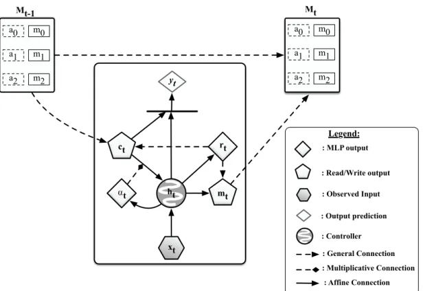
3.1 At each time step, controller takes xt, the memory cell that has been

read rt and the hidden state of the previous timestep ht 1. Then,

it generates ↵t which controls the contribution of the rt into the

internal dynamics of the new controller’s state ht (We omit the t

in this visualization). Once the memory Mt becomes full, discrete

addressing weights wr

t is generated by the controller which will be

used to both read from and write into the memory. To predict the target yt, the model will have to use both ht and rt. . . 33

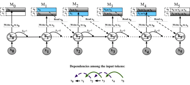
3.2 TARDIS’s controller can learn to represent the dependencies among the input tokens by choosing which cells to read and write and creat-ing wormhole connections. xt represents the input to the controller

at timestep t and the ht is the hidden state of the controller RNN. 34

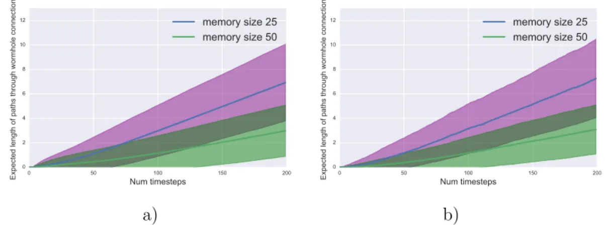
3.3 In these figures we visualized the expected path length in the memory cells for a sequence of length 200, memory size 50 with 100 simula-tions. a) shows the results for TARDIS and b) shows the simulation for uMANN with uniformly random read and write heads. . . 41

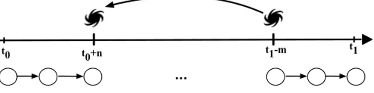
3.4 Assuming that the prediction at t1 depends on the t0, a wormhole

connection can shorten the path by creating a connection from t1

m to t0 + n. A wormhole connection may not directly create a

connection from t1 to t0, but it can create shorter paths which the

gradients can flow without vanishing. In this figure, we consider the case where a wormhole connection is created from t1 m to t0+ n.

3.5 We have run simulations for TARDIS, MANN with uniform read and write mechanisms (uMANN) and MANN with uniform read and write head is fixed with a heuristic (urMANN). In our simulations, we assume that there is a dependency from timestep 50 to 5. We run 200 simulations for each one of them with di↵erent memory sizes for each model. In plot a) we show the results for the expected length of the shortest path from timestep 50 to 5. In the plots, as the size of the memory gets larger for both models, the length of the shortest path decreases dramatically. In plot b), we show the expected length of the shortest path travelled outside the wormhole connections with respect to di↵erent memory sizes. TARDIS seems to use the memory more efficiently compared to other models in particular when the size of the memory is small by creating shorter paths. . . 44

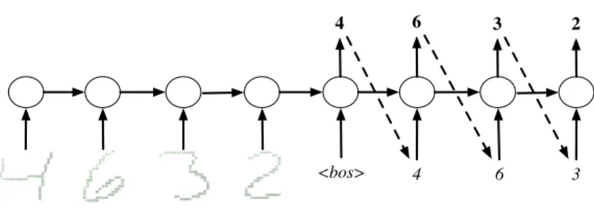
3.6 An illustration of the sequential MNIST strokes task with multiple digits. The network is first provided with the sequence of strokes information for each MNIST digits (location information) as input, during the prediction the network tries to predict the MNIST digits that it has just seen. When the model tries to predict, the predictions from the previous time steps are fed back into the network. For the first time step, the model receives a special <bos> token which is fed into the model in the first time step when the prediction starts. 47

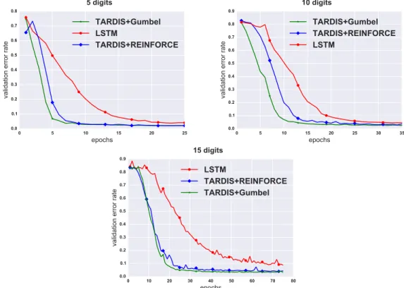
3.7 Learning curves for LSTM and TARDIS for sequential stroke multi-digit MNIST task with 5, 10, and 15 multi-digits respectively. . . 48

4.1 Copying memory task for T = 100 (in top) and T = 200 (in bottom). Cross-entropy for random baseline : 0.17 and 0.09 for T=100 and T=200 respectively. . . 56

4.2 Change in the content of the NRU memory vector for the copying memory task with T=100. We see that the network has learnt to use the memory in the first 10 time steps to store the sequence. Then it does not access the memory until it sees the marker. Then it starts accessing the memory to generate the sequence. . . 58

4.3 Variable Copying memory task for T = 100 (in left) and T = 200 (in right). . . 59

4.4 Comparison of top-3 models w.r.t the number of the steps to con-verge for di↵erent tasks. NRU concon-verges significantly faster than JANET and LSTM-chrono. . . 60

4.5 Denoising task for T = 100. . . 61

4.7 Gradient norm comparison with JANET and LSTM-chrono across the training steps. We observe significantly higher gradient norms for NRU during the initial stages compared to JANET or LSTM-chrono. As expected, NRU’s gradient norms decline after about 25k steps since the model has converged. . . 64

4.8 E↵ect of varying the number of heads (left), memory size (middle), and hidden state size (right) in psMNIST task.. . . 65

5.1 Per-level accuracy on previous tasks, current task, and future tasks for a 128 dimensional LSTM trained in the SSMNIST task distri-bution by using the curriculum. The model heavily overfits to the sequence length. . . 79

5.2 Current Task Accuracy for the di↵erent models on the three “task distributions”(Copy, Associative Recall, and SSMNIST respectively). On the x-axis, we plot the index of the task on which the model is training currently and on the y-axis, we plot the accuracy of the model on that task. Higher curves have higher current task accuracy and curves extending more have completed more tasks. For all the three “task distributions”, our proposed small-Lstm-Gem-Net2Net model clears either more levels or same number of levels as the large-Lstm-Gem model. Before the blue dotted line, the proposed model is of much smaller capacity (hidden size of 128) as compare to other two models which have a larger hidden size (256). Hence the larger models have better accuracy initially. Capacity expansion technique allows our proposed model to clear more tasks than it would have cleared otherwise. . . 89

5.3 Previous Task Accuracy for the di↵erent models on the three task distributions (Copy, Associative Recall, and SSMNIST respectively). Di↵erent bars represent di↵erent models and on the y-axis, we plot the average previous task accuracy (averaged for all the tasks that the model learned). Higher bars have better accuracy on the previ-ously seen tasks and are more robust to catastrophic forgetting. For all the three task distributions, the proposed models are very close in performance to the large-Lstm-Gem models and much better than the large-Lstm models. . . 89

5.4 Future Task Accuracy for the di↵erent models on the three task distributions (Copy, Associative Recall, and SSMNIST respectively). Di↵erent bars represent di↵erent models and on the y-axis, we plot the average future task accuracy (averaged for all the tasks that the model learned). Higher bars have better accuracy on the previously unseen tasks and are more beneficial for achieving knowledge transfer to future tasks. Even though the proposed model does not have any component for specifically generalizing to the future tasks, we expect the proposed model to generalize at least as well as the large-Lstm-Gem model and comparable to large-Lstm. Interestingly, our model outperforms the large-Lstm model for Copy task and is always better than (or as good as) the large-Lstm-Gem model. . . 90

5.5 Accuracy of the di↵erent models (small-Lstm-Gem-Net2Net, large-Lstm-Gem and large-Lstm respectively) as they are trained and eval-uated on di↵erent tasks for the Copy and the SSMNIST task dis-tributions. On the x-axis, we show the task on which the model is trained and on the y-axis, we show the accuracy corresponding to the di↵erent tasks on which the model is evaluated. We observe that for the large-Lstm model, the high accuracy values are concen-trated along the diagonal which indicates that the model does not perform well on the previous task. In the case of both small-Lstm-Gem-Net2Net and large-Lstm-Gem models, the high values are in the lower diagonal region indicating that the two models are quite resilient to catastrophic forgetting. . . 91

List of Tables

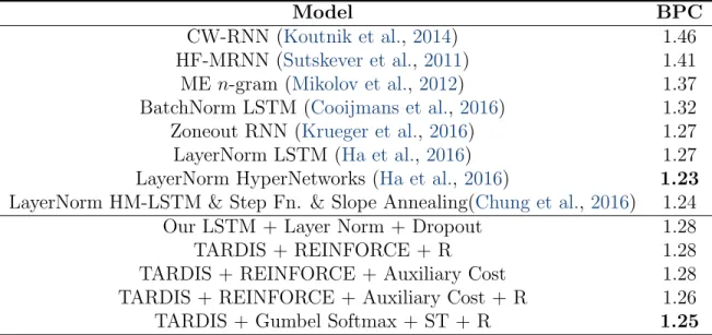
3.1 Character-level language modelling results on Penn TreeBank Dataset. TARDIS with Gumbel Softmax and straight-through (ST) estimator performs better than REINFORCE and it performs competitively compared to the SOTA on this task. ”+ R” notifies the use of RE-SET gates ↵ and . . . 46

3.2 Per-digit based test error in sequential stroke multi-digit MNIST task with 5,10, and 15 digits. . . 48

3.3 In this table, we consider a model to be successful on copy or as-sociative recall if its validation cost (binary cross-entropy) is lower than 0.02 over the sequences of maximum length seen during the training. We set the threshold to 0.02 to determine whether a model is successful on a task as in (Gulcehre et al., 2016). . . 49

3.4 Comparisons of di↵erent baselines on SNLI Task. . . 50

4.1 Number of tasks where the models are in top-1 and top-2. Maximum of 7 tasks. Note that there are ties between models for some tasks so the column for top-1 performance would not sum up to 7. . . 55

4.2 Bits Per Character (BPC) and Accuracy in test set for character level language modelling in PTB. . . 62

4.3 Validation and test set accuracy for psMNIST task. . . 63

5.1 Comparison of di↵erent models in terms of the desirable properties they fulfill. . . 74

List of Abbreviations

BPTT Backpropagation Through Time

CIFAR Canadian Institute for Advanced Research DL Deep Learning

D-NTM Dynamic Neural Turing Machine EUNN Efficient Unitary Neural Network

EURNN Efficient Unitary Recurrent Neural Network EWC Elastic Weight Consolidation

FFT Fast Fourier Transform GEM Gradient Episodic Memory

GORU Gated Orthogonal Recurrent Unit GRU Gated Recurrent Unit

HAT Hard Attention Target HMM Hidden Markov Model

iCaRL Incremental Classifier and Representation Learning IMM Incremental Moment Matching

JANET Just Another NETwork KL divergence Kullback-Leibler divergence

LRU Least Recently Used LSTM Long Short Term Memory

LwF Learning without Forgetting

ML Machine Learning MLP Multi-Layer Perceptron

MNIST Mixed National Institute of Standards and Technology NMC Nearest Mean Classifier

NOP No Operation

NRU Non-saturating Recurrent Unit NTM Neural Turing Machine

psMNIST Permuted Sequential MNIST PTB Penn Tree Bank

QP Quadratic Programming

REINFORCE REward Increment = Nonnegativev Factor times O↵set Reinforcement times Characteristic Eligibility

ReLU Rectified Linear Unit RNN Recurrent Neural Network

SNLI Stanford Natural Language Inference SOTA State-of-the-art

SRU Statistical Recurrent Unit SSMNIST Sequential Stroke MNIST

To my mother Premasundari. For all the sacrifices that she has made! She is the reason I’m where I am today!!

Acknowledgments

August 2014. I was visiting Hugo Larochelle’s lab at the University of Sher-brooke. Hugo and I were discussing my options for a PhD. “If you want to do a Ph.D. in Deep Learning, you have to do it with Yoshua,” Hugo had said. I applied only to the University of Montreal and I got an o↵er to do my Ph.D. with Yoshua Bengio and Hugo Larochelle. I accepted the o↵er and the next four years were a wonderful journey. If I have to go back and redo my Ph.D., I would do it exactly in the same way!

I should start my acknowledgements by thanking Hugo Larochelle. I know Hugo since NeurIPS 2013. Not only did he show me the right path to do my Ph.D. with Yoshua, but he also agreed to co-supervise me. In the last four years, Hugo has been my adviser, mentor, teacher, and well-wisher. Even though this thesis does not include any of my joint work with Hugo, this thesis is not possible without his advice and mentoring.

My next thanks are to Yoshua Bengio. Yoshua gave me the independence to do my research. However, he was always there every time I got stuck and our discussions always helped me progress. He always encouraged me to do good science and not run after publications. Yoshua and Hugo together are the best combination of advisers one could ask for!

I would like to thank my primary collaborators without whom this thesis is not possible: Caglar Gulcehre, Chinnadhurai Sankar, and Shagun Sodhani. Chapters 3, 4, and 5 in this thesis are joint work with Caglar, Chinna, and Shagun respectively. I am grateful to be part of Mila, which is a very vibrant and dynamic research lab that one can think of. I would like to thank the following Mila faculty members for several technical and career-related discussions over the last four years: Lau-rent Charlin, Aaron Courville, Will Hamilton, Simon Lacoste-Julien, Guillaume Lajoie, Roland Memisevic, Ioannis Mitliagkas, Chris Pal, Prakash Panangaden, Liam Paull, Joelle Pineau, Doina Precup, Alain Tapp, Pascal Vincent, Guillaume Rabusseau. I would like to thank Dzmitry Bahdanau, Harm de Vries, William Fedus, Prasanna Parthasarathi, Iulian Vlad Serban, Chiheb Trabelsi, and Eugene Vorontsov for several interesting conversations. I would like to thank my lecoinnoir team for all the fun in the workplace. Special thanks to Laura Ball for keeping our corner green!

I would like to thank the Google Brain Team in Montreal for hosting me as a student research scholar for the last 2 years. I have had several stimulating research discussions with Hugo Larochelle, Marc Bellemare, Laurent Dnih, Ross Goroshin, Danny Tarlow and Shibl Mourad (DeepMind) in the Google office. A special thanks to my manager Natacha Mainville for always making sure that I never had any blocks in my research and work at Google.

I would like to thank everyone who participated in Hugo’s weekly meetings: David Bieber, Liam Fedus, Disha Srivastava, and Danny Tarlow. Despite being on a friday, these meetings were always fun! I would like to thank the following external researchers for several interesting research discussions and career-related advice: Kyunghyun Cho, Orhan Firat, Marlos Machado, Karthik Narasimhan, Siva Reddy. During my Ph.D., I was lucky to mentor Mohammad Amini, Vardhaan Pahuja, Gabriele Prato, Shagun Sodhani, and Nithin Vasishta. I would like to thank all of them for the knowledge that I gained through mentoring them.

In the last seven years of my research, I was extremely lucky to have several good collaborators. Apart from the ones mentioned above, I would like to thank the fol-lowing: Ghulam Ahmed Ansari, Alex Auvolat, Sungjin Ahn, Nolan Bard, Michael Bowling, Neil Burch, Alexandre de Brebisson, Murray Campbell, Mathieu Duches-neau, Vincent Dumoulin, Iain Dunning, Jakob N. Foerster, Jie Fu, Alberto Garcia-Duran, Revanth Gengireddy, Mathieu Germain, Edward Hughes, Samira Kahou, Nan Rosemary Ke, Khimya Ketarpal, Taesup Kim, Marc Lanctot, Stanislas Lauly, Zhouhan Lin, Sridhar Mahadevan, Vincent Michalski, Subhodeep Moitra, Alexan-dre Nguyen, Emilio Parisotto, Prasanna Parthasarathi, Michael Pieper, Olivier Pietquin, Janarthanan Rajendran, Sai Rajeshwar, Vikas Raykar, Subhendu Ron-gali, Amrita Saha, Karthik Sankaranarayanan, Francis Song, Jose M. R. Sotelo, Florian Strub, Dendi Suhubdy, Sandeep Subramanian, Gerry Tesauro, Saizheng Zhang.

I would like to thank Simon Lacoste-Julien for accepting me to TA for his graphical models course for 2 years. In my Ph.D., I also got the opportunity to teach the Machine Learning course at McGill twice. I would like to thank all the 300+ students who took the course. I learned a lot by teaching this course. Special thanks to all my TAs for supporting me to teach such a large scale course.

Throughout my Ph.D., I was fortunate to hold several fellowships and scholar-ships. I was supported by an FQRNT-PBEEE fellowship by the Quebec Govern-ment for the second and third year. I was supported by an IBM Ph.D, fellowship for the fourth and fifth years. I also received the Antidote scholarship for NLP by Druide Informatique. Google also supported my Ph.D. by giving me a student research scholar position which allowed me to work part-time at Google Brain Mon-treal. I would like to thank all these institutions for providing financial support which helped me to do my research. Special thanks to all the sta↵ members at

Mila who made my Ph.D. life much easier: Fr´ed´eric Bastien, Myriam Cote, Joce-lyne Etienne, Mihaela Ilie, Simon Lefrancois, Julie Mongeau, and Linda Peinthiere. I would like to thank my undergrad adviser Susan Elias for introducing me to research, my Master’s adviser Ravindran Balaraman for introducing me to Machine Learning, my long-term collaborator and mentor Mitesh Khapra for introducing me to Deep Learning.

This thesis would not have been possible without the support of my friends and family! I will start by acknowledging my room-mate for the first three years: Chin-nadhuari Sankar. We had technical discussions even while cooking and driving. Our pair-programming in late nights has resulted in several interesting projects includ-ing the NRU (presented in this thesis). Special thanks to Gaurav Isola, Prasanna Parthasarathi, and Shagun Sodhani for being good friends, and well-wishers, and supporting me whenever I face any personal issues. Thanks to Igor Kozlov, Ritesh Kumar, Disha Srivastava, Sandeep Subramaniam, Nithin Vasishta, and Srinivas Venkattaramanujam for all the fun time in Montreal. I would like to thank my long-time friends Praveen Muthukumaran and Nivas Narayanasamy for supporting me through thick and thin. I would like to thank my music teacher Divya Iyer for accommodating my busy research life and teaching me music whenever I find the time. Music, for me, is a soul recharging experience!

Ph.D. is a challenging endeavour. It is the support of my family which encour-aged me to keep going. I would like to thank Sibi Chakravarthi for everything he has done for me. Life would be boring without our silly fights! I also would like to thank Chitra aunty for her support and advice. She always treats me the same way as Sibi. I would like to thank Mamal Amini for all his love and care. Montreal has given me a Ph.D. and a career, but you are the best gift that Montreal gave me. Thank you for being such an awesome friend and brother. Thank you for making sure I go to the gym even if there is a deadline the next day! I would like to thank my sister Parani for her constant support. She always cares for me and encourages me every time I feel down. I would like to thank my wife Sankari for supporting my dreams and understanding every night I was working in front of the desktop (including the night I am writing this acknowledgement section!). Thank you for your love and a↵ection. I would like to thank my mom Premasundari for everything. I am the world for her. This thesis is rightly dedicated to her. Finally, I would like to thank my father Parthipan for everything. He always wanted to see me as a scientist. Now I can finally say that I have achieved your dreams for me dad! You are still living in our memories and I know you will be feeling proud about me right now!

1

Introduction

Designing general-purpose learning algorithms is one of the long-standing goals of artificial intelligence and machine learning. The success of Deep Learning (DL) (LeCun et al.,2015; Goodfellow et al.,2016) demonstrated gradient descent as one such powerful learning algorithm. However, it shifted the attention of the machine learning research community from the search for a general-purpose learning algo-rithm to the search for a general-purpose model architecture. This thesis considers one such general-purpose model architecture class: Recurrent Neural Networks (RNNs). RNNs have become the de-facto models for sequential prediction prob-lems. Variants of RNNs are used in many natural language processing applications like speech recognition (Bahdanau et al., 2016), language modeling (Merity et al.,

2017), machine translation (Wu et al., 2016), and dialogue systems (Serban et al.,

2017). RNNs are also used for sequential decision-making problems (Hausknecht and Stone, 2015).

While RNNs are more suitable for sequential prediction problems, they can also be useful computation models for one-step prediction problems. A one-step predic-tion problem like image classificapredic-tion could still benefit from recurrent reasoning steps over the available information to make better predictions as demonstrated by

Mnih et al. (2014). Thus any improvements to RNNs should have a significant im-pact on the general problem of prediction. This thesis proposes several architectural and algorithmic improvements in training recurrent neural networks.

RNNs, even though a powerful class of model architectures, are difficult to train due to the problem of vanishing and exploding gradients (Hochreiter,1991;Bengio et al.,1994). While training an RNN using gradient descent, gradients could vanish or explode as the length of the sequence increases. While exploding gradients destabilize the training, vanishing gradients prohibit the model from learning long-term dependencies that exist in the data. Learning long-long-term dependencies is one of the central challenges for machine learning. Designing a general-purpose recurrent architecture which has no vanishing or exploding gradients while maintaining all its expressivity remains an open question. The first half of this thesis attempts to answer this question.

Moving away from the single-task setting where one trains a model to perform only one task, the second half of the thesis considers a multi-task lifelong learning

setting. In a lifelong learning setting, the network has to learn a series of tasks rather than just one task. This is beneficial since the network can transfer knowl-edge from one task to another and hence learn new tasks faster than learning them from scratch. However, this comes with additional challenges. When we train an RNN to learn multiple tasks it might forget the previous tasks while learning the new task and hence its performance in previous tasks might degrade. This is known as catastrophic forgetting (McCloskey and Cohen, 1989). Also note that RNNs are finite capacity parametric models. When forced to learn more tasks than its capacity allows, an RNN tends to unlearn previous tasks to free the capacity to learn new tasks. We call this capacity saturation. Note that capacity saturation and catastrophic forgetting are related issues. While capacity saturation leads to catastrophic forgetting, it is not the only source of catastrophic forgetting. Another source is the gradient descent algorithm itself which forces the parameter to move to a di↵erent region in the parameter space to learn the new task better. The thesis attempts to provide solutions to tackle these additional challenges that would arise in a lifelong learning setting.

1.1

Contributions

The key contributions of this thesis are as follows:

— Dynamic skip-connections to avoid vanishing gradients. In a typical recurrent neural network, the state of the network at each time step is a function of the state of the network at previous time step. This creates a linear chain that the gradients has to pass through. We propose a new recurrent architecture called “TARDIS” which learns to create dynamic skip connections to previous time steps so that the gradients can pass directly to a previous time step without passing through all the intermediate time steps. This significantly reduces the rate at which gradients vanish (Chapter 3).

— A recurrent architecture with no vanishing gradients. In this thesis, we propose a new recurrent architecture which does not have any vanishing gradients by construction. We call the architecture “Non-saturating Recur-rent Unit” (NRU) (Chapter 4).

— RNNs for lifelong learning. We study the problem of using RNNs for life-long learning. While most of the existing work on lifelife-long learning focused on catastrophic forgetting, this work highlights that the issue of capacity satura-tion is also important and proposes a hybrid learning algorithm which would tackle both catastrophic forgetting and capacity saturation. Specifically, we

extend the individual solutions for these problems from the feed-forward lit-erature and also merge them to tackle both problems together (Chapter 5). This thesis is based on the following three publications:

1. Caglar Gulcehre, Sarath Chandar, Yoshua Bengio. Memory Augmented Neu-ral Networks with Wormhole Connections. In arXiv, 2017.

— Personal Contributions: The model is inspired from our earlier work (Gulcehre et al., 2016). Caglar came up with the idea of tying the read-ing and writread-ing head. Caglar performed the language model and SNLI experiments. I created the sequential stroke multi-digit MNIST task and performed the benchmark experiments. Caglar and I wrote the paper with significant contributions from Yoshua.

2. Sarath Chandar*, Chinnadhurai Sankar*, Eugene Vorontsov, Samira Ebrahimi Kahou, Yoshua Bengio. Towards Non-saturating Recurrent Units for Mod-elling Long-term Dependencies. Proceedings of AAAI, 2019.

— Personal Contributions: I was looking for alternative solutions for vanishing gradients after the TARDIS project. Yoshua suggested the idea of using a flat memory vector with ReLU based gating in one of our discussions. I developed NRUs based on this suggestion. I designed the experiments and implemented the tasks. Chinnadhurai and I ran most of the experiments. Eugene helped us by running the unitary RNN baselines. I wrote the paper with feedback from all the authors.

3. Shagun Sodhani*, Sarath Chandar*, Yoshua Bengio. Towards Training Re-current Neural Networks for Lifelong Learning. Neural Computation, 2019. — Personal Contributions: The idea of studying the capacity saturation issue in lifelong learning was mine. I also came up with the idea of combining Net2Net with methods that mitigate catastrophic forgetting. I designed the tasks and Shagun ran all the experiments and we both wrote the paper together with feedback from Yoshua.

1.2

Thesis layout

The rest of the thesis is organized as follows. Chapter 2 introduces sequential problems and recurrent neural networks. Chapter 2 also introduces the problem of vanishing and exploding gradients and provides necessary background on state-of-the-art recurrent architectures which aim to solve this problem. Chapter 3 and chapter 4 introduce two di↵erent solutions to solve the vanishing gradient problem: LSTMs with wormhole connections and Non-saturating Recurrent Units respec-tively. Chapter 5 discusses the challenges in training RNNs for lifelong learning

and proposes a solution. Chapter 6 concludes the thesis and outlines future re-search directions.

2

Background

In this chapter, we will provide the necessary background on recurrent neural networks to understand this thesis. We assume that the reader already knows the basics of machine learning, neural networks, gradient descent, and backpropagation. See (Goodfellow et al.,2016) for a relevant textbook.

2.1

Sequential Problems

This thesis focuses on sequential problems and we give the general definition of a sequential problem here.

In a sequential problem, at every time step t, the system receives some input xt

and has to produce some output yt. The number of time steps is a variable and it

can potentially be infinite (in which case the system receives an infinite stream of inputs and produces an infinite stream of outputs). The input xt at any time step

t can be optional and so is the output yt at any time step t. yt at any time step

might be dependent on any of the previous xtor even all of previous xtwhich makes

the problem more challenging than the standard single step prediction problems where the output depends on just the immediately preceding input.

Now we will show several example applications which can be considered in this framework of sequential problems.

2.1.1

Sequence Classification

Given a sequence x1, ..., xT, the task is to predict yT which is the class label of

the sequence. This can be considered in the general sequential problem framework with no output yt at all time steps except for t = T . The sequence is defined as

(x1, ), (x2, ), ..., (xT 1, ), (xT, yT).

Example applications include sentence sentiment classification where given a sequence of words, the task is to predict whether the sentiment of the sentence is positive, negative or neutral.

2.1.2

Language Modeling

Given a sequence of words w1, ..., wT, the goal of language modeling is to model

the probability of seeing this sequence of words or tokens, P (w1, ..., wT). This can

be represented as the conditional probability of the next word given all the previous words: P (w1, ..., wT) = T Y t=1 P (wt|wt 11 ) (2.1)

where wt 1₁ refers to w1, ..., wt 1 and w01 is defined as null. This task can be

posed as a sequential prediction problem where at every time t, given w1, ..., wt 1,

the system predicts wt. The sequence flow for this problem is defined as ( , w1),

(w1, w2), ..., (wT 1, wT). At any point in time t, the system has seen the previous

t 1 words (over t 1 time steps) and hence should be able to model the probability of the t-th word given the previous t 1 words. A system trained with a language modeling objective can be used for unconditional language generation by sampling a word given the sequence of previously sampled words. It may also be used to score a word sequence by P (w1, ..., wT) using equation 2.1.

2.1.3

Conditional Language Modeling

In conditional language modeling, we model the probability of a sequence of words w1, ..., wT given some object o: P (w1, ..., wT|o). The conditioning object o

itself can be a sequence. There are several applications for conditional language modeling.

In question answering, given a question (which is a sequence of words), the sys-tem has to generate the answer (which is another sequence of words). In machine translation, given a sequence of words in one language, the system has to generate another sequence of words in a di↵erent language. In image captioning, given an image (which is a single object), the system has to generate a suitable caption (which is a sequence of words). In dialogue systems, given the previous utterances (each of which is a sequence of sentences), the system has to generate the next utterance (which is a sequence of words). The sequence flow for conditional lan-guage modeling is defined as (o1, ), ..., (oT1, ), ( , w1), ..., ( , wT2) where T1 is 1 for

2.1.4

Sequential Decision Making

In sequential decision making, at any time step t, the agent perceives a state st

and takes an action at. Based on the current state and the action, the agent receives

some reward rt+1and moves to a new state st+1with probability P (st+1|st, at). The

goal of the agent is to find a policy (i.e. which action to take in the given state) such that it can maximize the discounted sum of the rewards, where the future rewards are discounted by some discount factor 2 [0, 1]. The sequence flow in this setting is (_{{ , s}1}, a1), ({r2, s2}, a2), ..., ({rT, sT}, aT). This is the central

problem of Reinforcement Learning.

2.2

Vanilla Recurrent Neural Networks

In this section, we will first show the limitations in using feed-forward networks for sequential problems. Then we will introduce recurrent neural networks as an elegant solution for sequential problems. We assume discrete outputs throughout the discussion (i.e. yt takes a finite set of values). The discussion can be easily

extended to the continuous output setting.

2.2.1

Limitations of Feedforward Neural Networks

Feedforward neural networks are the simplest neural network architectures that take some input x and predict some output y. Consider a sequential problem where at every time step t, the network receives xt and has to predict yt. The typical

architecture of a feedforward one-hidden layer fully-connected neural network is defined as follows:

ht= f (U xt+ b) (2.2)

ot= sof tmax(Vht+ c) (2.3)

where f is some non-linearity function like sigmoid or tanh, and ht is the hidden

state of the network. U is the input to hidden state connection matrix and V is the hidden state to output connection matrix. b and c are the bias vectors for the hidden layer and the output layer respectively. Softmax gives a valid probability distribution over possible values yt can take.

the negative log-likelihood of yt given xt. L = T X t=1 log Pmodel(yt|xt) (2.4)

This loss function can be minimized by using the backpropagation algorithm. This simple model learns to predict yt solely based on xt. Hence, it cannot capture the

dependency of yt with some previous xt0 with t0 < t. In other words, this is a

state-less architecture since it cannot remember previous xt0 while making prediction for

the current yt.

The straightforward extension of this architecture to model the dependencies with previous inputs is to consider previous k inputs while predicting the next output. The architecture of such a network is defined as follows:

ht = f (U1xt+ U2xt 1+ ... + Ukxt k+1+ b) (2.5)

ot = sof tmax(Vht+ c) (2.6)

The loss function in this case is L =

T

X

t=1

log Pmodel(yt|xt, xt 1, ..., xt k+1) (2.7)

While we simulate states in this architecture by explicitly feeding the previous k inputs, this model has limited expressive power in the sense that it can only model the dependencies within the previous k inputs. In addition, the number of parameters of the model grows linearly as the value of k increases. Ideally we would expect to model the dependencies with all the previous inputs and also avoid this linear growth in the number of parameters as the length of the sequence increases.

2.2.2

Recurrent Neural Networks

Recurrent Neural Networks (RNNs) are a family of neural network architectures specialized for processing sequential data. RNNs are similar to feedforward net-works except that the hidden states have a recurrent connection. RNNs can use this hidden state to remember the previous inputs and hence the hidden state at any point of time acts like a summary of the entire history. The typical architecture of a simple, or vanilla RNN is defined as follows:

ht= f (U xt+ W ht 1+ b) (2.8)

where the matrix W corresponds to hidden to hidden connections. The initial hidden state h0 can be initialized to a zero vector or can be learned like other

parameters. Figure 2.1 shows the architecture of this RNN. RNNs when unrolled across time correspond to a feedforward neural network with shared weights in every time step (see Figure2.2). Hence one can learn the parameters of the RNN by using backpropagation in this unrolled network. This is known as backpropagation through time (BPTT). The memory required for BPTT increases linearly with the length of the sequence. Hence we often approximate BPTT with truncated BPTT in which we truncate the backprop after some k time steps.

o_t h_t= f ( ) x_t V W U

Figure 2.1 – A vanilla Recurrent Neural Network. Biases are not shown in the illustration.

o₁ h₁= f ( ) x₁ V W U h₀ o₂ h₂= f ( ) x₂ V W U o₃ h₃= f ( ) x₃ V W U o_t h_t= f ( ) x_t V W U

Figure 2.2 – RNN unrolled across the time steps. An unrolled RNN can be considered as a feed-forward neural network with weights W , U , V shared across every layer.

The loss function in this case could be L =

T

X

t=1

log Pmodel(yt|xt1) (2.10)

RNNs have several nice properties suitable for sequential problems. 1. Prediction for any yt is dependent on all the previous inputs.

2. The number of parameters is independent of the length of the sequences. This is achieved by sharing the same set of parameters across the time steps. 3. RNNs can naturally handle variable length sequences.

2.3

Problem of vanishing and exploding

gradients

Even though RNNs are capable of capturing long term dependencies, they often learn only short term dependencies. This is mainly due to the fact that gradients vanish as the length of the sequence increases. This is known as vanishing gradient problem and has been well studied in the literature (Hochreiter,1991;Bengio et al.,

1994).

Consider an RNN which at each timestep t takes an input xt2 Rdand produces

an output ot2 Ro. The hidden state of the RNN can be written as,

zt= W ht 1+ U xt, (2.11)

ht= f (zt). (2.12)

where W and U are the recurrent and the input weights of the RNN respectively and f (_{·) is a non-linear activation function. Let L =}PT_t=1Lt be the loss function

that the RNN is trying to minimize. Given an input sequence of length T , we can write the derivative of the loss L with respect to parameters ✓ as,

@_L @✓ = X 1t1T @_Lt1 @✓ = X 1t1T X 1t0t1 @_Lt1 @ht1 @ht1 @ht0 @ht0 @✓ . (2.13)

The multiplication of many Jacobians in the form of @ht

@ht 1 to obtain

@h_t1

@h_t0 is the

main reason of the vanishing and the exploding gradients (Pascanu et al., 2013b): @ht1 @ht0 = Y t0<tt1 @ht @ht 1 = Y t0<tt1 diag[f0(zt)]W . (2.14)

Let us assume that the singular values of a matrix M are ordered as, 1(M) 2(M) · · · n(M). Let ↵ be an upper bound on the singular values of W , s.t.

↵ 1(W ), then the norm of the Jacobian will satisfy (Zilly et al.,2016),

|| @ht

@ht 1||  ||W || ||diag[f 0_(z

Pascanu et al. (2013b) showed that for _|| @ht @ht 1||  1( @ht @ht 1)  ⌘, the following inequality holds: || Y t0tt1 @ht @ht 1||  1 Y t0tt1 @ht @ht 1 !  ⌘t1 t0_{. (2.16)} where ↵||f0_(z

t)||  ⌘ for all t. We see that the norm of the product of Jacobians

grows exponentially on t1 t0. Hence, if ⌘ < 1, the norm of the gradients will vanish

exponentially fast. Similarly, if ⌘ > 1, the norm of the gradients may explode exponentially fast. This is the problem of vanishing and exploding gradients in RNNs. While gradient clipping can limit the e↵ect of exploding gradients, vanishing gradients are harder to prevent and so limit the network’s ability to learn long term dependencies.

The second cause of vanishing gradients is the activation function f . If the activation function is a saturating function like a sigmoid or tanh, then its Jacobian diag[f0(zt)] has eigenvalues less than or equal to one, causing the gradient signal to

decay during backpropagation. Long term information may decay when the spectral norm of (W diag[f0_(z

t)]) is less than 1 but this condition is actually necessary in

order to store this information reliably (Bengio et al.,1994;Pascanu et al.,2013b). Designing a recurrent neural network architecture which has no vanishing or exploding gradients is an open question in the RNN literature. While there are certain recurrent architectures which have no vanishing or exploding gradients, their parameterizations are rather less expressive (as we will see in this chapter).

2.4

Long Short-Term Memory (LSTM)

Networks

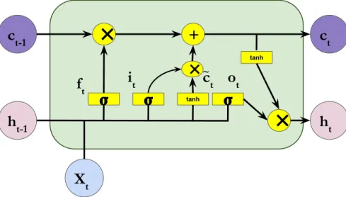
Long Short-Term Memory (LSTM) Networks were introduced byHochreiter and Schmidhuber(1997) to mitigate the issue of vanishing and exploding gradients. The LSTM is a recurrent neural network which maintains two recurrent states: a hidden state ht(similar to a vanilla RNN) and a cell state ct. The cell state is updated in

an additive manner instead of the usual multiplicative manner, which is the main source of vanishing gradients. Further, the information flow to the cell state and out of the cell state are controlled by sigmoidal gates.

Specifically, the LSTM has three di↵erent gates: forget gate ft, input gate it,

the previous hidden state ht 1.

it= sigmoid(Wxixt+ Whiht 1+ bi) (2.17)

ft= sigmoid(Wxfxt+ Whfht 1+ bf) (2.18)

ot= sigmoid(Wxoxt+ Whoht 1+ bo). (2.19)

The cell state ct is updated as follows:

˜ct= tanh(Wxcxt+ Whcht 1+ bc) (2.20)

ct= ft ct 1+ it ˜ct (2.21)

where denotes element-wise product and ˜ct is the new information to be added

to the cell state. Intuitively, ft controls how much of ct 1 should be forgotten and

it controls how much of ˜ct has to be added to the cell state.

The hidden state is computed using the current cell state as follows:

ht = ot tanh(ct). (2.22)

The LSTM maintains a cell state that is updated by addition rather than multipli-cation (see Equation 2.21) and serves as an “error carousel” that allows gradients to skip over many transition operations. The gates determine which information is skipped. Figure2.3 shows the architecture of LSTM.

X

h

c

𝛔

✕

h

c

𝛔

+

𝛔

✕

f

i

c

o

Figure 2.3 – Long Short-Term Memory (LSTM) Network.

The cell state and the hidden state in an LSTM play two di↵erent roles. While the cell state is responsible for information from the past that will be useful for future predictions, the hidden state is responsible for information from the past that

will be useful for the current prediction. Note that in a vanilla RNN, the hidden state played both these roles together. While a vanilla RNN has all the expressive power that an LSTM has, the explicit parameterization of the LSTM makes the learning problem easier. This idea of constructing explicit parameterizations to make learning easier is one of the central themes of this thesis.

The LSTM, even though introduced in 1997, is still the de-facto model that is used for most of the sequential problems. There has been few improvements to the original version of LSTM proposed byHochreiter and Schmidhuber (1997). The initial version of the LSTM did not have forget gates. The idea of adding forgetting ability to free memory from irrelevant information was introduced in

Gers et al. (2000). Gers et al. (2002) introduced the idea of peepholes connecting the gates to the cell state so the network can learn precise timing and counting of the internal states. The parameterization of an LSTM with peephole connections is given below: it = sigmoid(Wxixt+ Whiht 1+ Wcict 1+ bi) (2.23) ft = sigmoid(Wxfxt+ Whfht 1+ Wcfct 1+ bf) (2.24) ct = ftct 1+ it tanh(Wxcxt+ Whcht 1+ bc) (2.25) ot = sigmoid(Wxoxt+ Whoht 1+ Wcoct+ bo) (2.26) ht = ot tanh(ct) (2.27)

where the weight matrices from the cell to gate vectors (e.g. Wcf) are diagonal.

When we refer to LSTMs in this thesis, it is usually LSTMs with peephole connec-tions.

While the additive cell updates avoided the first source of vanishing gradients, the gradients still vanish in LSTMs due to the saturating activation functions used for gating. When the gating unit activations saturate, the gradient on the gating unit themselves vanishes. However, locking the gates to ON (or OFF) is necessary for distance gradient propagation across memory. This introduces an unfortunate trade-o↵ where either the gate mechanism receives updates or gradients are skipped across many transition operators. Due to this issue, LSTMs often end up learning only short term dependencies. However, the short term dependencies learned by LSTMs are still longer than the dependencies learned by a vanilla RNN and hence the name long short-term memory.

2.4.1

Forget gate initialization

Gers et al. (2000) proposed to initialize the bias of the forget gate to 1 which helped in modelling medium term dependencies when compared with zero initial-ization. This was also recently highlighted in the extensive exploration study by

J´ozefowicz et al.(2015). Tallec and Ollivier(2018) proposed chrono-initialization to initialize the bias of the forget gate (bf) and input gate (bi). Chrono-initialization

requires the knowledge of maximum dependency length (Tmax) and it initializes the

gates as follows:

bf ⇠ log(U[1, Tmax 1]) (2.28)

bi = bf (2.29)

This initialization method encourages the network to remember information for ap-proximately Tmax time steps. While these forget gate bias initialization techniques

encourage the model to retain information longer, the model is free to unlearn this behaviour.

2.5

Other gated architectures

A simpler gated architecture called Gated Recurrent Unit (GRU) was introduced byCho et al.(2014). Similar to LSTMs, GRUs also have gating units to control the information flow. However, unlike LSTMs which has three types of gates, GRUs has only two type of gates: an update gate zt and a reset gate rt. Both the gates

are functions of the current input xt and the previous hidden state ht 1.

zt = sigmoid(Wxzxt+ Whzht 1+ bz) (2.30)

rt = sigmoid(Wxrxt+ Whrht 1+ br) (2.31)

At any time step t, first the candidate hidden state ˜ht is computed as follows:

˜

ht = tanh(Wxhxt+ Whh(rt ht 1) + bh) (2.32)

When the reset gate is close to zero, the unit essentially forgets the previous state. This is similar to the forget gate in LSTM.

Now the hidden state ht is computed as a linear interpolation between the

previous hidden state ht 1 and the current candidate hidden state ˜ht:

ht= (1 zt) ht 1+ zt h˜t (2.33)

where the update gate zt determines how much the unit updates its content based

on the newly available content. This is very similar to the cell state update in an LSTM. However, GRU does not maintain a separate cell state. The hidden state serves the purpose of both the cell state and the hidden state in an LSTM. While the cell state helps the LSTM to remember long-term information, in GRU, it is the

duty of the update gate to learn to remember long-term information. GRUs while simpler than LSTMs, are comparable in performance to LSTMs (Chung et al.,

2014) and hence are widely used.

While GRUs reduced the number of gates in LSTM from three to two, Just Another NETwork (JANET) (van der Westhuizen and Lasenby, 2018) reduces the number of gates further to only one: the forget gate ft.

ft = sigmoid(Wxfxt+ Whfht 1+ bf) (2.34)

At any time step t, first the candidate hidden state ˜ht is computed as follows:

˜

ht= tanh(Wxhxt+ Whhht 1+ bh) (2.35)

Then the hidden state ht is computed as follows:

ht= ft ht 1+ (1 ft) h˜t (2.36)

JANET couples the input gate and the forget gate while removing the output gate. Like GRUs, JANET also does not contain an explicit cell state. van der Westhuizen and Lasenby (2018) hypothesized that it will be beneficial to allow slightly more information to accumulate than the amount of information forgotten. This can be implemented by subtracting a pre-specified value from the input control component. The modified JANET equations are given as follows:

st = Wxfxt+ Whfht 1+ bf (2.37)

˜

ht = tanh(Wxhxt+ Whhht 1+ bh) (2.38)

ht = sigmoid(st) ht 1+ (1 sigmoid(st )) h˜t (2.39)

van der Westhuizen and Lasenby(2018) showed that JANET with chrono-initialization performs better than LSTMs and LSTMs with chrono-initialization. van der West-huizen and Lasenby (2018) call this the unreasonable e↵ectiveness of the forget gate.

The fact that GRUs and JANETs, with lesser number of gates, work better than LSTMs support our hypothesis that saturating gates make learning long-term dependencies difficult. We will get back to this crucial observation in Chapter 4.

2.6

Orthogonal RNNs

Better initialization of the recurrent weight matrix has been explored in the literature of RNNs. One standard approach is orthogonal initialization where the recurrent weight matrices are initialized using orthogonal matrices. Orthogonal initialization makes sure that the spectral norm of the recurrent matrix is one during initialization and hence there is no vanishing gradient due to the recurrent weight matrix. This approach has two caveats. Firstly, the gradient would still vanish due to saturating activation functions. Secondly, this is only an initialization method. Hence, RNNs are free to move away from orthogonal weight matrices and the norm of the recurrent matrix can become less than or greater than one which would result in vanishing or exploding gradients respectively.

Le et al. (2015) addressed the first caveat using identity initialization (which results in a recurrent weight matrix with the spectral norm of one) to train RNNs with ReLU activation functions. While the authors showed good performance in a few tasks, ReLU RNNs are notoriously difficult to train due to exploding gradients. A simple way to avoid the second caveat is to add a regularization term to ensure that the recurrent weight matrix W stays close to an orthogonal matrix throughout the training. For example, one can add:

||WTW I_||2. (2.40)

Vorontsov et al. (2017) proposed a direct parameterization of W which permits a direct control over the spectral norms of the matrix. Specifically, they consider the singular value decomposition of the W matrix:

W = U SVT (2.41)

where U and V are the orthogonal basis matrices and S is a diagonal spectral matrix that has the singular values of W as the diagonal entries. The basis matrices U and V are kept orthogonal by doing geodesic gradient descent along the set of weights that satisfy U UT _{= I and VV}T _{= I respectively. If we fix the S matrix to}

be an identity matrix, we can ensure the orthogonality of W matrix throughout the training. However, Vorontsov et al.(2017) proposes to parameterize the S matrix in such a way that the singular values can deviate from 1 by a margin of m. This is achieved with the following parameterization:

si = 2m( (pi) 0.5) + 1, si 2 {diag(S)}, m 2 [0, 1] (2.42)

This parameterization guarantees that the singular values are restricted to the range [1 m, 1 + m] while the underlying parameters pi are updated by using the

maintaining the hard orthogonal constraint can be overall detrimental. Authors hypothesise that orthogonal RNNs cannot forget information and this might be problematic in tasks that require only short-term dependencies. On the other hand, allowing the singular values to deviate from 1 by a small margin consistently improved the performance. Deviating by a large margin can lead to vanishing and exploding gradients.

2.7

Unitary RNNs

Another line of work starting from (Arjovsky et al., 2016) explored the idea of using unitary matrix parameterization for recurrent weight matrix. Unitary matrices generalize orthogonal matrices to the complex domain. The spectral norm of the unitary matrices is also one. Arjovsky et al. (2016) proposed a simple parameterization of unitary matrices based on the observation that the product of unitary matrices is a unitary matrix. Their parameterization ensured that one can do gradient descent on the parameters without deviating from the unitary recurrent weight matrix.

Wisdom et al. (2016) observed that the parameterization of Arjovsky et al.

(2016) does not span the entire space of unitary matrices and proposed an alternate parameterization that has full capacity. To stay in the manifold of unitary matrices,

Wisdom et al. (2016) has to re-project the recurrent weight matrix to the unitary space after every gradient update. Jing et al. (2017b) avoids the re-projection cost by using an efficient unitary RNN parameterization with tunable representation capacity which does not require any re-projection step. This model is called the Efficient Unitary Neural Network (EUNN).

One issue with orthogonal and unitary matrices is that they do not filter out information, preserving gradient norm but making forgetting impossible. Gated Orthogonal Recurrent Units (GORUs) (Jing et al., 2017a) addressed this issue by combining Unitary RNNs with a forget gate to learn to filter the information. It is worth noting that Unitary RNNs are, in general, slow to train due to the inherent sequential computations in the parameterizations. Restricting the recurrent weight matrices to be orthogonal or unitary also restricts the representation capacity of an RNN.

2.8

Statistical Recurrent Units

Statisti-cal Recurrent Units (SRUs). SRUs model sequential information by using recurrent statistics which are generated at multiple time scales. Specifically, SRUs maintain exponential moving averages m(↵) _{defined as follows:}

m(↵)_t = ↵m(↵)_{t 1}+ (1 ↵) ˆmt (2.43)

where ↵ 2 [0, 1) defines the scale of the moving average and ˆmt is the recurrent

statistics at time t computed as follows:

rt= f (Wrmt 1+ br) (2.44)

ˆ

mt= f (Wmrt+ Wxxt+ bm) (2.45)

where f is a ReLU activation function. As we can see, the recurrent statistics at time t is conditioned on the current input and on the recurrent statistics at the previous time step. Oliva et al.(2017) proposed to consider m di↵erent values for ↵ (where m is a hyper-parameter) to maintain the recurrent statistics at multiple time scales. At any time-step t, let mt denote the concatenation of all such recurrent

statistics.

mt= [m↵t1; m↵t2; ...; m↵tm] (2.46)

Now the hidden state of the SRU is computed as follows:

ht = f (Whmt+ bh) (2.47)

SRUs handle the vanishing gradients by having an ungated architecture with ReLU activation function and simple recurrent statistics. However, it is worth noting that the recurrent statistics are computed by using exponential moving averages which will shrink the gradients.

2.9

Memory Augmented Neural Networks

Memory augmented neural networks (MANNs) (Graves et al., 2014; Weston et al.,2015) are neural network architectures that have access to an external mem-ory (usually a matrix) which it can read from or write to. The external memmem-ory matrix can be considered as a generalization of the cell state vector in an LSTM. In this section, we will introduce two memory-augmented architectures: Neural Tur-ing Machines (Graves et al.,2014) and Dynamic Neural Turing Machines (Gulcehre et al., 2016).

2.9.1

Neural Turing Machines

Memory

Memory in Neural Turing Machine (NTM) is a matrix Mt 2 Rk⇥q where k is

the number of memory cells and q is the dimensionality of each memory cell. The controller neural network can use this memory matrix as a scratch pad to write to and read from.

Model Operation

The controller in an NTM can either be a feed-forward network or an RNN. The controller has multiple read heads, write heads, and erase heads to access the memory. For this discussion, we will assume that the NTM has only one head per operation. However, this description can be easily extended to the multi-head setting.

At each time step t, the controller receives an input xt. Then it generates the

read weight wr

t 2 Rk⇥1. The read weights are used to generate the content vector

rt as a weighted combination of all the cells in the memory:

rt= MTtwrt 2 Rq⇥1 (2.48)

This content vector is used to condition the hidden state of the controller. If the controller is a feed-forward network, then the hidden state of the controller is defined as follows:

ht= f (xt, rt) (2.49)

where f is any non-linear function. If the controller is an RNN, then the hidden state of the controller is computed as:

ht = g(xt, ht 1, rt) (2.50)

where g can be a vanilla RNN or a GRU network or an LSTM network.

The controller also updates the memory with a projection of the current hidden state. Specifically, it computes the content to write as follows:

at= f (ht, xt) (2.51)

It also generate write weights ww

t 2 Rk⇥1 in similar way as read weights and erase

as follows:

Mt[i] = Mt 1[i](1 wwt[i]et) + wwt[i]at (2.52)

Intuitively, the writer erases some content from every cell in the memory and adds a weighted version of the new content to every cell in the memory.

Thus in every time step, the controller computes the current hidden state as a function of the content vector generated from the memory. Also, at every time step, the controller writes the current hidden state to the memory. Thus, even if the controller is a feed-forward network, the architecture is recurrent due to the conditioning on the memory.

Addressing Mechanism

Now we will describe how the read head generates the read weights to address the memory cells. The write heads generate their write weights in a similar manner. In NTMs, memory addressing is a combination of content-based addressing and location-based addressing.

The read head first generates a key for memory access:

kt= f (xt, ht 1)2 Rq⇥1 (2.53)

The key is compared with each cell in the memory Mt by using some similarity

measure S to generate the content-based weights as follows: wc_t = Pexp( tS[kt, Mt[i]])

jexp( tS[kt, Mt[j]])

(2.54) where tis a positive key strength vector that can amplify or attenuate the precision

of the focus.

Next, the read head generates a scalar interpolation gate gt 2 (0, 1) which is

used to interpolate between the content-based addressing and the previous address wr

t 1. The interpolated weight w g

t is defined as follows:

wgt = gtwtc+ (1 gt)wt 1r (2.55)

If the gating weight is one, then the previous weight is ignored and only the content-based weight is considered. If the gating weight is zero, then the content-content-based weight is ignored and only the previous weight is considered. This interpolated weight is passed as input to the location-based addressing.

After interpolation, the read head generates a shifting weight st which defines

a normalized distribution over the allowed integer shifts. If the memory locations are indexed from 0 to k-1, then the rotation applied to wgt by st can be expressed

as a circular convolution: ˜ wt[i] = k 1 X j=0 wg_t[j]st[i j] (2.56)

where the indices are computed modulo N. The convolution operation may cause leakage of weight over time if the shift weight is not sharp. This is addressed by generating a scalar t 1 which is used to sharpen ˜wtto produce the final weights:

wr_t[i] = w˜t[i]

t

P

jw˜t[j] t

(2.57)

This addressing mechanism can learn to operate in three modes: pure content-based addressing, pure location-content-based addressing, content-content-based addressing follow-ing by location-based shiftfollow-ing. As we can see, the entire addressfollow-ing mechanism is continuous and hence the architecture is fully di↵erentiable. Graves et al. (2014) showed that NTMs can easily solve several algorithmic tasks which are very dif-ficult for LSTMs. NTMs inspired a series of memory augmented architectures: Dynamic NTMs (Gulcehre et al., 2016), Sparse Access Memory (Rae et al., 2016), and Di↵erentiable Neural Computer (Graves et al., 2016). We will describe only the Dynamic NTM architecture, which is more relevant to this thesis.

2.9.2

Dynamic Neural Turing Machines

Memory

The memory matrix Mt2 Rk⇥q in the Dynamic NTM (D-NTM) is partitioned

into two parts: the address part At2 Rk⇥da and the content part Ct2 Rk⇥dc such

that da+ dc = q.

Mt= [At; Ct] (2.58)

The address part is considered to be a model parameter and is learned during training. During inference, the address part is frozen and is not updated. On the other hand, the content part is updated during both training and inference. Also, the content part is reset to zero for every example, C0 = 0. The learnable address

part allows the model to learn more sophisticated location-based strategies when compared to the location-based addressing used in NTMs.

Model Operation

Like NTMs, the controller in D-NTMs can either be a feed-forward network or an RNN. At each time step t, the controller receives an input xt. Then it generates

the read weights wr

t 2 Rk⇥1. The read weights are used to generate the content

vector rt as a weighted combination of all the cells in the memory:

rt= MTtwrt 2 Rq⇥1. (2.59)

This content vector is used to condition the hidden state of the controller. If the controller is a feed-forward network, then the hidden state of the controller is defined as follows:

ht= f (xt, rt), (2.60)

where f is any non-linear function. If the controller is an RNN, then the hidden state of the controller is computed as:

ht= g(xt, ht 1, rt), (2.61)

where g can be a vanilla RNN or a GRU network or an LSTM network.

Similar to the NTM, the controller in D-NTM also updates the memory with a projection of the current hidden state. Specifically, it computes the content vector ct2 Rdc⇥1 to write as follows:

ct= ReLU(Wmht+ ↵tWxxt), (2.62)

where ↵t is a scalar gate controlling the input. It is defined as follows:

↵t= f (ht, xt). (2.63)

The controller also generates write weights ww

t 2 Rk⇥1 in similar way as read

weights and erase vector et 2 Rdc⇥1 whose elements are in the range (0,1). It

updates the content of each cell Ct[i] as follows:

Ct[i] = Ct 1[i](1 wtw[i]et) + wwt [i]ct. (2.64)

Intuitively, the writer erases some content from every cell in the memory and adds a weighted version of the new content to every cell in the memory. Unlike NTMs, D-NTMs have a designated No Operation (NOP) cell in the memory. Reading from or writing to this NOP cell is ignored. This is used to add the flexibility of not accessing the memory at any time step.

Addressing Mechanism

We describe the addressing mechanism for the read head here. But the same description holds for the write heads as well.

The read head first generates a key for the memory access:

kt= f (xt, ht 1)2 Rq⇥1. (2.65)

The key is compared with each cell in the memory Mt by using some similarity

measure S to generate the logits for the address weights as follows:

zt[i] = tS[kt, Mt[i]], (2.66)

where t is a positive key strength vector that can amplify or attenuate the

pre-cision of the focus. Up to this point, the addressing mechanism looks like the content-based addressing in the NTM. But note that the memory also has a loca-tion part and hence this adressing mechanism is a mix of content-based addressing and location-based addressing.

While writing, sometimes it is e↵ective to put more emphasis on the least re-cently used (LRU) memory locations so that the information is not concentrated in only few memory cells. To implement this e↵ect, D-NTM computes the moving average of the logits as follows:

vt= 0.1vt 1+ 0.9zt. (2.67)

This accumulated vt is rescaled by a scalar gate t 2 (0, 1) and subtracted from

the current logits before applying the softmax operator. The final weight is given as follows:

wr_t = softmax(zt tvt 1). (2.68)

By setting t to 0, the model can choose to use pure content-based addressing.

This is known as dynamic LRU addressing since the model can dynamically decide whether to use LRU addressing or not.

D-NTM uses single head with multi-step addressing similar toSukhbaatar et al.

(2015) instead of multiple heads used by the NTM.

Discrete Addressing wr

t in Equation 2.68 is a continuous vector and if used as such, the entire

ar-chitecture is di↵erentiable. The D-NTM with continuous wr