Detection of nonlinearity in a dynamic system using deformation modes obtained from the Wavelet Transfrom of measured responses

DETECTION OF NONLINEARITY IN A DYNAMIC SYSTEM

USING DEFORMATION MODES OBTAINED FROM

THE WAVELET TRANSFORM OF MEASURED RESPONSES

NGUYEN V. H., PEETERS M., GOLINVAL J.-C. University of Liege,

Aerospace and Mechanical Engineering Department, Structural Dynamics Research Group Chemin des Chevreuils 1, B52, B-4000 Liege, Belgium

Email : VH.Nguyen@doct.ulg.ac.be, M.Peeters@ulg.ac.be, JC.Golinval@.ulg.ac.be

SUMMARY: An efficient approach to Structural Health Monitoring of dynamical systems based on the Wavelet Transform (WT) and the concept of subspace angle is presented. The objective is to propose a detection method that is sensitive to the onset of nonlinear behaviour in a dynamic system. For this purpose, instantaneous frequencies are identified first from output-only vibration signals using the Wavelet Transform. Time varying deformation shapes are then extracted by analyzing the whole measurement data set on the structure. From this information, different dynamic states of the structure may be detected by inspecting time variations of ‘modal’ features. The experimental structure considered here as application example is a clamped beam with a geometric nonlinearity. Detection of nonlinearity is carried out by means of the concept of subspace angles between instantaneous deformation modes extracted from measurement data using the continuous Wavelet Transform. The method consists in controlling the angular coherence between active subspaces of the current and reference states respectively. The proposed technique, which shows a good sensitivity to small changes in the dynamic behaviour of the structure, may also be used for damage detection.

KEYWORDS: identification, nonlinearity, detection, subspace angle. 1. INTRODUCTION

Detection of changes in the dynamic state of structures is an important issue in the field of Structural Health Monitoring (SHM). It may be caused by the occurrence of damage but also by the onset of a nonlinear behaviour. Detection methods based on output-only vibration measurements attempt to extract features which are sensitive to changes in the current dynamic state of the monitored structure.

Detection methods that use mathematical models include parametric and non-parametric techniques. Parametric methods require the construction of a structural model and are based on model updating techniques [1-3]. A precise model is of primary importance in this case; it offers the advantage to allow damage location and possibly remaining lifetime calculation but it generally needs a lot of modelling and computation time. Non-parametric methods do not require a structural model. They may be based on the direct use of modal parameters (natural frequencies and mode shapes), or stiffness and flexibility matrices. For example, some techniques are based on principal component analysis (PCA) of vibration measurements [4] or on a combination of independent component analysis (ICA) with neural networks [5]. However, most of the methods are based on the assumption of stationarity of the signals and lead to the identification of a unique set of ‘modal’ features. Time-frequency decompositions are helpful to capture transient dynamic features that appear during operation. One of them is the Hilbert-Huang transform (HHT) [6] that has been developed in the last decade to handle both identification and detection problem [7-8]. One of the main drawbacks of the HHT method relies in its empirical formulation. Conversely the theoretical basis of the Wavelet Transform (WT) makes it more appropriate for non-stationary data analysis. Gurley et al [9] used both the continuous and discrete WT for identification and characterization of transient random processes. Using Morlet wavelet, Kijewski et al. [10] deal with system identification in civil engineering and Staszewski [11] with identification of systems with cubic stiffness nonlinearity. Argoul, Le and Erlicher [12-14] use the continuous Cauchy wavelet transform as a tool for modal identification in linear and nonlinear systems. In [12], four instantaneous indicators are proposed to facilitate the characterization of the nonlinear behaviour of a structure.

The aim of this paper is to propose an alternative method to detect nonlinearity using the Wavelet Transform and the concept of subspace angles. Morlet wavelet is considered here as the mother wavelet to extract instantaneous frequencies and amplitudes from time measurements at different locations on the structure. Deformation modes associated to instantaneous frequencies may then be extracted from the whole data set and assembled to build

instantaneous observation matrices. Singular value decomposition of these matrices allows to determine the dimensionality of the system. Next, the retained deformation shapes are compared with reference mode-shapes using the concept of subspace angle. The objective is to provide an index able to detect the onset of the nonlinear behaviour of the structure. The proposed technique is illustrated on the example of a clamped beam which exhibits a geometric nonlinearity at one end. It shows a good sensitivity to small changes in the dynamic behaviour of the structure and thus may also be used for damage detection.

2. WAVELET TRANSFORM (WT)

The wavelet transform consists in decomposing the signal f t( )∈L2( )ℜ into a series of basis functions expressed by dilated and translated versions of the mother wavelet through the convolution of the signal and the scaled mother wavelet according to:

( )t ψ 1 ( , ) ( ) t u Wf u s f t dt s s ψ +∞ −∞ − ⎛ ⎞ = _{⎜ ⎟} ⎝ ⎠

∫

The function ψ with zero mean must be admissible to permit the analysis of the signal and its reconstruction without loss of information. The wavelet coefficients, , designate the similitude between the dilated and translated mother wavelet and the signal at the time t and at the scale (frequency) s. Thanks to its ability to consider time and frequency resolutions at the same time, the WT is particularly well adapted to detect discontinuity or sharp signal transitions.

( , ) Wf u s

To separate amplitude and phase information of signals, one uses analytic complex wavelets, i.e. its Fourier transform ψ ωˆ ( )=0forω< . Many analytic wavelets are studied in the literature. The choice of mother wavelet 0 depends on several analysis properties. The Morlet wavelet which is considered in this work is defined by:

0 ( ) ( ) j t M t g t eω ψ = with 2 2 4 2 ₂ ( ) 1/ . t g t = πσ e− σ (2)

where ω is the centre frequency of ₀ ψ and the parameter ˆ σ arranges time and frequency resolutions. If , the wavelet is considered as approximately analytical with zero mean and admissible. The FT of reaches the maximum at

2 2 0 1

σ ω >> ( )

M t

ψ sω ω= ₀ and it leads to a relation between instantaneous frequency and scale:

0/ s

ω ω= .

2.1. Wavelet ridges

If a(u) and φ( )u are respectively instantaneous amplitude and phase, the WT is also given by:

( )

_{

₍

₎

₍

)

}

( )

'( )u

φ Wf u s( , ) φ'( )u

,

u s

ψ and φ'( )u ≥ Δω/s, that Δ is bandwidth of ω gˆ.

Different methods exist to define and to extract ridges [11, 12, 15]. The scalogram gives a time-frequency representation of the energy contained in the signalf t( ). The frequencies that correspond to the maximum of constitute the ridge. Here, the ridge algorithm computes instantaneous frequencies from local maxima of the scalogram, corresponding to dominant frequency components in the signal at each time instant. If

( , ) Wf u s

(

W uη

)

Φ is the complex phase of , at ridge points, the instantaneous frequency and the analytic amplitude a(u) are given respectively by:

( , ) Wf u s φ'( )u

( )

( )

3. DETECTION BASED ON THE CONCEPT OF SUBSPACE ANGLE

For a given excitation, the WT allows to identify the instantaneous frequencies (or ridges) at a set of different measurement coordinates on the structure. Accordingly, it provides the amplitude ratios between coordinates in each instantaneous deformation mode associated to an identified ridge line. Using these ratios, one can assess time-varying deformation (‘mode’) shapes of the system. The modes with the strongest energies may be regarded as active modes and used to construct active subspaces at different time instants (or states of the system). A change in the dynamic behaviour modifies consequently the state of the system, i.e. the instantaneous frequencies and deformation shapes. This change may be estimated using the concept of subspace angle introduced by G.H. Golub and C.F. Van Loan [16]. This concept was used in [4] as a tool to quantify existing spatial coherence between two data sets resulting from observation of a vibration system. Given two subspaces (each with linear independent columns) S∈ ℜn p× and D∈ ℜn q× (p>q), the procedure is as follows. Carry out the QR factorizations: S = QSRS (QS n p ×

ℜ

∈

ℜ

∈

the orthonormal bases for S and D respectively. The angles

θ

Q Q = UT_{S D SD}

Σ

(

( )

)

The onset of nonlinearity in a structure may be detected by monitoring the angular coherence between subspaces estimated from the reference observation set and from the observation set of a current state respectively. A state is considered as a reference state if the system operates in normal condition (nonlinearity is not activated or damage does not exist).

4. WT APPLICATION TO DETECT NONLINEARITY

The example consists in identifying the modal features and in detecting the level of nonlinearity in a cubic stiffness system by means of the WT. The analysis is conducted both numerically and experimentally. The studied structure is a beam clamped at one end and exhibiting a cubic stiffness at the other end (figure 1). The cubic stiffness is realised by means of a very thin beam. For weak excitation, the system behaviour may be considered as linear. When the excitation level increases, the thin beam exhibits large displacements and a nonlinear geometric effect is activated resulting in a stiffening effect at the end of the main beam.The structure was used as a benchmark for nonlinear system identification during the European action COST F3 [12, 19].

a)

b)

Figure 1 - The beam with a nonlinear stiffness (a) and its finite element model (b)

4.1. Numerical analysis

The main beam is modelled with seven beam finite elements (figure 1b). The thin beam is represented by two equivalent grounded springs: one in translation (kl + knl) and one in rotation (kr). The nonlinear stiffening effect

of the thin beam is modelled by a nonlinear function in displacement of the form:f_nl( )x =A xαsign( )x , where A is a nonlinear coefficient, _{A= ×6 10}9_{N m/} 3

and α is a nonlinear exponent,α= . These parameters were 3 determined experimentally in reference [19].

Nonlinear normal modes

The nonlinear normal modes (NNMs) of this structure were calculated in reference [18]. These modal features depend on the total energy in the system as illustrated in figure 2 by the frequency-energy plot (FEP) of the first and the second NNMs.

a) First NNM b) Second NNM Figure 2 - Frequency-energy plot of the first (a) and second (b) NNMs

The first and second NNM motions are plotted in figure 3 at low and high energy level respectively. The low energy level (actually the linear normal modes) corresponds to f1 = 32.60 Hz and f2 = 144.79 Hz while the high

energy level (the nonlinear case) corresponds to f1 = 38.46 Hz and f2 = 147.67 Hz.

Figure 3 - Analytical deformation shapes of the 1st, 2nd modes respectively

Impact excitation

For the purpose of this study, the beam is supposed to be submitted to an impact force at its right end. The free response of the structure is measured in the vertical direction at the seven coordinates indicated in figure 1b and the WT is applied to the measured data. Starting at a ‘low’ excitation level (impact of 70N), the behaviour of the beam appears as linear (the largest displacement is lower than 0.15 mm). The WT of the displacement at coordinate n°7 is given in figure 4 in terms of instantaneous frequencies and amplitudes. Two frequency lines (called ‘ridges’) are observed respectively at 32.6 Hz and 144.7 Hz, which is in agreement with the frequencies occurring at low energy in the FEP (figure 2). Higher frequencies of small amplitudes could also be detected [19] but they are not considered here.

Figure 4 - Instantaneous frequencies and amplitudes at low energy (linear case)

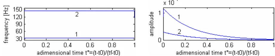
Let us consider next a high level of excitation (impact of 1500N) corresponding to a maximum displacement at the right end of about 2.4 mm. Figure 5 presents the corresponding WT results. It clearly shows a drop-off of the frequencies down to the linear system values as the nonlinear effect vanishes progressively and the amplitude goes down. Figure 5 also reveals the presence of a 3 order super harmonic of the first frequency (curve n° 3).

Figure 5 - Instantaneous frequencies and amplitudes at high energy (nonlinear case)

Identification of deformation shapes and detection of nonlinear behaviour

Figure 6 presents the first two modes of the beam identified with the ‘low’ impact excitation when the dynamic behaviour of the structure may be considered as linear.

Figure 6 - Mode 1 and 2 in the linear case

Figure 7 gives the deformation shapes at higher excitation levels. When the displacement at the right end starts to be significant, both the first two deformation shapes associated to ridges n° 1 and n° 2 become influenced by the magnitude of the nonlinearity of the structure (the reference shape corresponds to the linear normal modes shown in figure 6). For high excitation levels, a super harmonic of the first frequency appears as illustrated by the ridge line n° 3 in figure 5. It is interesting to note that one can find an intermediate deformation shape from this ridge line; the last plot of figure 7 gives the corresponding deformation shapes for different amplitudes of the displacement at the right end of the beam.

Figure 7 - Deformation shapes associated to the 1st, the 2nd and the super harmonic modes

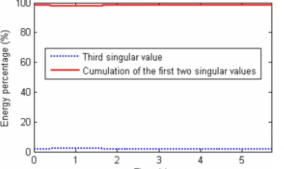
The instantaneous deformation shapes M1, M2 and M3 corresponding to the three ridges allow defining an

instantaneous deformation matrix A = [M1 M2 M3]. Performing the singular-value decomposition (SVD) of

matrix A, it can be shown that the third (super harmonic) deformation mode (M3) is actually a linear

combination of the two other modes. Figure 8 shows the instantaneous singular values of the decomposition in terms of energy percentage. It reveals that the third singular value is negligible compared to the two others.

Figure 8 - Instantaneous singular values of the deformation mode matrix

a) Displacement amplitude ≈ 0.6 mm b) Displacement amplitude ≈ 1.25 mm c) Displacement amplitude ≈ 2.3 mm Figure 9 - MAC between WT and SSI modes

The comparisons may be equally carried out by means of the MAC (Modal Assurance Criterion). In figure 9, deformation modes obtained through the WT are compared with the linear normal modes identified by the SSI

method (Stochastic Subspace Identification) for different values of the displacement at the end of the beam. When the displacement is low (figure 9a), the MAC indicates a perfect correlation. At this level of excitation, the deformation shapes are identical to the linear normal modes. On the other hand, when the displacement amplitude is high (figure 9c), the nonlinearity is well excited which results in a frequency increase and a slight loss of correlation with the linear normal modes (identified by SSI). Figure 9 shows however that the MAC is not a deciding criterion for the detection of nonlinearity.

Detection based on the concept of subspace angle

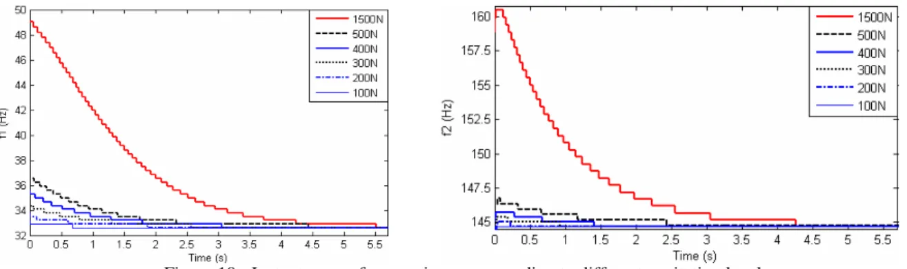
For the purpose of detection of nonlinearity, the structure is now supposed to be excited at increasing level of impact force (amplitudes ranging from 100 N to 1500 N). The corresponding instantaneous frequencies obtained through the WT of the response signals at coordinate n°7 are shown in figure 10.

Figure 10 - Instantaneous frequencies corresponding to different excitation levels

As explained in section 3, the instantaneous deformation shapes associated to these two frequencies may be considered as instantaneous active modes to define a subspace which characterises the dynamic state of the structure. The comparison of subspace angles between the reference state (defined by the linear normal modes) and current states at different excitation levels reveals the range of activation of the nonlinearity as illustrated in figure 11. Larger is the excitation level, more significant is the angle. As responses are damped, the angles reach their largest values at the beginning and then decrease gradually to converge to zero as the dynamic behaviour of the beam becomes linear.

a) Based on the 1st deformation mode b) Based on the 2nd deformation mode c) Based on the both 2 deformation modes

Figure 11 - Time evolution of subspace angles for different excitation levels

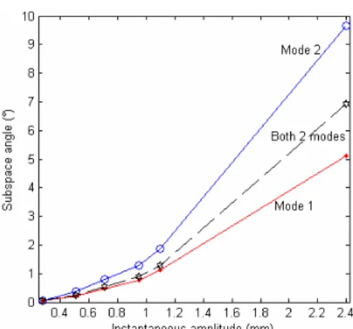
As the activation of the nonlinearity depends on the amplitude level of the displacement, the display of subspace angles according to the evolution of the instantaneous displacement amplitude measured at the end of the beam is informative. Figure 12 shows the evolution of subspace angles in function of the displacement amplitude measured at the end of the beam at time t = 0.1 s. It can be observed that the subspace angle criterion for the 2nd mode is more sensitive to the nonlinearity in comparison to the 1st mode (which is confirmed by the MAC in figure 9). In terms of frequency changes however, the 1st mode appears as more affected than the 2nd mode (figure 10).

In summary, the onset of nonlinearity may be detected by observing the evolution of instantaneous frequencies as illustrated in figure 10 but a high frequency resolution is needed to distinguish between close levels of excitation (e.g. impacts of 100 N to 500 N). In this respect, subspace angle curves look more promising as they look less affected by the frequency resolution. Another advantage is that the concept of subspace angle allows to handle several modes simultaneously in a unique detection index.

Figure 12 - Relation angle–displacement amplitude at the end of the beam at t = 0.1s 4.2. Experimental results

Experimental results were collected using 7 accelerometers located at the coordinates given in figure 1.

An impact of very low amplitude was first applied at the end of the beam to obtain the reference state. The first two natural frequencies are observed at 31.3 Hz and 143.5 Hz respectively as shown in figure 13 which gives the WT of the response measured at the end of the beam (coordinate n° 7). These values are slightly lower than the frequencies predicted by the numerical model, which is mainly due to the influence of the mass of the sensors.

Figure 13- Instantaneous frequencies and amplitudes corresponding to an impact of low amplitude

An impact of higher amplitude was then applied to activate the nonlinearity. The results are shown in figure 14. It is observed that three instantaneous frequencies (ridges) are detected and that they are decreasing in time.

Figure 14 - Instantaneous frequencies and amplitudes when the nonlinearity is activated

The deformation modes corresponding to those three frequencies are presented in figure 15 at different instants (corresponding to different levels of displacement at the end of the beam).

a) From the first frequency ridge b) From the second frequency ridge c) From the third frequency ridge Figure 15 - Deformation modes corresponding to different displacement amplitudes

The singular-value decomposition (SVD) of matrix A = [M1 M2 M3] confirms that the third deformation mode

Figure 16 - Instantaneous singular values of the deformation mode matrix

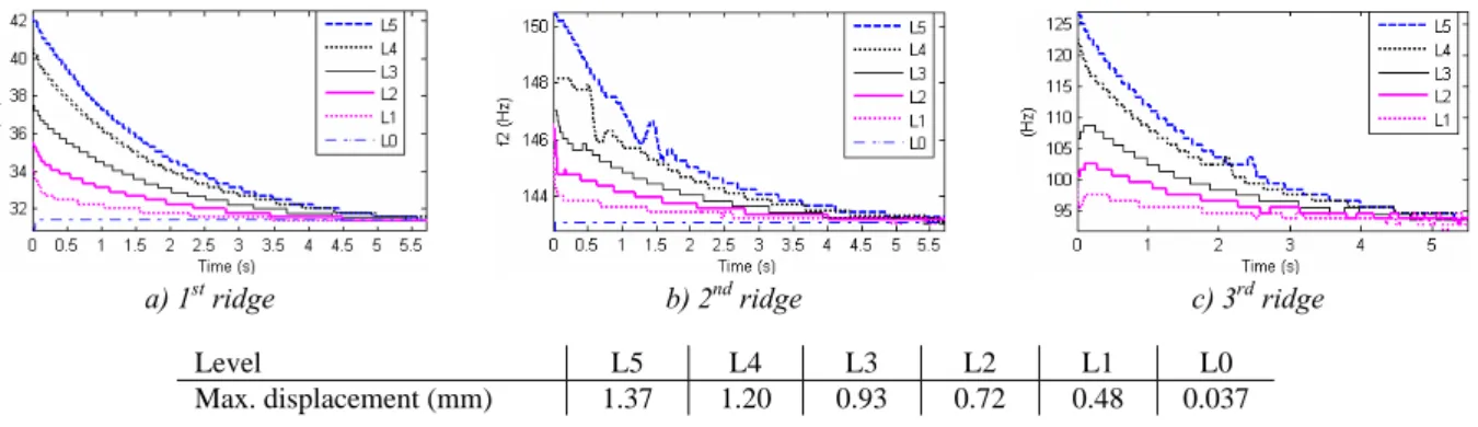
In the following, the experiments were performed for 6 levels of excitation (L0-L5). The results of the WT in terms of instantaneous frequencies are given in figure 17.

a) 1st _{ridge b) 2}nd _{ridge c) 3}rd _ridge

Level L5 L4 L3 L2 L1 L0

Max. displacement (mm) 1.37 1.20 0.93 0.72 0.48 0.037

Figure 17 - Instantaneous frequencies

Figure 18 gives the time evolution of subspace angles for the 6 levels of excitation. The angles are calculated respectively on the basis one single deformation mode (M1 or M2) in figure 18 a)-b) and on the basis of the two

independent ‘modes’ obtained through the SVD of the deformation mode matrix in figure 18 c).

a) b) c)

Figure 18 - Time evolution of subspace angles for different excitation levels on the basis of ‘mode’ 1 (a), ‘mode’ 2 (b) and SVD modes (c)

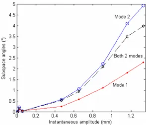
Detection results are also given in terms of displacement amplitude in figure 19. It can be seen how the magnitude of the nonlinearity depends on the displacement level. ‘Mode’ 2 looks more sensible to the nonlinearity than ‘mode 1’.

Figure 19 - Relation angles–displacement amplitudes at the end of beam, based on each ‘mode’, t = 0.125s

5. CONCLUSION

The Wavelet Transform is known for its ability to analyze non-stationary signals and to detect nonlinear behaviour in a structure. As reported in [12], it can be used to identify instantaneous frequencies.

In this paper, detection of nonlinearity in a dynamic system submitted to impact excitation was performed using the concept of subspace angles between instantaneous deformation modes. These deformation modes are associated to instantaneous frequencies obtained from the wavelet transform of vibration signals measured at different coordinates of the system. Instantaneous bases of independent modes may be generated using the singular value decomposition of deformation mode matrices, which determines the dimensionality of the system. The procedure was illustrated both numerically and experimentally on the example of a nonlinear cantilever beam. The concept of subspace angles allows to define a global detection index which is sensitive to small dynamic changes and which looks robust to frequency resolution.

ACKNOWLEDGEMENTS

The first author would like to thank Prof. P. Argoul and Dr. B. Godard for their help in the use of the WT. 6. REFERENCES

[1] Friswell M.I., Mottershead J.E., Ahmadian H., “Finite-element model updating using experimental test data: parametrization and regularization”, Transactions of the Royal Society of London, Series A, Special Issue on Experimental Modal Analysis, 359(1778), January 2001, pp.169-186.

[2] Titurus B., Friswell M.I., Starek L., “Damage detection using generic elements. Part I. Model updating”, Computers and Structures 81, 2003, pp.2273-2286.

[3] Titurus B., Friswell M.I., Starek L., “Damage detection using generic elements. Part II. Damage detection”, Computers

and Structures 81, 2003, pp.2287-2299.

[4] De Boe P., Golinval J.C., “Principal component analysis of a piezosensor array for damage localization”, Structural Health Monitoring, 2003, pp.137-144.

[5] Zang C., Friswell M.I., Imregun M., “Structural damage detection using independent component analysis”, Structural Health Monitoring 3, 2004, pp.69-83.

[6] Huang N. et al. “The empirical mode decomposition and Hilbert spectrum for nonlinear and nonstationary time series analysis”. Pro. R. Soc. London (1998), Ser. A, 454, 903-995.

[7] Wu Z., Huang N.. “Ensemble empirical mode decomposition: a noise-assisted data analysis method”. Advances in Adaptive Data Analysis, Vol. 1, No.1 (2009), pp. 1-41.

[8] Yang J.N., Lei Y., Lin S., Huang N., “Hilbert – Huang based approach for structural damage detection”, Journal of Engineering Mechanics, No. 1, January 2004.

[9] Gurley K., Kareem A., “Applications of wavelet transforms in Earthquake, Wind and Ocean Engineering”, Engineering

Structures 21, 1999, pp.149-167.

[10] Kijewski T., Kareem A., “Wavelet transforms for system identification in civil engineering”, Computer-aided civil and Infrastructure Engineering 18, 2003, pp.339-355.

[11] Staszewski W. J., “Identification of non-linear systems using multi-scale ridges and skeletons of the Wavelet transform”. Journal of Sound and Vibration (1998) 214 (4), pp.639-658.

[12] Argoul P. and Le T.-P., “Instantaneous indicators of structural behaviour based on the continuous Cauchy wavelet analysis”, Mechanical Systems and Signal Processing 17(1), 2003, pp.243-250.

[13] Le T.-P., Argoul P., “Continuous wavelet transform for modal identification using free decay response”, Journal of Sound and Vibration 277, Issues 1-2, 6 October 2004, pp.73-100.

[14] Erlicher S., Argoul P., “Modal identification of linear non-proportionally damped systems by wavelet transform”, Mechanical Systems and Signal Processing 21, April 2007, pp.1386-1421.

[15] Mallat, “A wavelet tour of signal processing”. Academic press, 1999.

[16] Golub G.H., Van Loan C.F., “Matrix computations” (3rd ed.), Baltimore, TheJohns Hopkins University Press, 1996.

[17] Kerschen G., Peeters M., Golinval J.C., Vakakis A., “Nonlinear Normal Modes, Part I: An Attempt To Demystify Them”. Proceedings of the International Modal Analysis Conference, 2008.

[18] Peeters M., Viguié R., Sérandour G., Kerschen G., Golinval J.C., “Nonlinear Normal Modes, Part II: Practical Computation using Numerical Continuation Techniques”. Proceedings of the International Modal Analysis Conference, 2008.

[19] Lenaerts V., Kerschen G., Golinval J.C., Proper Orthogonal Decomposition for Model Updating of Non-linear Mechanical Systems, Journal of Mechanical Systems and Signal Processing, 15(1), pp.31-43, 2001.