Image Characterization from Statistical Reduction of Local Patterns

HAL Id: hal-01130930

https://hal.archives-ouvertes.fr/hal-01130930

Submitted on 12 Mar 2015

HAL is a multi-disciplinary open access

archive for the deposit and dissemination of

sci-entific research documents, whether they are

pub-lished or not. The documents may come from

teaching and research institutions in France or

abroad, or from public or private research centers.

L’archive ouverte pluridisciplinaire HAL, est

destinée au dépôt et à la diffusion de documents

scientifiques de niveau recherche, publiés ou non,

émanant des établissements d’enseignement et de

recherche français ou étrangers, des laboratoires

publics ou privés.

Image Characterization from Statistical Reduction of

Local Patterns

Philippe Guermeur, Antoine Manzanera

To cite this version:

Philippe Guermeur, Antoine Manzanera. Image Characterization from Statistical Reduction of Local

Patterns. Iberoamerican Congress on Pattern Recognition, Nov 2009, Guadalajara, Mexico.

�hal-01130930�

S t a t i s t i c a l R e d u c t i o n o f L o c a l P a t t e r n s .

Philippe Guermeur and Antoine Manzanera

ENSTA, 32 Bd Victor, 75015 Paris CEDEX 15, France. Tel: 33 (1) 45 52 54 87. E-mail: philippe.guermeur@ensta.fr.

WWW: http://www.ensta.fr/~guermeur

Abstract. This paper tackles the image characterization problem from a sta-tistical analysis of local patterns in one or several images. The induced image characteristics are not defined a priori, but depends on the content of the im-ages to process. These characteristics are also simple image descriptors and thus considering an histogram of these elementary descriptors enables to ap-ply "bags of words" techniques. Relevance of the approach is assessed when dealing with the image recognition problem in a robot application framework.

1

Introduction

Local image description techniques usually relate to interest point detection methods. Many image processing methods define the notion of interest point from using a theo-retical model of gray level variations on a local image neighbourhood [1], [2], [3]. More recent approaches combine interest points to image descriptors. A typical approach is the SIFT method which computes histograms from gradient orientations near interest points locations. [4] gives an overview of these various approaches which have often been used in "bags of words" methods for image indexing applications or robot navigation tasks such as Simultaneous Localization and Mapping of the Environ-ment (SLAM). All of these techniques define the notion of interest point from design-ing an a priori model of what is a corner or some other interestdesign-ing geometric element and so elaborating a model of what is the ideal gray level variation in the neighbour-hood of the corresponding image points.

Others approaches aim at analysing images through statistical studies concerning the appearance of local image configurations (patterns). Thanks to a coding phase the number of patterns can be decreased and the Zipf law can be applied to model their distribution in the images [5]. This model enables to characterize texture complexity but gives no piece of spatial information as for the interest area location. This diffi-culty can be got round by previously partitioning the image into small regions before carrying out any statistical analysis. This is the way [6] characterizes every region with a 58-value local binary pattern (LPB) histogram and then concatenates the various image histograms to compose a single vector which is expected to be peculiar to the image being processed. This method has been efficiently experimented in facial expression recognition. In [7] a codebook is built from quantizing gray level image

2. neighbourhoods and used within the context of texture recognition.

Our study is concerned primarily with automatic classification of basic image patterns, without any prior knowledge regarding their configuration. These patterns are local image neighbourhoods, we propose to transform before processing, in order to give the approach the desired invariance properties. How many classes are obtained, depends on a similarity threshold given as input to the algorithm. Next, we propose to charac-terize the images from the statistical properties of the detected patterns, through "bags of words" techniques. A pattern codebook is built from a subset of images (learning step) and then applied to generate a feature histogram for every image (analysis step). Section 2 gives details about this extraction of characteristics. The various histograms are stored in a database for being used as feature vectors later. Image recognition tasks can be made by comparing the new histogram with the registered individual histo-grams (section 3) and selecting the best match as the recognition result. Section 4 eval-uates the effectiveness of this method in a piece recognition framework with several comparison functions.

2

Characteristics extraction

This section deals with the technique of codebook generation, including a K-means classification method.

2.1 Algorithm

We consider very basic image structures composed of image neighbourhoods. For each neighbourhood, we assume to be of size k (let us note ), we pick up the pixels intensities to compose vectors in a k-dimensional Euclidean space in case of a gray level image, or in a -dimensional space in case of a -component image (e.g. colour image).

An incremental (K-means modified) clustering method is applied to construct the codebook (learning step). Then, during the analysis step every new vector is identified to a codeword. The codebook construction is based on three steps:

Step 1. Begin with an initial codebook.

Step 2. For each neighbourhood, find the nearest neighbour in the codebook.

Step 3. If the distance to this codeword is less than a given radius denoted dmax afterwards, compute the new centroid and replace the codeword with it. Otherwise add the new word to the codebook.

2.2 Preliminary image transformation

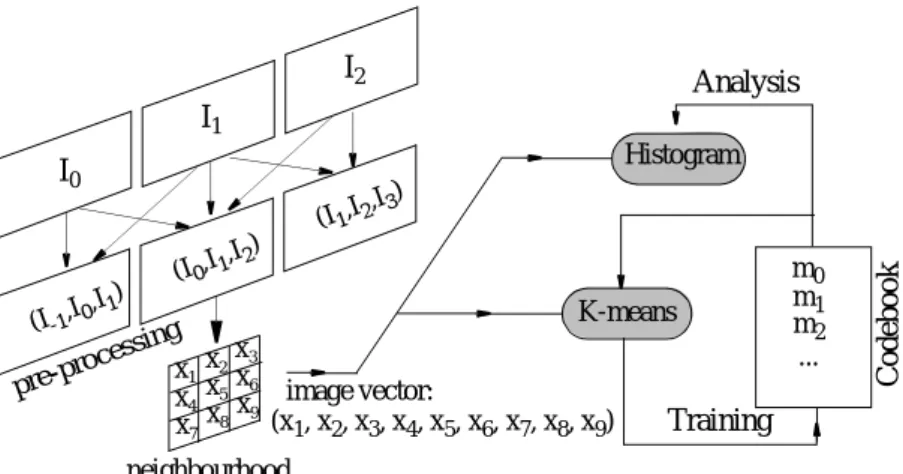
The clustering algorithm can be applied directly on the original image, but in order to give the algorithm some convenient invariance properties a preliminary image trans-formation should be useful. The overall process is illustrated in Fig. 1 where the pre-processing step is represented with the spatio-temporal function .

k

=

n

×

n

mk

m

As we are more particularly concerned with invariance to lightning change, we pro-pose an implementation in which the output of the pre-processing step represents the image gradient arguments. We suggest to code the resulting image data with 16 values, which means a quantization step. When considering colour images, only the argument of the gradient which have the maximal magnitude (computed as in [11]) is kept, if this magnitude is above a given threshold.

2.3 Distance function

Whether being concerned with the training step or with the analysis step, the vectors extracted from an image have to be compared to those gathered in the dictionary. The metric to use depends on whether or not the image has been pre-processed.

Referring to an original image, we propose this metric to be represented by the Euclid-ian distance between the two vectors after they have been normalized. Let us assume that and are the two normalized vectors to compare, the distance between these vectors is given by:

As this metric is representative of the angle and does not consider the vector modulus, it is supposed to be invariant to illumination changes. The algorithm elaborated with this metric will be denoted algorithm 1 afterwards.

The alternative technique we propose to apply consists in pre-processing the original image in order to make each of the vector components invariant to illumination changes. So, we propose that this step comes down to replace each pixel by a represen-tation of the argument of the gradient. In order to keep only the significant values, only the pixels whose gradient is above a given threshold are considered.

I₀ I₁ I₂ Ψ(I1,I2,I3 ) Ψ(I0,I1,I2 ) Ψ(I-1,I0,I1 ) K-means Histogram m₀ m₁ m₂ ... Training Analysis Co debo ok pre-pro cessing neighbourhood

Figure 1: Overall principle of the algorithm (with k=9).

image vector: (x₁, x₂, x₃, x₄, x₅, x₆, x₇, x₈, x₉) x1x2 x3 x4x5 x6 x7x8 x9

π 4

⁄

x

y

E

=

(

x

₁

–

y

₁

)

2

+

(

x

₂

–

y

₂

)

2

+

…

+

(

x

_N

–

y

_N

)

2

4. A quantization step of leads us to get a 16-value code that have to be completed with an additional value to code the non-significant data. Regardless to the original image the resulting data are reduced and a simple distance can be elaborated to com-pare two vectors. We propose to use the following one, based on the L1 norm:

where and are respectively the th component of the two vectors to compare. The algorithm elaborated with this metric will be denoted algorithm 2 afterwards.

3

Histogram comparison

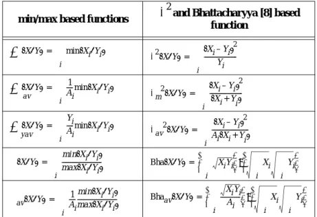
The analysis step consists in searching for every image neighbourhood, the nearest vector in the codebook. The various results enable either to quantize the original image or to implement an efficient histogram algorithm. At the end of this step, any image is supposed to be characterized by a single histogram and so comparing the obtained his-tograms between them should indicate how much the corresponding images are simi-lar. This section addresses this problem of histogram comparison through a brief presentation of a few possible comparison functions drawn from statistics, signal processing and geometry. Table 1 gives expressions for such convenient functions, most of them found in the literature, by dividing them into two groups according to their origin. In this table, we assume the vectors and represent the two histo-grams to be compared, and the vector A is an average histogram as far as such a piece of information is available.

Table 1: Distance functions considered for histogram comparison.

min/max based functions and Bhattacharyya [8] based

function

π 4

⁄

E

=

α

₁

–

β

₁

+

α

₂

–

β

₂

+

…

+

α

_N

–

β

_N

α

_i

β

_i

i

X

Y

χ

2 X Y, ( )

∩

min X( _i,Y_i) i

∑

= χ2(X Y, ) (Xi–Yi) 2 Y_i ---i

∑

= X Y, ( ) av

∩

1 A_i --- min X( _i,Y_i) i

∑

= χ_m2(X Y, ) X_i–Y_i ( )2 X_i+Y i ( ) ---i

∑

= X Y, ( ) yav

∩

Yi A_i --- min X( _i,Y_i) i

∑

= _χ av 2 X Y, ( ) (Xi–Yi) 2 A_i(X_i+Y_i) ---i

∑

= Ψ X Y( , ) min X( i,Yi) m ax X( _i,Y_i) ---i

∑

= Bha X Y( , ) X_iY_i i

∑

⎝ ⎠ ⎜ ⎟ ⎛ ⎞ X_i i

∑

Y_i i

∑

⎝ ⎠ ⎜ ⎟ ⎛ ⎞ ⁄ = Ψ_av(X Y, ) 1 A_i ---min X( i,Yi) ma x X( _i,Y_i) ---i

∑

= Bhaav(X Y, ) X_iY_i A_i ---i

∑

⎝ ⎠ ⎜ ⎟ ⎛ ⎞ X_i i

∑

Y_i i

∑

⎝ ⎠ ⎜ ⎟ ⎛ ⎞ ⁄ =

4

Application to place recognition

The experiments have been conducted on the INDECS database [9][10], which con-tains pictures of five different rooms acquired at different times of the day under dif-ferent viewpoints and locations. The system is trained for all the pictures acquired under a given illumination condition and tested under the other illumination conditions for the remaining pictures. For a given picture, the aim is to recognize the room in which it has been acquired.

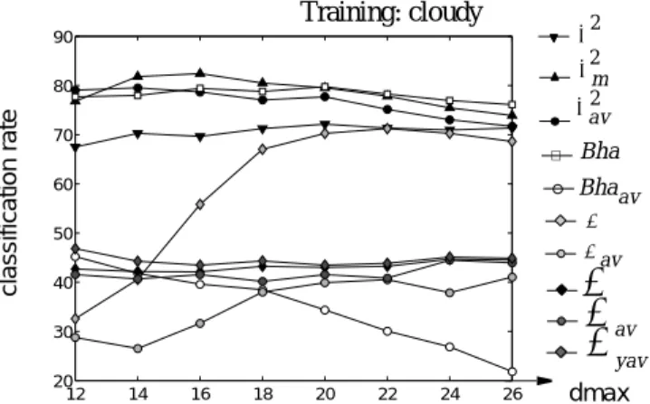
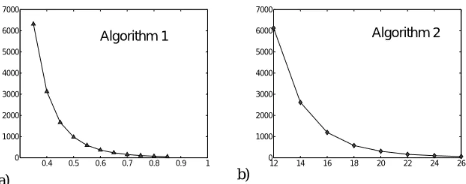
The first tests have been done with our two algorithms in order to evaluate the different distance functions used for histogram comparison. They consist to evaluate the classi-fication rate (that is the successful room recognition rate) for every image of the data-base, giving each image the same weight. For better comparison with the results obtained in [9] (where the pictures containing less than 5 interest points were rejected) we choose to discard the images whose histogram contains no bin. This concerns about 1% of the total number of images. The results are plotted on figure 2 and figure 3. They indicate that the best results are obtained with Bhattacharyya metric when we consider algorithm 1 and the metric when we consider algorithm 2. Using this last metric, the classification rate of algorithm 2 are around 80% and the best rate is 82.42% with . The performance of algorithm 1 are weaker, but this per-formance increases when decreases. However, the evaluation has not been done for inferior to 0.35 as for this value the algorithm 1 has a great number of clusters (6 319 clusters) and consequently becomes too slow. Figures 4a and 4b illus-trates the swift variation of the number of clusters when dmax decreases, for both algo-rithms. χ_m2

dmax

=

16

dmax

dmax

12 14 16 18 20 22 24 26 20 30 40 50 60 70 80 90 dmax cl as si fic a ti on r a te

Figure 3: Global place classification rate using algorithm 2. Training: cloudy χ2_m χ2 χ_av2 Bha Bha_av ψ ψ_av av y av

∩

∩

∩

6.

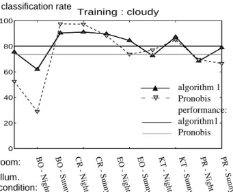
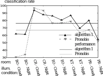
The classification rate is then calculated separately for each room and according to [9] a single measure of performance is computed by averaging all the results with equal weights. These results are plotted on figure 5 to figure 7, with regard to the results obtained in [9] and [10] which use a local feature detector constructed from the combi-nation of the Harris-Laplace detector and the SIFT descriptor. These figures clearly indicate that the performance measure obtained with our algorithm is the best, regard-less of which training set is chosen.

5

Conclusion

This study has tackled the image characterization problem by proposing a new approach based on a statistical analysis. Though this approach is very simple, it has been proven to be efficient and it has been empirically validated in the robotic frame-work of place recognition. Studies are in progress in order to improve the classification rates (splitting of the image into small regions, higher order statistic reduction) or to lead to real-time implementations of the proposed method.

0.4 0.5 0.6 0.7 0.8 0.9 1 25 30 35 40 45 50 55 60 65 70

Figure 2: Global place classification rate using algorithm 1.

cl as si fic a ti on r a te dmax y av Training: cloudy χ_m2 χ2 χ_av2 Bha Bha_av ψ ψ_av av

∩

∩

∩

0.4 0.5 0.6 0.7 0.8 0.9 1 0 1000 2000 3000 4000 5000 6000 7000 12 14 16 18 20 22 24 26 0 1000 2000 3000 4000 5000 6000 7000

Figure 4: Number of clusters with regard to the radius dmax.

Algorithm 1 Algorithm 2

Acknowledgments

The authors thank Maurice Diamantini for his contribution in programming with Ruby. This work was sponsored by the DGA. The support is gratefully acknowledged.

0 20 40 60 80 100 Training : cloudy B O - _N ig h_t B O - _S u_n n_y C R - _N ig_h t C R - _S u_n n_y E O - _N ig_h t E O - _S u_n n_y K T - _N ig_h t K T - _S u_n n_y P R - _N ig_h t P R - _S u_n n_y

Figure 5: Classification rates and performance measure after training the algorithm with "cloudy" illumination condition.

algorithm 1 Pronobis performance: algorithm1 Pronobis room: illum. condition: classification rate 20 30 40 50 60 70 80 90 100 B O - _C lo_u d_y B O - _S u_n n_y C R - _C lo_u d_y C R - _S u_n n_y E O - _C lo_u d_y E O - _S u_n n_y K T - _C lo_u d_y K T - _S u_n n_y P R - _C lo_u d_y P R - _S u_n n_y

Figure 6: Classification rates and performance measure after training the algorithm with "nighty" illumination condition.

algorithm 1 Pronobis performance: algorithm1 Pronobis room: illum. condition: classification rate

8.

References

[1] H. Wang and M. Brady, "Real-time corner detection algorithm for motion estimation," Im-age and Vision Computing 13 (9), pp. 695–703, 1995.

[2] C. Harris and M. Stephens, "A combined corner and edge detector," Proceeding of the 4th Alvey Vision Conference, pp. 147-151, 1988.

[3] M. Trajkovic and M. Hedley, "Fast corner detection". Image and Vision Computing 16 (2), pp. 75–87, 1998.

[4] K. Mikolajczyk et C. Schmid, "A performance evaluation of local descriptors, " IEEE Transactions on Pattern Analysis and Machine Intelligence, 27(10), pp. 1615-1630, 2005. [5] Y. Caron, H. Charpentier, P. Makris et N. Vincent, "Une mesure de complexité pour la

dé-tection de la zone d'intérêt d'une image," DGCI 2003.

[6] X. Feng, M. Pietikäinen et A. Hadid, "Facial Expression Recognition Based on Local Bi-nary Pattern," Pattern Recognition and Image Analysis, Vol. 17, No.4, (2007), 592-598. [7] M. Varma and A. Zisserman, "A Statistical Approach to Material Classification Using

Im-age Patch Exemplars, " to be published in IEEE PAMI .

[8] N. A. Thacker, F. J. Aherne and P. I. Rockett, "The Bhattacharyya Metric as an Absolute Similarity Measure for Frequency Coded Data," Kybernetika, Prague 9-11 June, 1997. [9] A. Pronobis, "Indoor Place Recognition Using Support Vector Machines," Master’s Thesis

in Computer Science, 2005.

[10] A. Pronobis, B. Caputo, P. Jensfelt and H. I. Christensen, "IA Discriminative Approach to Robust Place Recognition," ICIRS, Beijing, China, 2006.

[11] S. D. Zenzo, "A note on the Gradient of a multi-image," CVGIP, 33, pp 116-125, 1986.

30 40 50 60 70 80 90 100 B O - _C lo_u d_y B O - _N ig_h t C R - _C lo_u d_y C R - _N ig_h t E O - _C lo_u d_y E O - _N ig_h t K T - _C lo_u d_y K T - _N ig_h t P_R - _C lo_u d_y P_R - _N ig_h t

Figure 7: Classification rates and performance measure after training the algorithm with "sunny" illumination condition.

algorithm 1 Pronobis performance: algorithm 1 Pronobis room: illum. condition: classification rate