HAL Id: inria-00346540
https://hal.inria.fr/inria-00346540
Submitted on 11 Dec 2008
HAL is a multi-disciplinary open access
archive for the deposit and dissemination of
sci-entific research documents, whether they are
pub-lished or not. The documents may come from
teaching and research institutions in France or
L’archive ouverte pluridisciplinaire HAL, est
destinée au dépôt et à la diffusion de documents
scientifiques de niveau recherche, publiés ou non,
émanant des établissements d’enseignement et de
recherche français ou étrangers, des laboratoires
Query Results
Mounir Bechchi, Amenel Voglozin, Guillaume Raschia, Noureddine Mouaddib
To cite this version:
Mounir Bechchi, Amenel Voglozin, Guillaume Raschia, Noureddine Mouaddib. Multi-Dimensional
Grid-Based Clustering of Fuzzy Query Results. [Research Report] RR-6770, INRIA. 2008, pp.29.
�inria-00346540�
a p p o r t
d e r e c h e r c h e
0249-6399 ISRN INRIA/RR--6770--FR+ENG Thème SYMMulti-Dimensional Grid-Based Clustering of Fuzzy
Query Results
Mounir Bechchi — Amenel Voglozin — Guillaume Raschia — Noureddine Mouaddib
N° 6770
Centre de recherche INRIA Rennes – Bretagne Atlantique
Mounir Bechchi
∗, Amenel Voglozin
∗, Guillaume Raschia
∗,
Noureddine Mouaddib
†Thème SYM — Systèmes symboliques Équipe-Projet Atlas
Rapport de recherche n° 6770 — 2008 — 26 pages
Abstract: In usual retrieval processes within large databases, the user formu-lates a first basic (broad) query to target and filter data and next, she starts browsing the answer looking for precise information. We then propose to per-form an offline hierarchical grid-based clustering of the data set in order to quickly provide the user with concise, useful and structured answers as a start-ing point for an online exploration. Every sstart-ingle answer item describes a subset of the queried data in a user-friendly form using linguistic labels, that is to say it represents a concept that exists within the data. Moreover, answers of a given ‘blind’ query are nodes of a classification tree and every subtree rooted by an answer offers a ‘guided tour’ of a data subset to the user. Finally, an experi-mental study shows that our process is efficient in terms of computational time and achieves high quality clustering schemas of query results
Key-words: Database Summary, Flexible Query, Clustering of Query Results
∗Atlas-Grim,INRIA/LINA-Université de Nantes †Université Internationale de Rabat
Résumé : Actuellement, la maturité des SGBDs et leur utilisation inten-sive dans les systèmes d’information a eu, entre autres, une conséquence ma-jeure dans les entreprises : la production de bases de données volumineuses. La masse d’information ainsi obtenue est difficilement exploitable. En effet, les utilisateurs de ces systèmes doivent faire face au problème de ‘surcharge d’information’ lors de l’interrogation de leurs données, qui se traduit par un nombre de réponses trop élevé à des requêtes exploratoires. L’organisation et le filtrage de l’information en fonction de l’utilisateur et de la requête est un moyen privilégié pour résoudre ce problème. L’approche proposée dans ces travaux con-siste à regrouper les réponses à une requête utilisateur en un ensemble de classes (ou résumés) organisées hiérarchiquement. Chaque classe décrit un ensemble de n-uplets dont les propriétés sont voisines. L’utilisateur pourra ainsi explorer la hiérarchie pour localiser les n-uplets qui l’intéressent et en écarter les autres. Le principe cognitif mis en oeuvre dans cette approche est que les réponses perti-nentes sont a priori semblables et donc appartiennent à la même classe d’objets homogènes. Notre algorithme d’interrogation utilise une hiérarchie de résumés (une hiérarchie SaintEtiQ) pré-calculé sur l’ensemble des données pour fournir une classification hiérarchique (collection de résumés) comme réponse à une re-quête utilisateur. Ainsi, il améliore l’analyse exploratoire par la construction de réponses plus générales, moins nombreuses et mieux ciblées.
Mots-clés : Résumé de données, Requêtes flexibles, Classification des résul-tats d’une requête
1 Introduction
Because of the ever increasing amount of information stored each day into databases, user can no longer have an exploratory approach for visualizing, querying and analyzing their data without facing the dual issues of Empty and Many answers. In the former case, very few tuples or even no tuples satisfy the user’s query, while in the latter, the user is provided with too many tuples forc-ing her to spend unnecessary time siftforc-ing through these items to find relevant results. This is due to the fact that traditional database query processing mod-els have always assumed that the user knows what she wants and consequently tuples that exactly satisfy the selection conditions in the query are returned, no more and no less.
The empty answers problem happens when the user submits a very restrictive query. Many approaches, based for instance on query relaxation [1] or nearest-neighbor [2] techniques, are proposed to address such problem. These techniques allow the database system to retrieve tuples that closely (though not completely) match the user’s query. We do not consider the empty answers problem in this paper.
In contrast, the user faces the so-called many answers (or information over-load) problem when she submits a ‘broad’ query, i.e. , she has a vague and poorly defined information need. Means to circumvent such problem include query-by-example [3] [4] and ranking [5] [6] based techniques. Such techniques first seek to approximate user’s requirement. For instance, systems proposed in [3] [4] use relevance feedback from the user (few records judged to be relevant by the user) while works in [5] [6] use past behavior of the user (derived from available workloads). Then, they compute a score (similarity measures) of ev-ery answer that represents the extent to which it is relevant to the estimated user’s requirement. Finally, the user is provided with a ranked list, in descend-ing order of relevance, of either all query results or only the top-k [7] subset. The effectiveness of the above approaches depends on their ability to accurately capture the user’s requirement, which is, unfortunately, a very difficult and time consuming task.
In this communication, we adopt a completely different strategy to handle many answers problem. It consists in dividing the answer tuples set into different groups, allowing the user to select and browse groups that most closely match what she is looking for, ignoring the irrelevant ones. Indeed, such technique focuses on the user’s participation in a cycle of query refinement instead of trying to understand and estimate the user’s needs. This idea has traditionally been used for organizing the results of Web search engines [8] [9] [10] [11] but has only recently been used in the context of relational database [12] [13] [14] (see Section 2). However, these approaches are performed on query results and consequently occur at query time. Thus, the overhead time cost is an open critical issue for such a posteriori tasks.
To address this issue, we propose to perform an offline hierarchical grid-based clustering of the whole data set in order to quickly provide the user with concise, useful and structured answers as a starting point for an online analysis. Each answer item describes a subset of the queried data in a human-readable form using linguistic labels. Moreover, answers of a given ‘blind’ query are nodes of the clustering tree and every subtree rooted by an answer offers a ‘guided tour’ of a data subset to the user. Organizing tuples in nested clusters reduces the
‘information overload’, allowing the user to spend less time sifting and sorting through the results in order to retrieve the required piece of information. The leading idea of this proposal is the Cluster Hypothesis [8]: closely associated items tend to be relevant to the same request. However, since such hierarchical grid-based clustering is independent of the query, the set of starting point an-swers could be large and consequently dissimilarity between items is susceptible to skew. It occurs when the pre-computed clustering schema is not perfectly adapted to the user query. To tackle this problem, we propose an efficient and effective algorithm that rearranges answers based on the hierarchical structure of the pre-computed clustering schema, i.e. , no clustering at all would have to be performed at query time.
The rest of the paper is organized as follows. First, we describe works that relate to our proposal (Section 2). In Section 3 we detail the underlying clustering technique coined SaintEtiQ we consider in this work. Then, in Section 4 we present a querying mechanism to efficiently access SaintEtiQ outputs and we discuss how summary results help facing many answers problem. An algorithm that addresses the problem of cluster dissimilarity by rearranging query results is presented in Section 5. Section 6 discusses an extension of the above process that allows every user to use her own vocabulary when querying the database. An experimental study using real data is presented in Section 7. Finally we give a conclusion and future directions of that work in Section 8.
2 Related work
Clustering of query results has been extensively investigated in areas outside database research such as Information Retrieval. The idea was first introduced in the Scatter/Gather system [8], which is based on a variant of the classical K-Means algorithm. It performs clustering of the results after the documents matching the query have been identified by the search engine. Since then, several classes of algorithms have been proposed (SHOC [9], EigenCluster [10], SnakeT [11]). Such post-processing algorithms introduce a noticeable overhead time cost to the query processing, due to the large number of results returned by the search engine. However, they testify that there is a significant potential benefit in providing additional structure in large answer sets.
In contrast to the internet text search, clustering of query results have re-ceived much less attention in the database field. An automatic method for cat-egorizing query results (instead of clustering) is proposed in [12]. It performs categorization as post-processing after query results are obtained, with the focus on minimizing the user navigation cost. In [13], authors propose OSQR, an ap-proach for grouping query result based on agglomerative single-link clustering. Given an SQL query as input, OSQR identifies the set of keywords (or values) that occur frequently in the query’s result and then associates each result with a subset of keywords. Next, it clusters keywords based on a keywords distance function. The clustering of keywords, in turn, induces a clustering of the query result rows. In a recent work [14], authors generalize SQL group-by operator to enable fuzzy clustering of database query results on a set of attributes specified in the user’s input query. This approach uses a grid-based clustering method based on a variant of the classical K-Means algorithm and generates flat clus-tering of query results. Note that the number of clusters has to be provided as a
parameter in the query, which assumes that a priori knowledge about the data is available. All the above proposals provide the user with a higher-level view of the data and can be used for an easier navigation in the result. However, categorization and clustering of query results are performed at query time and imply an overhead cost in the query processing.
3 Overview of the SaintEtiQ System
In this section, we introduce the main ideas of SaintEtiQ [15], the grid-based clustering model we consider in this work. Then, we give useful definitions and properties regarding our proposal.
3.1 A Two-Step Process
SaintEtiQ takes tabular data as input and produces multi-resolution sum-maries of records through an online mapping and a summarization processes. 3.1.1 Mapping Service
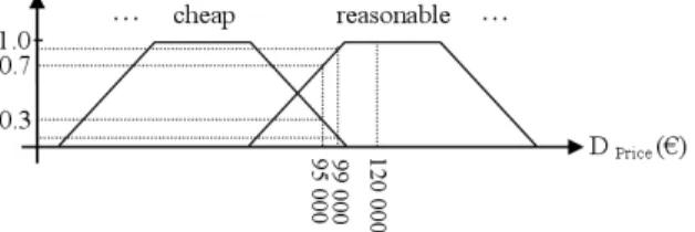
The SaintEtiQ system relies on Zadeh’s fuzzy set theory [16] and, more specifically on linguistic variables [17] and fuzzy partitions [18] to represent data in a concise form. The fuzzy set theory is used to translate records in accordance with a Knowledge Base (KB) provided by a domain expert or even a user. Basically, the operation replaces the original values of every record in the table by a set of linguistic descriptors defined in the KB. For instance, with a linguistic variable on attribute Price (Figure 1), a value t.Price = 95000e is mapped to {0.3/cheap, 0.7/reasonable} where 0.3 is a membership grade that tells how well the label cheap describes the value 95000. Extending this mapping to all the attributes of a relation could be seen as locating the cells in a grid-based multidimensional space that map records of the original table. The grid is defined by the KB and corresponds to the user’s perception of the data space.
Figure 1: Fuzzy linguistic partition defined on the attribute Price Thus, tuples t1, t2 and t3 in Table 1 are mapped into two distinct grid-cells
denoted by c1 and c2 in Table 2. old is a fuzzy label a priori provided by the
KB on attribute Age and it perfectly matches (with degree 1) range [19, 24] of raw values. Besides, tuple count column gives the proportion of records in R that belong to the cell and 0.3/cheap says that cheap fits the data only with a small degree (0.3). The degree is computed as the maximum of membership grades of tuple values to cheap in c1.
Table 1: Raw data R Id Age Price
t1 22 95000
t2 19 99000
t3 24 120000
Table 2: Grid-cells mapping Id Age Price tuple count c1 old 0.3/cheap 0.4
c2 old reasonable 2.6
Flexibility in the vocabulary definition of KB permits to express any single value with more than one fuzzy descriptor and avoid threshold effect due to a smooth transition between two descriptors. Besides, KB leads to the point where tuples become indistinguishable and then are grouped into grid-cells such that there are finally many more records than cells. Every new (coarser) tu-ple stores a record count and attribute-dependant measures (min, max, mean, standard deviation, etc.). It is then called a summary.
3.1.2 Summarization Service
Summarization service is the last and the most sophisticated step of the Sain-tEtiQ system. It takes grid-cells as input and outputs a collection of sum-maries hierarchically arranged from the most generalized one (the root) to the most specialized ones (the leaves). Summaries are clusters of grid-cells, defining hyperrectangles in the multidimensional space. In the basic process, leaves are grid-cells themselves and the clustering task is performed on K cells rather than N tuples (K << N). From the mapping step, cells are introduced continuously in the hierarchy with a top-down approach inspired of D.H. Fisher’s Cobweb, a conceptual clustering algorithm [19]. Then, they are incorporated into best fitting nodes descending the tree. Three more operators could be applied, de-pending on partition’s score U, that are create, merge and split nodes. They allow developing the tree and updating its current state. U is a combination of two well-known measures: typicality [20] and contrast [21]. Those measures maximize within-summary similarity and between-summary dissimilarity. Fig-ure 2 represents the summary hierarchy built from the cells c1 and c2.
3.2 Features of Summaries
We introduce in this section basic definitions related to the SaintEtiQ sum-marization process.
Definition 1 Summary. Let E = !A1, . . . , An" be an n-dimensional space
equipped with a fuzzy grid that defines basic n-dimensional overlapping areas called cells in E. Let R be a relation defined on the cartesian product of domains DAi of dimensions Ai in E. Summary z of relation R is the bounding box of
the cluster of cells populated by records of R.
The above definition is constructive since it proposes to build generalized summaries (hyperrectangles) from cells that are specialized ones. In fact, it is equivalent to performing an addition on cells:
z = c1+ c2+ . . . + cp
where ci∈ Lz, the set of p cells (summaries) covered by z.
A summary z is then an intensional description associated with a set of tuples Rzas its extent and a set of cells Lzthat are populated by records of Rz.
Thus, summaries are areas of E with hyperrectangle shapes provided by the KB. From another point of view, they are nodes of the summary tree built by the SaintEtiQ system.
Definition 2 Summary Tree A summary tree over R is a collection Z of summaries verifying:
• ∀z, z!∈ Z, z! z! ⇐⇒ R
z ⊆ Rz!;
• ∃! z ∈ Z such that Rz= !z!∈ZRz!.
The relation over Z (i.e. , !) provides a generalization-specialization rela-tionship between summaries. And assuming summaries are hyperrectangles in a multidimensional space, the partial ordering defines nested summaries from the larger one to single cells themselves.
Finally, to determine a small set of data representing the whole data set, we need to extract a subset of summaries in the tree. The straightforward way of performing such a task is to define a summary partitioning.
Definition 3 Summary Partitioning. The set P of leaves of every rooted sub-tree of the summary hierarchy provides a partitioning of relation R.
We denote by Pz the top-level partition of z in the summary tree. It is
then the most general partitioning of Rz we can provide from the tree. Note
that the most specialized partitioning is the set of cells covering Rz, that is Lz.
A partitioning can be obtained a posteriori to set the compression rate from the user’s needs. For instance, general trends in the data could be identified in the very first levels of the tree whereas precise information has to be looked at near the leaves. Moreover, such a partitioning verifies two basic properties: disjunction and coverage.
Property 1 Disjunction
Regarding such a property, summaries of a partition do not overlap with each other, if we except overlapping of borders of fuzzy cells.
Property 2 Coverage
R =∪z∈PRz
A partition P ensures coverage of the whole data set R since, by definition, representatives of every branch are included into P.
3.3 Discussion about SaintEtiQ
The use of SaintEtiQ instead of any other clustering approaches [22] offers a number of advantages. The produced summary hierarchy provides multidi-mensional views on the data at different levels of granularity through perfectly understandable high-level descriptors. Thus, the user can determine at a glance whether a cluster’s content is of interest. Furthermore, SaintEtiQ applies a conceptual clustering algorithm for partitioning the incoming data in an incre-mental and dynamic way. Thus, changes in the database are reflected through such incremental maintenance of the complete hierarchy (see [15]). Of course, for each application, experts have to be consulted to create linguistic labels as well as the fuzzy-logic membership functions. However, it is worth noticing that, once such knowledge base is defined, the system is fully autonomous with no human intervention required.
As on can observe, the SaintEtiQ hierarchy acts as a multidimensional index. Indexes based on tree structures are widely used for organizing and accelerating access to large multidimensional data sets. The most popular is R-Tree [23] and its variants aR-R-Tree [24], aP-R-Tree [25]. R-R-Tree-based approaches partition the data domain into buckets (i.e. , intervals in several dimensions) and build a height-balanced tree that represents the data as nested structured buckets of increasing resolution. Each leaf node is a bucket containing at most M pointers to the tuples it covers and each inner node contains at most M pointer to a lower nodes in the tree structure. M is an input parameter which depends on the hard disk drive’s properties (capacity and sector size). Theses approaches, even though they are very efficient for multidimensional data querying, are not very useful in the context of data discovery, analysis and exploration. Indeed, the grid (buckets) depends on the distribution of the record values rather than the user’s perception of the domain. Furthermore, the grouping process depends on the parameter M and consequently tuples within each group do not meet the cluster hypothesis “closely associated tuples tend to be relevant to the same query”.
In the next section, we present a querying mechanism for users to efficiently access the hierarchical summaries produced by SaintEtiQ . Then, we discuss how summary answers reduce information overload that user experiences when querying large databases.
4 Querying the SaintEtiQ Summaries
Database systems are being increasingly used for interactive and exploratory data retrieval; examples include users searching their favorite houses, cars, movies, restaurants, and so on over the web. In this context, the user often
has not a specific retrieval goal and is interested in browsing through a set of items (to explore what choices are available) instead of searching among them. For instance, imagine a user who is looking for a house in a database of homes for sale, consisting of a single relation R with attributes Price, Age, Location. The typical facility available to her is Boolean SQL queries. In terms of query semantics, the user is limited by hard query conditions or constraints (e.g. , Price ∈ [150ke, 250ke]). However, in many situations, the user actually may not have such hard constraints clearly in her mind. Sometimes it is even im-possible to come up with such constraints without knowing what the database contains in the first place. In terms of result organization, what the user gets is a flat table of query results that exactly satisfy all the constraints of the query and thus are equally relevant to the query. While extremely useful for the expert user, the Boolean retrieval model is inadequate for ad-hoc retrieval by exploratory users who cannot articulate the perfect query for their needs -there is usually too many query results returned for a submitted query forcing the user to spend unnecessary time sifting through these items to find relevant results.
To address this problem, we propose a fuzzy retrieval system that (1) uses the SaintEtiQ hierarchy instead of the database to access data; (2) allows users to express vague requirements instead of crisp ones thanks to linguistic labels defined on each attribute domain in the KB; (3) provides users with useful and structured answers as a starting point for an exploratory analysis. However, choosing the fuzzy labels from a controlled vocabulary compels the user to adopt a predefined categorization materialized by the fuzzy cells. In Section 6, we deal with user-specific linguistic labels to overcome this pitfall.
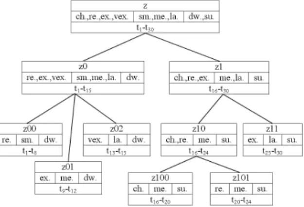
To illustrate our proposal, we introduce here a sample data set R with 30 records (t1− t30) represented on three attributes: Price, Size and Location.
We suppose that {cheap (ch.), reasonable (re.), expensive (ex.), very expensive (vex.)}, {small (sm.), medium (me.), large (la.)} and {downtown (dw.), sub-urb (su.)} are sets of linguistic labels defined respectively on attributes Price, Size and Location. Figure 3 shows the summary hierarchy HR provided by
SaintEtiQ performed on R.
4.1 Expression and Evaluation of a Query
The fuzzy querying mechanism proposed here intends to evaluate queries such as Q1:
Example 1 Q1: SELECT * FROM R WHERE Location IN {suburb} AND Size IN {medium OR large}.
The interpretation we adopted is such that queries are under a conjunc-tive form: modalities on an attribute are connected with an OR operator and attributes are connected with an AND operator. The AND operator is used be-cause the process should select only data that comply with the characterization on both Location and Size. On the other hand, the use of the OR operator is due to data constraint: database records are single-valued tuples.
In the following, we denote by X the set of attributes specified in the user’s input query and Y the set of missing attributes which is the complement of X relatively to R: X ∪ Y = R and X ∩ Y = ∅. Further, for each attribute A ∈ X, QAdenotes the set of fuzzy labels (called required features) defined on attribute
A. The set of sets QA is denoted by QX (see example 2).
Example 2 Consider query Q1 stated above. We have X ={Location, Size}, Y ={Price}, QLocation={suburb}, QSize={medium,large} and QX ={QLocation
,QSize}.
Let LA(z) be the set of descriptors that appear in a summary z on attribute
A. When confronting z with a query Q to decide whether it corresponds to that query and can then be considered as a result, three cases might occur:
a: no correspondence (i.e. , ∃A ∈ X, LA(z) ∩ QA = ∅). For one attribute
or more, z has no required feature, i.e. , it shows none of the descriptors mentioned in query Q.
b: exact correspondence (i.e. , ∀A ∈ X, LA(z) ⊆ QA). The summary z
matches the query Q semantics. It is considered as a result.
c: no decision can be made (i.e. , ∃A ∈ X, LA(z) − QA-= ∅). There is one
attribute A for which z exhibits one or many descriptors besides those strictly required (i.e. , those in QA). Presence of required features in
each attribute of z suggests, but does not guarantee, that results may be found in the subtree rooted by z. Exploration of the subtree is necessary to retrieve possible results: for each branch, it will end up in situations categorized by case a or case b. Thus, at worst at leaf level, an exploration leads to accepting or rejecting summaries; the problem of indecision is always solved.
The situations stated above reflect a global view of the confrontation of a summary z with a query Q.
4.2 Search algorithm
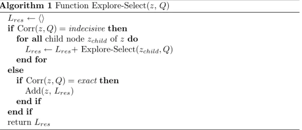
The Explore-Select Algorithm (ESA) applies the above matching procedure over the whole set of summaries, organized in a hierarchy, to select relevant summaries. Since the selection should take into account all summaries that
correspond to the query, exploration of the hierarchy is complete. Algorithm 1 describes the ESA algorithm with the following assumptions:
• the function returns a list of summaries;
• function Corr symbolizes the matching test reported in Section 4.1; • operator ‘+’ performs a list concatenation of its arguments;
• function Add is the classical constructor for lists, it adds an element to a list of the suitable type;
• Lres is a local variable.
Algorithm 1 Function Explore-Select(z, Q) Lres ← !"
if Corr(z, Q) = indecisive then for all child node zchildof z do
Lres← Lres+ Explore-Select(zchild, Q)
end for else
if Corr(z, Q) = exact then Add(z, Lres)
end if end if return Lres
The ESA algorithm is based on a depth-first search and relies on a property of the hierarchy: the generalization step in the SaintEtiQ model guarantees that any descriptor that exists in a node of the tree also exists in each parent node. Inversely, a descriptor is absent from a summary’s intent if and only if it is absent from all subnodes of this summary. This property of the hierarchy permits branch cutting as soon as it is known that no result will be found. Depending on the query, only a part of the hierarchy is explored.
Thus, results of Q1 (Example 1), when querying the hierarchy shown in Figure 3, look like:
Table 3: Q1 results
Id_Sum Price Size Location z1 cheap reasonable expensive medium large suburb
In this case, the ESA algorithm first confronts z (root) with Q1. Since no decision can be made, Q1 is respectively confronted to z0 and z1, the children of z. The subtree rooted on z0 is then ignored because there is no correspondence between Q1 and z0. Finally z1 is returned because it exactly matches Q1. Thus, the process tests only 30% of the whole hierarchy.
Note that, the set of records Rz1covered by z1 can be returned
(SHOWTU-PLES operation) by simply transforming the intent of z1 into an SQL query qz1
and sending it as a usual query to the database system. The WHERE clause of qz1 is generated by transforming the fuzzy labels (vague criteria) contained
in the intent of z1 into crisp ones. In other words, each linguistic label l on an attribute A is replaced by its support, i.e. , the set of all values in DA
that belong to l with non-zero membership. Then, the obtained crisp criteria on each summary’s attribute are connected with OR operator and summary’s attributes are connected with AND operator to generate the WHERE clause. Thus, performing a SHOWTUPLES operation takes advantage of the optimiza-tion mechanisms that exist in the database system.
Furthermore, tuples covered by z1 can also be sorted, thanks to their sat-isfaction degrees to the user’s query, using an overall satsat-isfaction degree. We assign to each tuple the degree to which it satisfies the fuzzy criteria of the query. There are many propositions in the literature for defining aggregation connectives [26]. Usually, the minimum and maximum functions stand for the conjunctive and disjunctive connectives.
The ESA algorithm is particularly efficient. In the worst case (exploration of the hierarchy is complete), its cost is given by:
CESA(L) = ε ·
L− 1
w− 1 ∈ O(L)
where L is the number of leaves (cells) of the tree, w its average width and coefficient ε corresponds to the time required for confronting one summary in the hierarchy against the query.
4.3 Multi-Scale Summarized Answers
Given a fuzzy query Q, the ESA algorithm produces a set of clusters (summaries) from a SaintEtiQ hierarchy instead of a list of tuples tset(Q). Each answer item z describes a subset of the query result set tset(Q). Hence, the user can unambiguously determine whether Rz contains relevant tuples only by looking
at the intensional description of z and particulary on unspecified attributes (Y ) because all answer tuples satisfy the specified conditions related to attributes in X. Three cases might occur:
1: summary z doesn’t fit user’s need. It means that for at least one unspeci-fied attribute A ∈ Y , all linguistic labels (the set LA(z)) are irrelevant to
the user. For instance, consider the Q1 results (Table 3). z1 doesn’t con-tain any relevant tuple if the user is actually looking for very cheap homes because very cheap /∈ LP rice(z1). In other words, none of the records in
Rz1 is mapped to very cheap on attribute Price and consequently a new
broad query with less selective conditions may be submitted or the task may be abandoned (we denote this with the IGNORE option).
2: summary z exactly fits user’s need. It means that for each A ∈ Y , all linguistic labels in LA(z) are relevant to the user. Assume that the user is
interested in cheap, reasonable as well as expensive homes. Thus, all tuples contained in Rz1 are relevant to her. In such cases, she uses
SHOWTU-PLES option to access tuples stored in Rz. The SHOWTUPLES option
3: summary z partially fit user’s need. In this case, there is at least one attribute A ∈ Y for which LA(z) exhibits too many linguistic labels
re-garding the user’s requirement. For instance, the set Rz1partially matches
the needs of a user who is looking for cheap as well as reasonable homes be-cause Rz1contains also tuples that are mapped to expensive on attribute
Price. In this case, a new query with more selective conditions (e.g. , Price IN{cheap OR reasonable}) may be submitted or a new clustering schema of the set Rz, i.e. , which allows to examine more precisely the
dataset, is required. Since z is a hyperrectangle, we present to the user the children of z (SHOWCAT option). Each child of z represents only a portion of tuples in Rz and gives a more precise representation of tuples
it contains. For example, {z10,z11} partitions Rz1 into two subsets Rz10
and Rz11; z10exactly fit user needs. Since the entire tree is pre-computed,
no clustering at all would have to be performed at feedback time. The SHOWCAT option is similar to the one defined in [12].
More generally, a set of summaries S = {z1. . . zm} (clusters) is presented to
the user as a clustering schema of the query result tset(Q). The three options IGNORE (case 1), SHOWTUPLES (case 2) and SHOWCAT (case 3) give the user the ability to browse through the S structure (generally a set of rooted subtrees), exploring different datasets in the query results and looking for rel-evant information. Indeed, the user navigates through the set S = {z1. . . zm}
using the following exploration model:
i) start the exploration by examining the intensional description of zi ∈ S
(initially i = 0);
ii) if case 1, ignore zi and examine the next cluster in S, i.e. , zi+1;
iii) if case 2, navigate through tuples of Rzi to extract every relevant tuple
and thereafter, go ahead and examine zi+1;
iiii) if case 3, navigate through children of zi, i.e. , repeat from step (i) with S,
the set of children of zi. More precisely, examine the intensional
descrip-tion of each child of zi starting from the first one and recursively decide
to ignore it or examine it (SHOWTUPLES to extract relevant tuples or SHOWCAT option for further expansion). At the end of the exploration of the children of zi, go ahead and examine zi+1.
This process stops when the user reaches the relevant cluster, i.e. , the one that meets her requirement. Indeed, our general assumption is that relevant tuples for the same user’s requirement are more similar (close) to each other and consequently they belong to the same cluster at a given granularity level.
For instance, suppose a user is looking for medium, large as well as cheap homes but issues the query Q1 (Example in Section 1). The set of summaries S presented to such user is {z1} (Table 3), where z1 is a subtree in the pre-computed hierarchy shown in Figure 3. Thus, the user can explore the subtree rooted by z1 as follows to reach relevant tuples: analyze z1 intent and explore it using SHOWCAT option, analyze z10 intent and explore it using SHOWCAT option, analyze z110 intent and use SHOWTUPLES option to navigate through the tuples in Rz110 = t16− t20 and identify every relevant tuple, analyze z101
Note that when the set S = {z} is a singleton, i.e. , z is a node of the pre-computed clustering tree, its exploration is straightforward. Indeed, given a summary of the tree rooted by z the user wishes to examine more closely (SHOWCAT option), its children are well separated since SaintEtiQ is de-signed for converging to the locally optimized hierarchy. Furthermore, the num-ber of clusters presented to the user, at each time, is small; the highest value is equal to the maximum width of the pre-computed tree. However, S is often a set of summaries of the pre-computed tree. Since the hierarchical grid-based clustering schema is independent of the query, the size of S could be large and consequently, dissimilarity between its items is susceptible to skew. It occurs when the pre-computed clustering schema is not adapted to the user query. In such cases, choosing the relevant summaries from the large starting point results S is a difficult endeavor. In the following section, we describe an algorithm for rearranging query results.
5 Rearranging query results
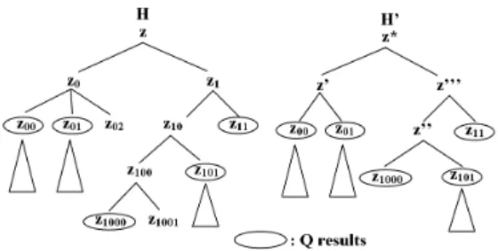
Consider the pre-computed hierarchy H shown in Figure 4 (Left) and a user’s query Q. Furthermore, suppose that the ESA algorithm returns the set of summaries S = {z00, z01, z1000, z101, z11} when querying H using Q. Results for
Q are scattered over the tree. Users often face the above problem since the hierarchical grid-based clustering is independent of the query.
Figure 4: (Left) A pre-computed hierarchy H (Right) Rearranging Q summary results
A straightforward way to address this problem would be to, first, execute SaintEtiQ summarization service (SEQ) on the cells populated by records of tset(Q). Then, we present to the user the top-level partition of the result tree. Thus, size reduction and discrimination between items in S are clearly achieved at the expense of an overhead computational cost. Indeed, the SEQ process time complexity is in O(L!· log(L!)) with L! the number of cells populated by
answer records:
CSEQ= k · logw!(L!) · L!
where w! is the average width of the result tree, log
w!(L!) an estimation of its
average depth and coefficient k corresponds to the time required for evaluating the quality of a partition Pz resulting from the incorporation of a new cell
into each of the children nodes of z as well as additional operations (splitting, merging and creating a new node: see Section 3.1.2).
Thus, the global cost CESA+SEQ(L) of such a post-processing algorithm
(including search-ESA and summarization-SEQ steps) is in O(L · log(L)) where L is the number of leaves of the pre-computed tree (L / L! since the query is
expected to be broad). This solution doesn’t fit querying process requirements (see Section 7), that is to quickly provide to the user concise and structured answers.
To tackle this problem, we propose an algorithm, called Explore-Select-Rearrange Algorithm (ESRA), that rearranges answers based on the hierar-chical structure of the pre-computed clustering schema. The main idea of this approach is rather simple. It starts from the summary partition S (a clustering schema of the query results) and produces a sequence of clustering schemas with a decreasing number of clusters at each step. Each clustering schema produced at each step results from the previous one by merging the ‘closest’ clusters into a single one. Similar clusters are identified thanks to the hierarchical structure of the pre-computed clustering schema. Intuitively, summaries which are closely related have a common ancestor lower in the hierarchy, whereas the common ancestor of unrelated summaries is near the root. This process stops when it reaches a single hyperrectangle (the root z!). Then, we present to the user the
top-level partition (i.e. , children of z!) in the obtained tree instead of S.
For instance, when the ESRA process is performed on the set of summaries S ={z00, z01, z1000, z101, z11} stated above, the following sequence of clustering
schemas is produced:
z00 z01 z1000 z101 z11
z00+ z01 z1000+ z101 z11
z00+ z01 z1000+ z101+ z11
z00+ z01+ z1000+ z101+ z11
The hierarchy H!obtained from the set of query results S is shown in Figure 4
(Right) where z! = z
0− z02, z!! = z10 − z1001 and z!!! = z1− z1001. Thus,
the partition {z!, z!!!} is presented to the user instead of S. This partition
has a small size and defines well separated clusters. Indeed, all agglomerative methods, among them the ESRA algorithm, have a monotonicity property: the dissimilarity between the merged clusters is monotonically increasing with the level. It means, the dissimilarity value of the partition {z!, z!!!} is greater than
the dissimilarity value of the partition {z00, z01, z1000, z101, z11}.
Algorithm 2 describes the ESRA process. It is a modified version of algo-rithm 1 with the following new assumptions:
• it returns a summary (z!) rather than a list of summaries;
• function AddChild appends a node to caller’s children;
• function NumberofChildren returns the number of caller’s children; • function uniqueChild returns the unique child of the caller;
• function BuildIntent builds caller’s intent (hyperrectangles) from intents of its children;
Algorithm 2 Function Explore-Select-Rearrange(z, Q) Zres← Null
Z! ← Null
if Corr(z, Q) = indecisive then for all child node zchild of z do
Z! ← Explore − Select − Rearrange(z
child, Q) if Z!-= Null then Zres.addChild (Z!) end if end for if Zres.NumberofChildren() > 1 then Zres.BuildIntent() else Zres ← Zres.uniqueChild() end if else
if Corr(z, Q) = exact then Zres← z
end if end if return Zres
This ESRA process (Algorithm 2) returns a summary tree instead of a sum-mary list (Algorithm 1). Such sumsum-mary tree is built at the same time the pre-computed clustering schema is being scanned. It means that no clustering at all would have to be performed at query time. Hence, the computational complexity of the ESRA algorithm is in the same order of magnitude (i.e. , O(L)) than the ESA Algorithm (see Section 4.2):
CESRA(L) = (γ + ε) ·
L− 1 w− 1
where coefficient γ is the time cost for the additional operations (i.e. , addChild, uniqueChild and BuildIntent).
The ESRA cost is only a small constant factor γ larger than that of the ESA algorithm since ESRA algorithm takes advantage of the hierarchical structure of the SaintEtiQ summaries to merge similar clusters. However, a limitation relies in the fact that ESRA algorithm restrains the user to queries using a controlled vocabulary (i.e. , a summary vocabulary). Indeed, consider a user looking for cheap homes. What is meant by cheap can vary from one user to another one, or from one kind of users to another one (e.g. , cheap does not have the same meaning for home buyers and for apartment tenants). In the following, we deal with user-specific linguistic labels to overcome this problem.
6 Discussion about Extension to any Fuzzy
Predic-ate
We aim at allowing the user to formulate conditions in selection queries in her own language. As mentioned above, our current querying process cannot handle
free vocabulary. Regarding the query cost and accuracy, the ideal solution to address such problem consists in building a summary tree for every user such that queries and summaries share the same vocabulary (the grid). Thus, the ESRA algorithm, described in Section 5, can be used in its current state. But maintaining user-specific summaries is hardly conceivable in a system with multiple users. Two alternatives are then envisaged.
One could consider group profiles in order to reduce the number of man-aged summaries (e.g. , one for buyers and the other for tenants). In this case, the ESRA Algorithm can also be used directly since users formulate queries within the vocabulary of their groups. In this approach, users would subscribe to groups that share the same (or similar) vocabulary as theirs. In addition, they have to be familiar with their group’s terms before using them accurately. But this option is not much more convenient than using ad-hoc fuzzy labels, predetermined by a domain expert or even the database administrator. More-over, it only transposes the problem of user-specific summaries maintenance to group-specific ones.
Probably the most interesting solution consists in building only one SaintE-tiQ summary tree using an ad-hoc vocabulary, and querying these summaries with user-specific fuzzy labels. In the following, we assume that one summary tree of the database is considered. It is created using a priori defined linguis-tic variables that constitute the summary vocabulary. Nevertheless, the user defines her own fuzzy labels to formulate free fuzzy predicates within selection queries and then search the summary tree thanks to a vocabulary mapping step.
6.1 Query rewriting
Since the vocabulary of the query predicates is different from the one in the summaries, the query must be rewritten. Rewriting query is a fuzzy set-based mapping operation to translate query predicates from the user-specific vocab-ulary to the summary language (the grid). Consider a fuzzy query expressed using user-specific linguistic labels. Each feature F (elementary predicate) on an attribute domain DAof the query is translated into the smallest superset of
linguistic labels G taken from the summary vocabulary, using the usual fuzzy intersection:
F∩ G -= ∅ iff ∃x ∈ DA, min(µF(x), µG(x)) > 0 .
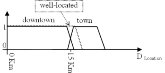
Figure 5: The user’s term well-located (dashed line) is rewritten with the terms downtown and town
For instance, in the query “find well-located homes”, the user specific term well-located is rewritten with the two fuzzy labels of the summaries down-town and down-town (Figure 5).
In this scenario, the initial Q query has been rewritten in a conservative manner so that ‘nothing is lost’. Thus, an empty set of summaries S = ∅ as an answer guarantees that there is really no result tuples to the query (i.e. , tset(Q) =∅). A non-empty set S = {z1. . . zm} denotes the possibility that
an-swer tuples exist, but nothing can be guaranteed (i.e. , tset(Q) ⊆!1≤i≤mRzi).
Of course tuples of!1≤i≤mRzi\ tset(Q) do not satisfy the initial query Q,
how-ever, they are close to the initial user’s query and consequently interesting since the user is in an exploratory analysis and tries to discover the content of the database.
In some cases, it could be more suitable to guarantee that answers exist instead of guaranteeing empty answers only. To achieve this, the initial query has to be rewritten using subsets of linguistic labels, using the usual fuzzy inclusion:
F ⊆ G iff ∀x ∈ DA, µF(x) ≤ µG(x) .
For instance, the term well-located is only mapped to downtown (Figure 5). In this second rewriting scenario, a non-empty set S = {z1. . . zm} as an answer
guarantees that all tuples covered by its summaries are really in the result of the query (i.e. ,!1≤i≤mRzi ⊆ tset(Q)) but there could be others (i.e. ,
tset(Q)-\!1≤i≤mRzi) that satisfy predicates and do not belong to S.
Note that both scenarios can be used together for the same query, as one guarantees null answers and the other guarantees non-null answers. This dual approach can be viewed as reasoning with both Possibility and Necessity (see [27]) of the query result. Moreover, these two scenarios are the boundaries of a spectrum of possible strategies: the generalized expression of the rewriting process consists in defining a threshold τ to decide whether the mapping of two fuzzy labels is correct. The user’s label d is mapped to a summary label l if and only if the similarity of d to l, denoted by σ(d, l), is greater than or equal to τ. The measure σ(d, l) evaluates the satisfiability [28] of a summary fuzzy set l to a user’s fuzzy set d. In this work, we use the following definition:
σ(d, l) = M (d∩ l)/M(l)
Assuming the usual definition of the fuzzy intersection µl∩d = min(µl, µd) and
the following fuzzy measure M:
M (l) = " #
x∈DAµl(x) if DA is finite
$
DAµl(x).dx otherwise.
Note that when τ = 0+(respectively τ = 1), we fall back into the Possibility
(respectively Necessity) scenario.
Once the query is rewritten, the ESRA algorithm, could be performed in order to provide the summarized answer. Relevance of summaries in the result depends on the query mapping and especially the satisfiability degree of the rewritten predicates. Thus, we propose in the following to sort the query results using their satisfaction to the user’s query.
6.2 Sorting the results
Consider an initial user’s query Q, expressed using her own vocabulary: “find all results which are d or d! on A
i and d!! on Aj”. The set of attributes
for which required features exist is X = {Ai, Aj} and the representation QX of
Qis:
QX = {QAi, QAj} where QAi = {d, d
!} and Q
Aj = {d
!!}
The querying process is performed using Q!, the rewritten version of Q. Each
summary z from Q! results is represented by a set of descriptors in L
Ai(z) on
each attribute Ai. For instance, LAi(z) = {l, l!}. Once we have the query and
the answers represented by linguistic descriptors, we can define a scoring func-tion based on degree of matching between the summary and query predicates, using fuzzy set operations. This choice is justified since fuzzy sets can be given a semantic in terms of degree of satisfiability. Indeed, we use σ(d, l) to com-pute the degree of matching of each query required feature (d) from QAi and
each result description (l) from LAi(z). Thus, the global degree of matching
σG(QAi, LAi(z)) between LAi(z) and QAi is a combination of all the pairwise
degrees. The simplest way to combine these degrees is by using a disjunctive aggregation that aggregates values as an OR operator, so that the result of the combination is high if some (at least one) values are high. Disjunctive combi-nation is typically performed in fuzzy set theory by T-conorm operators, whose most used instance is ’max’. Thus, we obtain:
σG(QAi, LAi(z)) = max
l∈LAi(z),d∈QAi
σ(d, l)
The function σG establishes a comparison, attribute by attribute. Thus,
we obtain as many values of comparison as there exist attributes with required features. A last aggregation step of those values is then necessary. The simplest way to do this is by using a conjunctive operator, where we require that each of the result descriptions matches the corresponding part in the query. For instance, we use the product operator to evaluate the degree of satisfiability between a given query Q and each answer z. We compute a score(Q, z) of each answer z which represents the degree to which z is relevant for the user query Q. Such a score is defined as follows:
score(Q, z) = %
Ai∈X
σG(QAi, LAi(z))
Thus, for each answer z from S (the set of Q! results returned by ESRA),
we compute its score score(Q, z); then we sort these results by their score in decreasing order; and finally return the fully ordered list Ssorted to the user.
Furthermore, when a user decides to explore a summary z! of S
sorted using the
SHOWCAT option, we sort the set of children of z! according to their scores in
decreasing order. Note that all basic needed values σ(d, l) are available because z! intent includes the intent of its children. Likewise, when a user decides to
explore a summary z! of S
sortedusing SHOWTUPLES option, each tuple t can
be sorted by score(Q, t). Indeed, if t takes value x on attribute Ai, LAi(t) = {x}
is the fuzzy set whose membership function is defined as follows:
∀y ∈ DAi, µx(y) =
"
1 if y = x; 0 otherwise.
7 Experimental Results
Evaluating and comparing the effectiveness of different approaches that address the Many answers problem in databases is challenging. Unlike Information Retrieval where there exist extensive user studies and available benchmarks (e.g. , the TREC1 collection), such infrastructures are not available today in
the context of Relational Databases. Nonetheless, in this section, we discuss the efficiency and the effectiveness of ESA, ESA+SEQ and ESRA processes based on a real database.
7.1 Data Set
Through an agreement, the CIC Banking Group provided us with an extract of statistical data used for behavioral studies of customers. The dataset is a collection of 33735 customers defined on 70 attributes (e.g. , age, income, occupation, etc.). For the results presented in this paper, we used a subset of 10 of the most relevant attributes. On each attribute, marketing experts defined between 3 and 8 linguistic labels leading to a total of 1036800 possible descriptor combinations (i.e. , 1036800 possible cells). Note that all the experiments were done on a 1.7GHz P4-based computer with 768MB memory.
7.2 Results
In this section, we validate our process (ESRA) for clustering query results with regard to performance (computational time) and usability. All experiments reported in this section were conducted on a workload composed of 150 queries with a random number of selection predicates from all attributes (i.e. , each query has between 1 and 3 required features on 1, 2, 3 or 4 attributes).
Quantitative Analysis
The CIC dataset is summarized by the SaintEtiQ summarization process as described in Section 3. The whole summarization is completed in 9min. The dataset, consisting of 33735 records, yields a summary tree with 13263 nodes, 6701 leaves, maximum depth of 16, average depth of 10.177, maximum width of 14 and an average width of 2.921. The data distribution in the summary tree reveals a 0.6% ( 6701
1036800) occupation rate.
From the analysis of theoretical complexities, we claim that ESA and ESRA algorithms are much faster than the post-clustering process ESA+SEQ. That is the main result of Figure 6 that shows the performance evolution according to the number of cells populated by query answer records. Furthermore, we plot in this figure the number of tree nodes visited (#Visited Nodes) per query (right scale) and finally the normalized ESRA time cost (tN. ESRA) to evaluate
the performance of the ESRA regardless of how query fits the pre-clustering.
tN. ESRA is computed as follows:
tN. ESRA =tESRA#Visited Nodes· #Tree Nodes.
0 500 1000 1500 2000 2500 Number Of Cells 0.0 2.0 4.0 6.0 8.0 10.0 12.0 C P U T im e ( x1 0 0 0 m se c) 0 2000 4000 6000 N u m b e r O f N o d e s ESA+SEQ #Visited Nodes ESA (Search) ESRA (ESA+Rearrange) Normalized ESRA Linear Reg. N. ESRA
y=x.ln(x)
y=x
Figure 6: Time cost comparison
As one can observe, the ESA+SEQ approach is quasi-linear (O(L·log(L))) in number of cells L whereas ESA, ESRA and N. ESRA processes are linear (O(L)). Besides, the time cost incurred by rearranging query results (i.e. , tESRA−tESA)
is insignificant compared to search cost (i.e. , tESA). Thus, the ESRA algorithm
is able to drastically reduce time cost of clustering query results.
Qualitative Analysis
Due to the difficulty of conducting a large-scale real-life user study, we discuss the effectiveness of our clustering process of query answers (ESRA) based on structural properties of results provided to the end-user. It is worth noticing that the end-user benefit is proportional to the number of items (clusters or tuples) the user needs to examine at any time as well as dissimilarity between these items.
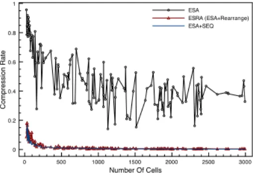
We define the ‘Compression Rate’ (CR) as the ratio of the number of clusters returned as a starting point for an online exploration over the total number of cells covered by such clusters. As expected, Figure 7 shows that CR values of ESRA and ESA+SEQ approaches are quite similar and much smaller than that of ESA process. Note that CR = 1 means no compression at all, whereas smaller values represent higher compression. As one can observe, size reduction is clearly achieved by the ESRA process.
0 500 1000 1500 2000 2500 3000 Number Of Cells 0 0.2 0.4 0.6 0.8 1 Compression Rate ESA ESRA (ESA+Rearrange) ESA+SEQ
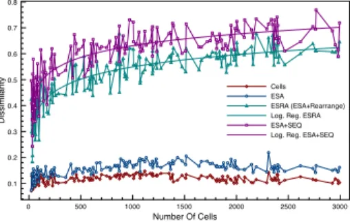
We could also see that the dissimilarity (Figure 8) of the first partitioning that ESRA process presents to the end-user is greater than that of ESA approach and is in the same order of magnitude than that provided by the ESA+SEQ approach. It means that ESRA process significantly improves discrimination between items when compared against ESA approach and is as effective as the post-clustering approach ESA+SEQ. Furthermore, the dissimilarity of the ESA result is quite similar to that of the most specialized partitioning (set of cells). Thus the rearranging process is highly required to provide the end-user with well-founded clusters. 0 500 1000 1500 2000 2500 3000 Number Of Cells 0.1 0.2 0.3 0.4 0.5 0.6 0.7 0.8 Dissimilarity Cells ESA ESRA (ESA+Rearrange) Log. Reg. ESRA ESA+SEQ Log. Reg. ESA+SEQ
Figure 8: Dissimilarity comparison
In the following, suppose a user considers that a summary z seems relevant (exactly or partially) to her. She explores z using either SHOWTUPLES or SHOWCAT option until she reaches every relevant tuple. Thus, the number of hops NoH (i.e. , the number of SHOWTUPLES/SHOWCAT operations) required to reach relevant data ranges from 1 up to dz + 1, where dz is the
height of the tree rooted by z (i.e. , subtree Hz). The best case occurs when
z exactly meets user’s need whereas the worst case occurs when the relevant information is reached by following a path of maximal length in Hz. Note
that these two scenarios are on opposite extremes of the spectrum of possible situations: the generalized case is that the user’s requirement is exactly satisfied by a node (i.e. , not necessarily the root or a leaf node) of Hz. In this experiment,
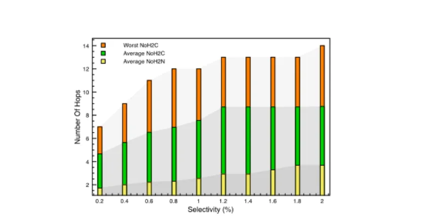
one considers a user query q with selectivity of η percent, i.e. , the ratio of the number of cells covered by q results over the number of cells of the pre-computed tree. We look for all the possible summaries (subtrees) in the pre-computed tree that can be returned as the result of q and, for each one, we compute its maximum depth, its average depth and the average length of all paths emanating from that node (summary). Then, we pick out the highest (maximum) value observed for each of these measures. The three values obtained, for each value of η (η =∈ {0.2, 0.4 . . .2}), evaluate respectively: (1) the worst number of hops required to reach the deepest leaf (cell) node (Worst NoH2C) containing relevant data; (2) the average number of hops needed to reach any leaf node (Average NoH2C) containing relevant data (i.e. not necessarily the deepest one); (3) the average number of hops required to reach any node (Average NoH2N) containing relevant data (i.e. , not necessarily a leaf node).
Figure 9 shows that the Worst NoH2C and the Average NoH2C are relatively high, but bounded respectively by the maximum (16) and the average (10.177) depth of the pre-computed tree. It is worth noticing that, in real life situation,
0.2 0.4 0.6 0.8 1 1.2 1.4 1.6 1.8 2 Selectivity (%) 2 4 6 8 10 12 14 Number Of Hops Worst NoH2C Average NoH2C Average NoH2N
Figure 9: The number of SHOWTUPLES/SHOWCAT operations
the user finds out that her need has successfully served by an inner node of the tree rooted by z. Thus, the Average NoH2N is more adapted to evaluate the effectiveness of our approach (ESRA). As one can observe, the Average NoH2N is quite small (e.g. , 3.68 hops to locate relevant information within a collection of 674 records).
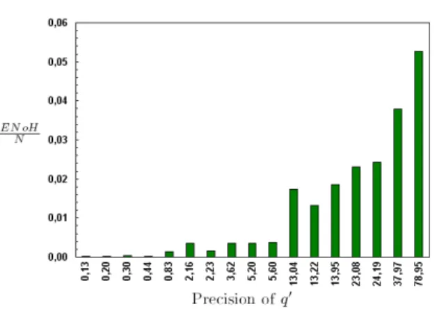
Finally, we aim to compare the number of results the user has to examine until she reaches relevant data when answers are rearranged using ESRA or not. To this end, we pick randomly one summary z from the lower part of the pre-computed tree (e.g. , z covers 30 cells) and generate the query q that returns z. Assume that z exactly fits user’s need, i.e. , the user is interested in all tuples (Rz) that mach q (P recision = Recall = 1). Further, assume that
such user submits a broad query q! instead of q, i.e. , q! is a relaxation of q
and consequently matches a superset of Rz (P recision < 1 and Recall = 1).
In this experiment, the additional selection predicates in the query q are used to model user’s actions to get exactly what she wants when browsing through q! results. Note that when no processing has been performed on q! results,
the user has to examine N cells in order to get all relevant tuples (Rz), where
N is the number of cells that satisfy q!. However, when q! is processed using
our ESRA algorithm, the user has to examine only ENoH clusters and then performs one SHOWTUPLES operation; ENoH is the effective number of hops (or SHOWCAT operations) required to reach z. This is due to the fact that our ESRA algorithm provides a clustering schema of q! results where all cells that fit
user’s need are grouped into a single cluster (i.e. z) which does not overlap with irrelevant ones, if we except overlapping of borders of fuzzy cells. Figure 10 shows the evolution of EN oH
N according to the precision of q!. The precision
of q! is the ratio of the number of relevant cells (30) over the number of cells
that match the broad query q! (N). As one can observe,EN oH
N is much smaller
than 1. For instance, EN oH
N is equal to 0.0013 ( 5
3603) for a query precision of
0.0083 ( 30
3603). It means that only 5 hops are required to locate the summary
z within a clustering schema of q! results that covers 3603 cells. Thus, ESRA
is able to drastically reduce the ‘Information Overhead’ that user experiences when submitting a broad query.
Those experimental results validate the claim of this work that is to say the ESRA algorithm is very efficient and achieves high quality results and conse-quently makes the exploration process more effective.
Figure 10: Effectiveness of ESRA regarding the precision of query’s results
8 Conclusion
Interactive and exploratory data retrieval are more and more suitable to database systems. Indeed, regular ‘blind’ queries often retrieve too many answers. Users then need to spend time sifting and sorting through this information to find relevant data. In this communication, we propose an efficient algorithm coined Explore-Select-Rearrange Algorithm that quickly provide the user with concise and well-formed clustering schema of a query results. Indeed, clusters of a user query results are targeted elements of the hierarchical grid-based clustering of the whole data set (computed offline) and every subtree rooted by each answer offers a guided tour of the data subset to the user. Experimental results show that our process is efficient, provides well-formed clusters (their number is small and they are well separated) and then is very helpful in a situation when a user has not a specific retrieval goal and is interested in browsing through a set of items to explore what choices are available.
Note that Explore-Select-Rearrange Algorithm, in its current state, returns results using linguistic variables of summaries even if user expresses her query using a free vocabulary. A future work is then to perform results rewriting.
References
[1] J. Minker, An Overview of Cooperative Answering in Databases, FQAS98, 282-285, 1998.
[2] H. Ferhatosmanoglu et al, High dimensional nearest neighbor searching, Inf. Syst. 0306-4379, 2006.
[3] L. Wu et al, FALCON: Feedback Adaptive Loop for Content-Based Re-trieval, VLDB00, 297-306, 2000.
[4] S. D. MacArthur et al, Interactive content-based image retrieval using rel-evance feedback, Comput. Vis. Image Underst. 55–75, 2002.
[5] S. Agrawal et al, Automated Ranking of Database Query Results, CIDR03, 2003.
[6] C. Surajit et al, Probabilistic Ranking of Database Query Results, VLDB04, 888-899, 2004.
[7] I. Ilyas et al, A survey of top-k query processing techniques in relational database systems, ACM Computing Surveys, 2008.
[8] M. A. Hearst, J. O. Pedersen, Reexamining the Cluster Hypothesis: Scat-ter/Gather on Retrieval Results, SIGIR96, 76-84, 1996.
[9] H. J. Zeng et al, Learning to cluster web search results, SIGIR04, 210-217, 2004.
[10] D. Cheng et al, A divide-and-merge methodology for clustering, SIGMOD-SIGACT-SIGART 05, 196-205, 2005.
[11] P. Ferragina et al, A personalized search engine based on web-snippet hier-archical clustering, WWW05, 801-810, 2005.
[12] K. Chakrabarti et al, Automatic categorization of query results, SIGMOD04 ,755-766, 2004.
[13] B. Bamba et al, OSQR: overlapping clustering of query results, CIKM05, 239-240, 2005.
[14] C. Li et al, Supporting ranking and clustering as generalized order-by and group-by, SIGMOD07 ,127-138, 2007.
[15] R. Saint-Paul et al, General purpose database summarization, VLDB05,733-744, 2005.
[16] L. A. Zadeh, Information and Control, Fuzzy Sets, 8:338-353, 1956. [17] L. A. Zadeh, Concept of a linguistic variable and its application to
approx-imate reasoning, Information and Syst˙, 1:119-249, 1975.
[18] L. A. Zadeh, Fuzzy sets as a basis for a theory of possibility, Fuzzy Sets and Syst˙, 100:9-34, 1999.
[19] K. Thompson et al, Concept Formation in Structured Domains, Concept formation: Knowledge and experience in unsupervised learning, 127-161, 1991.
[20] E. Rosch et al, Family ressemblances: studies in the internal structure of categories, Cognitive Psychology, 7:573-605, 1975.
[21] A. Tversky, Features of similarity, Psycol ˙Rev˙, 84(4):327-352, 1977. [22] M. Halkidi et al, Clustering validation, Jour. of Intelligent Info. Syst˙,
17:107-145, 2001.
[23] A. Guttman, R-trees: a dynamic index structure for spatial searching, SIGMOD84, 47-57, 1984.
[24] D. Papadias et al, Efficient OLAP Operations in Spatial Data Warehouses, SSTD01, 443-459, 2001.
[25] Y. Tao et al, Range Aggregate Processing in Spatial Databases, TKDE04, 16:1555-1570, 2004.
[26] R. R. Yager, Connectives and quantifiers in fuzzy sets, Fuzzy Sets and Syst˙, 40(1):39-75, 1991.
[27] D. Dubois et al, A new perspective on reasoning with fuzzy rules, In-ter ˙Jour˙of Intelligent Syst˙, 18(5):541-563, 2003.
[28] B. Bouchon-Meunier et al, Towards general measures of comparison of objects, Fuzzy Sets Syst˙, 84(2):143-153, 1996.
Contents
1 Introduction 3
2 Related work 4
3 Overview of the SaintEtiQ System 5
3.1 A Two-Step Process . . . 5
3.1.1 Mapping Service . . . 5
3.1.2 Summarization Service . . . 6
3.2 Features of Summaries . . . 7
3.3 Discussion about SaintEtiQ . . . 8
4 Querying the SaintEtiQ Summaries 8 4.1 Expression and Evaluation of a Query . . . 10
4.2 Search algorithm . . . 10
4.3 Multi-Scale Summarized Answers . . . 12
5 Rearranging query results 14 6 Discussion about Extension to any Fuzzy Predicate 16 6.1 Query rewriting . . . 17
6.2 Sorting the results . . . 19
7 Experimental Results 20 7.1 Data Set . . . 20
7.2 Results . . . 20
Centre de recherche INRIA Grenoble – Rhône-Alpes : 655, avenue de l’Europe - 38334 Montbonnot Saint-Ismier Centre de recherche INRIA Lille – Nord Europe : Parc Scientifique de la Haute Borne - 40, avenue Halley - 59650 Villeneuve d’Ascq
Centre de recherche INRIA Nancy – Grand Est : LORIA, Technopôle de Nancy-Brabois - Campus scientifique 615, rue du Jardin Botanique - BP 101 - 54602 Villers-lès-Nancy Cedex
Centre de recherche INRIA Paris – Rocquencourt : Domaine de Voluceau - Rocquencourt - BP 105 - 78153 Le Chesnay Cedex Centre de recherche INRIA Saclay – Île-de-France : Parc Orsay Université - ZAC des Vignes : 4, rue Jacques Monod - 91893 Orsay Cedex
Centre de recherche INRIA Sophia Antipolis – Méditerranée : 2004, route des Lucioles - BP 93 - 06902 Sophia Antipolis Cedex
Éditeur
INRIA - Domaine de Voluceau - Rocquencourt, BP 105 - 78153 Le Chesnay Cedex (France)
http://www.inria.fr ISSN 0249-6399