HAL Id: halshs-00552242
https://halshs.archives-ouvertes.fr/halshs-00552242
Preprint submitted on 5 Jan 2011
HAL is a multi-disciplinary open access archive for the deposit and dissemination of sci-entific research documents, whether they are pub-lished or not. The documents may come from teaching and research institutions in France or abroad, or from public or private research centers.
L’archive ouverte pluridisciplinaire HAL, est destinée au dépôt et à la diffusion de documents scientifiques de niveau recherche, publiés ou non, émanant des établissements d’enseignement et de recherche français ou étrangers, des laboratoires publics ou privés.
Yardstick competition in a Federation: Theory and
Evidence from China
Emilie Caldeira
To cite this version:
Emilie Caldeira. Yardstick competition in a Federation: Theory and Evidence from China. 2011. �halshs-00552242�
CERDI, Etudes et Documents, E 2010.18
Document de travail de la série
Etudes et Documents
E 2010.18
Yardstick competition in a Federation: Theory and
Evidence from China
Emilie Caldeira*
May 2010
* CERDI-CNRS, Université d'Auvergne, Economics Dept
Mail address: 65 boulevard François Mitterrand, 63000 Clermont-Ferrand, France Email: emiliecaldeira@gmail.com
Yardstick competition in a Federation: Theory and
Evidence from China.
May 2010
Abstract
While some scholars argue that …scal decentralization gave Chinese local o¢ cials strong incentives to promote local economic growth, traditional …scal federalism theories are not directly relevant to explain such an e¤ect in the particular context of China. In this paper, we explain the existence of interjurisdictional competition among Chinese local o¢ cials using a model of yardstick competition "from the top", in which the central government (and not local voters) creates a competition among local o¢ cials by rewarding or punishing them on the basis of relative economic performance. Our model predicts that, in this context, local governments are forced to care about what other incumbents are doing and that public spending settings are strategic complements. Then, by estimating a spatial lag dynamic model for a panel data of 29 Chinese provinces from 1980 to 2004, we provide empirical evidence of the existence of such public spending interactions. We propose a rigorous empirical framework which takes into account heterogeneity, simultaneity and endogeneity problems and spatial error dependence. The results are encouraging to the view that there are some strategic interactions among Chinese provinces, resulting from a yardstick competition created by the central government.
JEL Classi…cation: D72, H2, H7
Keywords: Decentralization, China, public spending interactions, yardstick competition, spatial panel data.
Emilie Caldeira,z
z: CERDI-CNRS, Université d’Auvergne, Economics Dept
Mail address: 65 boulevard François Mitterrand, 63000 Clermont-Ferrand, France Email: emiliecaldeira@gmail.com
1
Introduction
China’s remarkable growth in the 1980s and 1990s coincided with the …scal decentraliza-tion. Some scholars argue that the latter gave Chinese local o¢ cials strong incentives to promote local economic growth, creating a basis for nationwide high economic performance (Qian and Weingast (1997), Zhuravskaya (2000), Qian (2003) and Jin, Qian, and Weingast (2005)). Though, traditional …scal federalism theories are not directly relevant to explain such an e¤ect in the context of China. In particular, the existence of a yardstick competition among local governments, a traditional argument in favor of decentralization in democratic countries, is not relevant a priori in China where the local o¢ cials are not elected by citizens. Blanchard and Shleifer (2000) have previously argued that in China, the central government is in a strong position both to reward or to punish local administrations, insuring political accountability of local o¢ cials. We provide here evidence of a yardstick competition "from the top", in which the principal is the central government and not the local population. Thus, we propose an explanation of the existence of interjurisdictional competition among Chinese local governments.
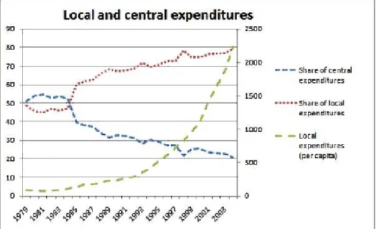
Fiscal decentralization has been a critical component of economic reform in China. In-deed, substantial e¤orts have been made to decentralize its formerly highly centralized …scal management system to provincial governments. The latter have been given considerable latitude in shaping local policies and managing …scal resources: more than 70 percent of the entire public expenditure was made at the sub-national levels in 2004 (see Figure 2 in Appendix A.2.1).1 However, as noted before, "Chinese style decentralization" is actually conceptually di¤erent from decentralization in many other countries. Indeed, China’s cur-rent …scal system is largely decentralized while its governance structure is rather centralized with strong top-down mandates and a homogenous governance structure. For Maskin, Qian, and Xu (1997), it can be described as a multidivisional-form hierarchy structure. The
cen-1
Provincial levels are …rst-level local state administrative organs in China. In this paper, we will focus on this jurisdiction level. The country is divided into three levels: the province, the county, and the township. However, two more levels have been inserted in actual implementation: the prefecture, under the provincial level; and the village, under the township level. By conventional measure, there are …ve tiers in China …scal system: the central government, 33 province-level regions, 333 prefecture-level regions, 2,862 county-level regions and 44,741 township-level regions. The 33 provincial-level administrative units include 22 provinces, …ve autonomous regions, four municipalities and two special administrative regions.
tral government exerts great in‡uence on the local administrations’actions.2 Moreover, the power of provincial governments is not based on a system of electoral representation: the governors are appointed by the central government in Beijing. Lastly, the population mobil-ity between local jurisdictions still limited in spite of the relaxations of the Hukou system. In this context, traditional disciplining devices such as local election and exit option are far from perfect. Indeed, in traditional …scal federalism theory, decentralization is supposed to increase the e¢ ciency of public spending by inducing interjurisdictional competition among political powers, through a "vote with feet" or a yardstick competition created by local voters. A priori, these theories are not relevant in the context of China.3
However, following Blanchard and Shleifer (2000), we argue that vertical control can en-sure local accountability of local o¢ cials and induces some interjurisdictional competition. Indeed, Tsui (2005) describes how Chinese provincial leaders operate within a well-de…ned career structure inside the political hierarchy. They undergo detailed performance reviews by their superiors, and are rewarded or penalized based on their success in achieving speci…c targets. Promotions, demotions, and job related bene…ts all depend on such reviews, which have become increasingly formal.4 Maskin, Qian, and Xu (1997) actually show that provin-cial o¢ provin-cials are more often promoted to the Party’s Central Committee if their province’s relative growth rate increases. Similarly, Li and Zhou (2005) examine careers of top o¢ cials in 28 provinces form 1979 to 1995 and …nd that promotions are signi…cantly more likely in provinces with higher growth. This con…rms anecdotal evidence showing that Chinese cadres are evaluated in accordance with their economic performance. So, career concerns may create strong incentives to improve economic performance like in democratic countries. Local governors may consider the risk of damaging their career since the probability of their reappointment depends on how well they perform in ful…lling their mandates from above.5
2
China’s intergovernmental relations are a hierarchical system of bureaucratic control where provincial governments must accept the uni…ed leadership of the State Council which has the power to decide on the division of responsibilities and to annul inappropriate decisions and orders of provincial governments. A representative of the Communist Party of China is appointed by their supervisors and acts as the policy maker. The Party Secretary is always in precedence above the leader of the People’s Government.
3
We can note that there are elections at village level. In this context, using a sample of rural Chinese villages, Brandt and Turner (2006) …nd that even very poorly conducted elections can have large incentive e¤ects: elections provide a disincentive for rent seeking.
4 Under Mao, promotion in part depended on ideological conformity but as reformers came to dominate in
the 1980s, targets increasingly focused on economics. As of the mid-1990s, the system for evaluating provincial leaders assigned 60 out of 100 points to targets related to economic performance (Zhang (2006)).
5
Under this structure, the central government can make comparisons between local jurisdic-tions to appraise local government’s relative performance and create a yardstick competition among local o¢ cials by rewarding or punishing them on the basis of economic performance. The idea that performance of local governments can be evaluated by cross-jurisdictional comparisons was previously proposed by Salmon (1987) and formally developed by Besley and Case (1995b). Here, we modify the model of the latter to apply yardstick competition to China. This competition is "from the top" since the principal is the central government, and not the local "voting" populations. A second modi…cation with respect to Besley and Case (1995b) is to introduce the possibility of being promoted. By this way, we propose a possible explanation of the existence of interjurisdictional competition among Chinese local governments despite the absence of electoral accountability.
This paper develops a model of public spending setting in a multijurisdictional world with asymmetric information, where the central government makes comparisons between local jurisdictions to overcome political agency problems. Finally, as in the traditional yardstick competition model, information spillovers from other jurisdictions a¤ect the delivery of public services in a jurisdiction. This forces local o¢ cials into a yardstick competition in which they care about what other local o¢ cials are doing. Thus, the theoretical model predicts that, when the central government uses neighboring performance to judge a governor, the latter is encouraged to follow neighboring …scal choices in order not to be signaled as bad local government and to be reappointed. So, in presence of yardstick competition "from the top", we should observe strategic interactions among local decision-makers and public choices should be strategic complements. Strategic complements refer to the de…nition by Bulow, Geanakoplos, and Klemperer (1985) of the nature of competition. The latter de…ne public spending as strategic complements when the marginal utility of public spending in jurisdiction i is increasing in the level of local public spending in the other jurisdictions.
Then, this paper proposes a rigorous empirical framework which takes into account het-erogeneity, simultaneity and endogeneity problems and spatial error dependence to test the-oretical model’s predictions. Our empirical analysis actually provides evidence of the ex-istence of interjurisdictional competition among local governments embedded in a vertical
bureaucratic control system. To our knowledge, this study is the …rst attempt to test public spending interactions in China. Indeed, most of the empirical literature focuses on strategic interactions with respect to taxes in developed countries. Little attention has been paid to the public expenditures side6 a fortiori in developing or emerging countries.7
The paper is structured as followed: Section 2 develops a theoretical model of yardstick competition "from the top"; Section 3 estimates a spatial lag model for a panel data of 29 Chinese provinces from 1980 to 2004 to test the existence of public spending interactions, resulting from a yardstick competition "from the top". Section 4 concludes.
2
Theoretical framework: decentralization and yardstick
com-petition "from the top"
As Besley and Case (1995a) showed, economic considerations alone cannot characterize eco-nomic policy choices at local level. Political mechanisms and electoral accountability seem to a¤ect economic policy choices. The idea that residents consider neighboring jurisdictions as a yardstick to compare the performance of their local government and judge whether they waste resources and deserve to remain in o¢ ce was initially proposed by Salmon (1987). He insights that much of the thinking behind the theory of labor tournaments of Lazear and Rosen (1981), Holmstrom (1982) or Shleifer (1985) could be applied to interjurisdictional competition. Besley and Case (1995b) introduced yardstick competition between jurisdic-tions as a discipline device for rent-seeking politicians in the context of a developed and democratic country.
This paper modi…es the traditional approach of Besley and Case (1995b) by consider-ing a model of yardstick competition "from the top" in which the principal is the central government and not local populations. Moreover, we focus on the public spending side and
6
We can mention the works of Redoano (2007) or Foucault, Madies, and Paty (2008). They …nd that some interactions take place among neighboring jurisdictions with respect to expenditures for respectively EU countries and French municipalities.
7 Akin, Hutchinson, and Strumpf (2005) analyze the decentralization of health care competences in Uganda
and provide evidence for the hypothesis that spillover e¤ects cause spending on public goods in one district to reduce spending in neighboring districts. Arze, Martinez-Vasquez, and Puwanti (2008) focus on local discretionary expenditures in Indonesia and highlight strategic complementarity of local public spending. Caldeira, Foucault and Rota-Graziosi (2009) have also found strategic complementarity among local public spending among Beninese municipalities.
introduce the possibility for local governments to be promoted.8
2.1 The model
Following Besley and Case (1995b), we consider a principal/agent model.
1. The agents are local o¢ cials. They are assumed to know more about the short term economic shocks at local level than do the central government.
2. The principal is here, the central government. He is assumed to use performance cues of other local o¢ cials as a benchmark to appraise whether agents waste resources and deserve to remain in o¢ ce.
3. The main incentive mechanisms used to discipline governors are reappointment and promotion (instead of elections). The central government decides whether or not to reappoint an agent and can promote an agent who is non-revealed as bad.9
We consider a jurisdiction whose local government provides public services of a given quality (Gi) …nanced by taxes (t). The …nal level of …scal revenue is t k, with k stochastic
and observed only by the local government. As in Besley and Case (1995b), the product
k can take one of three values, high (H), medium (M ) or low (L) with probabilities qH;
qM and qL. So, we have three values of taxes revenue, assumed to be evenly spaced with
di¤erence (as Besley and Case (1995b) do).
The local governments are potentially of two kinds: "good" (g) or "bad" (b).10 Agent’s strategies are denoted:
G( k; j); (1)
8 We generally simplify matters by assuming that bureaucrats may either be re-appointed or dismissed.
In reality, other rewards and punishments may be meted out to them in China. Indeed, upper levels of governments have the power to appoint and dismiss but also to promote subordinate cadres. The promotion opportunities that lie ahead for provincial secretaries include membership of the State Council, the vice premiership, the premiership and membership of the Politburo or the Politburo Standing Committee.
9 Theoretically, it is equivalent to consider the reappointment and the promotion for a non revealed bad
o¢ cial or the "retirement" and the demotion for the revealed bad o¢ cial.
with k (H; M ; L) and j (g; b). Good local governors do not rent-seeking or waste resources while bad ones do it. The latter can subtract or 2 as rent or waste. Formally, we have:
G( k; g) = t k; (2)
and
G( k; b) = t k ri;
with ri, the rent which may take two values: and 2 .
As in Besley and Case (1995b), we consider two time periods. The discount factor is and satis…es 1 > > 1=2. The central government observes public spending decisions and updates its beliefs that the agent is good. Then, it chooses whether or not to reappoint him since it wants to maximize public spending for a given level of taxes. The central government strategy is denoted by
(Gi) [0; 1]; (3)
which corresponds to the probability that he reappoints an local governor who sets a public spending level Gi:
Bad local o¢ cial chooses public spending to maximize his discount utility which positively depends on the rent in period 1 and on expected rent and promotion in period 2:
E [V (Gij k)] = ri+ (Gi) (2 + 'p); (4)
A bad o¢ cial who is reappointed sets no period 2 discipline and takes a rent equal to 2 . Moreover, a non revealed bad agent can be promoted in period 2 with an exogenous probability of ', which gives him an utility of p:11 So, he arbitrates between the rent in period 1 and the expected utility in period 2 knowing that his probability of being reappointed depends on the level of public spending provided in period 1.12
1 1
A promotion means a move by a provincial leader up to his position.
1 2 Note that, by assumption, there is no sanction, i.e, local government is not bound to give back what he
2.2 Perfect information: the centralized …scal system
As a benchmark, we …rst consider the case in which the …scal system is centralized and information is perfect.
All tax revenues are collected by the central government at local level and transferred back to local governments according to a plan of spending made by the center. Formally, we have:
Gi= Ti ri; (5)
with Gi, the level of public spending, Ti; the …scal revenue transferred by the central
gov-ernment and ri, the rent.
In this case, a local government who sets a level of public spending smaller than the …scal revenue transferred by the central government will be automatically signaled as bad local government and will not be reappointed. Hence, if the expected utility of being promoted is high enough, bad o¢ cial will always take no rent in period 1 to be reappointed in period 2, with or without yardstick competition. Indeed, since there is no information to reveal, yardstick competition is useless and has no e¤ect on local o¢ cial public spending choices which are independent on what other agents are doing.
Proposition 1 Under perfect information, the equilibrium is: (i) All types of agents 13 set:
Gi = Ti:14
(ii) Central government sets:
(Ti ) = (Ti 2 ) = 0 and (Ti) = 1:
Proof. See Appendix A.1.1
Corollary 1 Under perfect information:
(i) The yardstick competition "from the top" has no impact on local governments’ spending
1 3
For bad local government, this is the case if 'p > (2 2 )= . We consider that it is the case for the rest of the paper.
decisions;
(ii) Public spending choices are independent from each other: there is no horizontal strategic interaction;
In a centralized …scal system, the central government knows the level of tax revenue. He does not need to make comparisons between local jurisdictions to determinate local o¢ cial’s type. Yardstick competition is useless and public spending choices are independent from each other. So, when the …scal system is centralized, we should not observe any horizontal strategic interactions among local governments.
2.3 Asymmetric information: the decentralized …scal system
We now consider the decentralized case with asymmetric information between the local o¢ -cials and the central government.
First, as in Besley and Case (1995b), we consider that nature selects the type of the local government which will be "good" with probability and "bad" with probability (1 ): Nature determines also the product which will be high with probability qH; medium with
probability qM and low with probability qL.15
Second, we deduce …ve possible public spending levels, fG1; G2; G3; G4; G5g with G1 >
G2 > G3 > G4 > G5 where:
Good governor provides services consistent with the true level of tax revenue in the two periods:
G( H; g) = t H = G1 and G( M; g) = t M = G2 and G( L; g) = t L= G3:
Bad governor can choose to take no rent, a rent of or a rent of 2 . According to the products, the level of public spending can be:
–when the product is high:
G( H; b) = t: H = G1 or t H = t M = G2 or t H 2 = t: L= G3; 1 5 To simplify, we consider q
–when the product is medium:
G( M; b) = t M = G2 or t M = t: L= G3 or t M 2 = G4;
–when the product is low: G( L; b) = t L = G3 or t L = t M 2 = G4 or
t L 2 = G5:
The following table sums up the possible levels of public spending:
Agent n Product High Medium Low
Good G1 G2 G3
Bad r= 0 r= r= 2 r= 0 r= r= 2 r= 0 r= r= 2
G1 G2 G3 G2 G3 G4 G3 G4 G5
Third, the central government observes public spending and choices whether or not to reappoint the local government to maximize expected public spending in period 2.
See the extensive-form game in Appendix A.1.2.
2.3.1 Perfect Bayesian equilibrium without Yardstick Competition
We consider …rst, one jurisdiction and we …nd perfect Bayesian equilibrium of the public spending game.
Our model predicts that without yardstick competition, the bad o¢ cial takes a maximal rent when the product is low ( L) or medium ( M). Indeed, in those cases, the central
government will always believe that a local government who sets G4 or G5 is bad but it also
does not …nd it worthwhile to reappoint any local governor who sets G2 or G3. So, providing
higher level of public spending (G2 or G3) gets less rent with no gain in the probability of
being reappointed. Hence, bad local o¢ cial is not encouraged to reduce his rent when the product is low or medium.
On the contrary, when the product is high ( H), the central government is willing to
reappoint a local government who sets G1. Hence, with a high enough value of 'p, bad
Proposition 2 Without yardstick competition, the equilibrium is: (i) Good local governor sets:
8 > > > > < > > > > : G( H; g) = t H = G1; G( M; g) = t M = G2; G( L; g) = t L= G3:
(ii) Bad local governor sets:16 8 > > > > < > > > > : G( H; b) = t H = G1; G( M; b) = t M 2 = G4; G( L; b) = t L 2 = G5:17
(iii) Central government sets: 8 > < > : (G1) = 1; (G2) = (G3) = (G4) = (G5) = 0:18
Proof. See Appendix A.1.3
In a decentralized …scal system with asymmetric information between the central gov-ernment and local govgov-ernments, the latter are not encouraged to reduce their rent. This is the case because, when the conjuncture is bad or medium, they are not able to convince individually the central government that they are good.
2.3.2 Perfect Bayesian equilibrium with Yardstick Competition
We now consider two jurisdictions with identical environments and shocks in which appointed o¢ cials may be of di¤erent types. As Besley and Case (1995b), we consider that local o¢ cials know each other types.19 We analyze the e¤ect of the central government information about
1 6 As we said before, we consider that 'p > (2 2 )= . But note that, if 'p < (2 2 )= , bad
incumbent sets: G( H; b) = t H 2 = G3 ; G( M; b) = t M 2 = G4 ; G( L; b) = t L 2 = G5
1 9
In other words, we suppose that neighboring local governments know more about each other than the central government do. The full information is maybe a bit strong.
public spending in both jurisdictions. We have two cases to consider.20
Both local governments are bad First, we consider the case where both agents are bad. The equilibrium is a perfect Bayesian equilibrium for the two agents. The full characterization of the equilibrium is given at the Appendix A.1.4.
Now, we show that both local governors choosing the same strategy gives the central government more con…dence that a local government is good.
In particular, the probability that a local government is good if we observe G3 in both
jurisdiction is, now, higher than if > 0:7: In this case, the central government is willing to reappoint a local government who sets G3: So, both agents decide to reduce their rent
when the product is low ( L) to be reappointed. Hence, since we have (G3) = 1 and
(G4) = (G5) = 0, bad governments play
G( L; b) = t L= G3;
and take no rent in period 1.21
Under this condition, the probability that a local government is good if we observe G2
in both jurisdictions is also higher than : So, the central government …nds it worthwhile to reappoint a local o¢ cial who sets G2. But since playing G2 when the product is medium
( M) gets less rent with no gain in the probability of staying in o¢ ce than playing G3, bad
agents decide to reduce their rent only up to G3 and play:
G( M; b) = t M = G3:
Lastly, when the product is high ( H), since (G1) = (G2) = (G3) = 1, providing a higher
level of public spending gets less rent with no gain in the probability of being reappointed. Bad local governor can now play:
G( H; b) = t M 2 = G3; 2 0
Besley and Case (1995b) also consider the case in which both local o¢ cials are good but this case in trivial.
Proposition 3 With yardstick competition "from the top", if both local governments are bad, the equilibrium is:
(i) Bad local governments set: 8 > > > > < > > > > : G( H; g) = t M 2 = G3; G( M; g) = t M = G3; G( L; g) = t L= G3:22
(ii) Central government sets: 8 > < > : (G1) = (G2) = (G3) = 1; (G4) = (G5) = 0:
Proof. See Appendix A.1.4
In presence of yardstick competition, local governors are able to make the central gov-ernment believe that both are good, by reducing together their rent. Indeed, choosing the same strategy gives the central government more con…dence that both are good. So, both local governments are, now, encouraged to reduce their rent when the conjuncture is bad or medium so that they will be reappointed.
One local government is good and the other is bad Second, we consider the case where one government is good and the other is bad. The full characterization of the equilib-rium is given at the Appendix A.1.5.
In this case, the bad local governor will be found out by setting public spending above its neighbor. Now, playing G3 when the product is high or medium results in being unseat:
(G3) = 0 when H or M: So, the bad o¢ cials will reduce their rent and act as good
governments. Indeed, whatever the product level, local o¢ cial prefers to take no rent in period 1 to be reappointed.
Proposition 4 With yardstick competition "from the top", if one government is good and the other is bad, the equilibrium is:
(i) Bad local governor and good local governor set: 8 > > > > < > > > > : G( H; g) = t H = G1; G( M; g) = t M = G2; G( L; g) = t L= G3:23
(ii) Central government sets: 8 > < > : (G1) = (G2) = (G3) = 1;24 (G4) = (G5) = 0:
Proof. See Appendix A.1.5.
In presence of yardstick competition, when a bad local government is compared with a good one, the bad local governor chooses the same strategy as the good one in order not to be found out.
Yardstick Competition "from the top" e¤ect When the central government makes comparisons between local jurisdictions, this forces local o¢ cials to care about what other lo-cal governments are doing, creating horizontal strategic interactions which are complements.
Corollary 2 Under our assumptions,
(i) The yardstick competition "from the top" involves horizontal strategic interactions among neighboring jurisdictions;
(ii) Under yardstick competition, public spending are strategic complements.
Local governor public spending behavior is a¤ected by the central government looking at neighboring jurisdictions. Hence, the yardstick competition created by the central govern-ment to overcome political agency problems implies horizontal strategic interactions among local o¢ cials.
Moreover, in presence of yardstick competition, public spending settings appear to be strategic complements. We have studied two cases. First, when both local o¢ cials are bad, choosing the same strategy gives the central government more con…dence that governors are good so that both bad local o¢ cials decide, as soon as possible, to reduce together their rent
so that they will be reappointed. Second, good local government in‡icts an externality on the bad one, conducing them to act as good governments to be reappointed. Finally, if a bad o¢ cial has low performance relative to its neighbor, the central government interprets this as evidence that the o¢ cial is bad and unseats him at the next appointment. So, an increase in the level of public goods in neighboring province forces i’s local government to rise its own spending if he wants to be reappointed, conducing to strategic complementary of public spending.
These results are usual in yardstick competition model. In their model of yardstick competition in which jurisdictions face the alternative to choose between an old and a new policy, Rincke (2005) also concludes that "An equilibrium with yardstick competition is shown to exist where bad governments having a good government in their neighborhood choose the new policy more often compared to an equilibrium without relative performance evaluation." Our results are also similar to those of Besley and Case (1995b). However, while Besley and Case (1995b) focus on the e¤ect of relative performance on the probability of being reelected, we focus on the e¤ect of yardstick competition on the existence of strategic interactions among local governments and their nature. Indeed, according to Canegrati (2006), we distinguish two e¤ects of the yardstick competition: a selection e¤ects, which separates good governments from bad governments and a discipline e¤ect, which forces bad governments to act as if they were good. We focus on the second one and we show how local governments are less corrupt or more e¢ cient because of more intense interjurisdictional yardstick competition.
2.3.3 Comparison on the equilibrium public spending
We can note that there is no common agreement among researchers about the ability of the yardstick competition to reach citizens’welfare. Some economists who believe that govern-ment is benevolent are prone to see inter-governgovern-mental competition as a source of negative externalities which lower welfare. On the contrary, the public choice perspective which assumes the existence of Leviathan governments sees yardstick competition as potentially bene…cial for welfare (Besley and Smart (2002)).25 Brülhart and Jametti (2007) support the
2 5
Both approaches to the issue – the Pigouvian and Leviathan models – take an extreme position on the behavior of government.
view that tax competition can be second-best welfare enhancing by constraining the scope for public-sector revenue maximization. They …nd evidence of welfare-increasing “Leviathan taming”. Economic theory also provides statements of the conditions under which tax compe-tition may be "a force for good" or "a force for bad". Edwards and Keen (1996), for instance, show that the net welfare e¤ect of tax competition hinges on the relative magnitude of two parameters: the marginal excess burden of taxation and the government’s marginal ability to divert tax revenue for its own uses.26
In our case, it is straightforward to show that the total level of public spending provided by a bad government is higher with yardstick competition in period 1, with tax held …xed (see Appendix A.1.6).27 It is not the case in period 2 since, with yardstick competition, bad local governments are more likely to be reappointed and we have made the assumption that in period 2 they set no discipline and raise their rent to the maximum. Otherwise, good o¢ cials without yardstick competition are also less likely to be reappointed which reduces the previous e¤ect. Finally, yardstick competition induces strategic interactions among local o¢ cials which encourage them to raise the level of public spending in their jurisdiction as long as incentive mechanisms are used to discipline them (up to the last period).
3
Empirical evidence of strategic interactions among Chinese
provinces
Our empirical work aims at testing corollary 1 and 2.
Our theoretical framework (corollary 2) shows that the yardstick competition created by the central government to overcome political agency problems forces local o¢ cials to care about what other local governments are doing and to adopt a mimicking behavior. Hence, …rst, we empirically test the existence of horizontal strategic interactions and the strategic complementarity of public spending setting. We extend our empirical analyze by testing the importance of strategic interactions for each category of public spending.
Second, according to the corollary 1, when the …scal system is centralized, we should not
2 6
Belle‡amme and Hindriks (2002) analyze the role of yardstick competition for improving political deci-sions and …nd a general neutrality result.
have any horizontal strategic interactions. Empirically, we test the e¤ect of the decentral-ization degree on the existence of horizontal strategic interactions. We expect the horizontal strategic interactions being higher, the higher the decentralization degree is.
Before that, we provide an overview of the decentralization process in China and some descriptive statistics. By doing this, we discuss the necessary hypothesis of local government autonomy to determine the amount of their spending. Moreover, we better understand our empirical work main di¢ culty: the distinction between strategic interaction process among jurisdictions and exogenous correlation in provinces characteristics or spatial common shocks. Our results provide evidence for the existence of horizontal strategic interactions and the strategic complementarity of public spending among Chinese provinces.
3.1 Decentralization process in China
The basic hypothesis of our analysis is that the Chinese provinces acquired an autonomous budgetary power which allows them to determine the amount of their spending.28 One of the major objectives of the …scal reform was to make localities …scally self-su¢ cient. Here, we ascertain that provinces actually became independent …scal entities that have both the responsibility for local expenditures and the unprecedented rights to use the revenue that they retained.
Before 1979, China practiced a "unitarian budgetary system" (tongshou tongzhi ). This …scal system was characterized by centralized revenue collection and centralized …scal trans-fers. Most taxes and pro…ts were collected by local governments and were remitted to the central government, and then in part transferred back to the local governments according to expenditure needs approved by the center. The central government made a plan of spend-ing for each province. This system, called “eatspend-ing from one big pot” (chi daguofan), was coherent with the planned economy. It is the perfect illustration of a centralized system: the central government decides the amount of …scal transfers and public spending for each province. So, we do not consider this period in our empirical analyze to test the existence of strategic interactions.
The …scal decentralization policy was implemented in 1980. The highly centralized
sys-2 8
tem was changed into a revenue-sharing system called "…scal contracting system"(caizheng chengbao zhi ), also known by its nickname “eating from separate kitchens” (fenzao chifan). If the central government still kept the responsibility for de…ning the …scal system, the ad-ministration and the collection of taxes were widely devolved to provinces. There were three basic types of revenue under the reformed system: central revenues that accrue to the cen-ter, local revenues that accrue to the local governments, and shared revenues. Almost all revenues, except customs duties and a few minor central revenues, were collected by the local tax bureaus. However, the bases and rates of all taxes, whether shared or …xed, were determined by national tax laws. But, during this period, the local governments controlled the e¤ective tax rates and bases by o¤ering varying degrees of tax concessions to enterprises and shifted budgetary funds to extrabudgetary funds (Du and Feng (1994)). They, thus, minimized tax sharing with the central government. Moreover, for most local governments, there was a strong incentive to conceal their revenue capacities, as the center tended to revise the rules of the game to penalize local governments with fast growing revenues.29 This period is generally considered as a period of great autonomy for provincial governments.
However, from 1980 to 1993, the central government’s share of total budgetary revenue declined from 51 percent to 28 percent. These changes led to increase government de…cits and reduced the central government’s ‡exibility in using …scal policy instruments in stabilization and redistribution. In an attempt to raise the central government’s ability to use tax and expenditure policy instruments, the central government decided in late 1993, to replace the "…scal contracting system" with a "separating tax system", which rede…ned the sources of revenue for the central and local governments. A system of a¤ectation of the various categories of taxes between the center and the provinces was substituted to the system of tax sharing. The center and provinces became respectively responsible for the administration and for the collection of their own taxes. However, the central government would give back a lump-sum grant to the local government to make sure that the local revenue would at least be as large as that in 1993. To a certain extent, the reform may have strengthened the …scal autonomy of provinces. Indeed, local governments’tax revenue do not depend on a negotiation with the center anymore, provinces’taxes have an important …scal potential30
2 9 This phenomenon may accentuate our theoretical predictions. 3 0
and they bene…t from tax revenues they collect.
Actually, provinces autonomy results in a …scal e¤ort extremely di¤erent from a province to another (Bahl (1999)) and in the existence of de…cits during the execution of the budgets.31
Even if provinces’…scal autonomy evolution is subject to controversy, we agree to consider that they have a big freedom as regards the amount of their extrabudgetary spending. In spite of their name, these …scal revenues belong to the budget since provinces plan formally to collect them and to spend them. They are o¢ cially known by the central government.32 The development of the extrabudgetary …nancing illustrates central government’s tolerance to the …scal initiatives of local governments (Zhang (1999)). We can conclude that the local governments are not deprived of their freedoms to determine the amount of their spending.
3.2 Descriptive statistics
Our panel dataset covers the period 1980-2004 for 29 provinces. We consider the 22 provinces or sheng (Anhui, Fujian, Gansu, Guangdong, Guizhou, Hainan, Hebei, Heilongjiang, Henan, Hubei, Hunan, Jiangsu, Jiangxi, Jilin, Liaoning, Qinghai, Shaanxi, Shandong, Shanxi, Sichuan, Yunnan and Zhejiang), the 5 autonomous regions or zizhiqu (Guangxi, Nei Mongol, Ningxia, Xinjiang Uygur, Xizang) and the 4 municipalities or shi (Beijing, Chongqing, Shanghai and Tianjin).33
Over the past 30 years, China has transformed itself, posting extraordinary rates of growth. At the same time, China has become a far less equal nation, with vast di¤erences emerging between those living in rural versus urban areas, inland versus coastal areas, and globally oriented versus more insular areas. In particular, incomes in coastal areas have grown faster than income outside inland provinces, opening a coastal-inland income gap that
of services, and personal income tax.
3 1
These de…cits can be justi…ed by a natural disaster or an overestimation of the economic growth. But it seems that they could be voluntary: cost estimates are not realistic so that the principle of …scal balance is not respected (Agarwala (1992)). The budget de…cits are …nanced by central government’s subsidies or loans, by extrabudgetary funds or by short-term banking loans.
3 2
In 1978, total extra-budgetary revenue was about 10% of the GDP while total budgetary revenue was about 31%. In 1993, the extra-budgetary revenue was up to 16% of the GDP and the budgetary revenue was down to 16% of the GDP (Statistical Yearbook of China, 1995). While about three-quarters of the extra-budgetary funds are earnings retained by SOEs and by their supervisory government agencies at the central and local levels, about 30% of the extra-budgetary funds are used for government expenditures to supplement the budgetary funds (Fan, 1996).
3 3 We excluded the region Xizang (Tibet) since data are likely to be overvalued. Moreover, in 1997,
Chongqing separated from Sichuan to become an independent prefecture in its own right but we have no data for this prefecture before 1997. So, we have retied Chongqing to Sichuan.
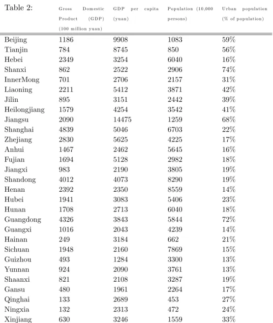
has widened continuously. This pattern is not surprising given that much of China’s recent economic development was led by rapidly expanding exports, …nanced to a considerable extent by foreign direct investment. As we can see in the Table 1 (see Appendix A.2.2), the coastal provinces concentrate more than 60 % of the GDP per capita on the whole period. Our econometrical framework will take into account such spatial heterogeneity among provinces which may a¤ect …scal policies.
Data for provinces’public expenditures come from China Statistical Yearbook in various years. Public expenditures are divided into …ve categories of spending:
o Appropriation for Capital Construction, o Expenditure for Enterprises Innovation,
o Expenditure for supporting agricultural production and agricultural operation, o Culture, Education, Science & Health Care,
o Government Administration Spending.
As you can see in the Figure 3 (see Appendix A.2.1), Social expenditures in Culture, Education, Science and Health Care represent around 40% of local government expenditures and this is the most important category of public spending since 1980. Capital expenditures also represent an important share of public spending maybe because local jurisdictions try to attract …rms and capital with infrastructures supply. Spending in enterprises innovation registers the lowest amount of expenditures (less than 10%). Expenditures for supporting agricultural production and government administration spending represent around 15% and 20% of local government expenditures. We will test the importance of strategic interactions for each category of public spending. Table 2 (see Appendix A.2.2) gives descriptive statistics for these di¤erent categories of public spending in the 29 provinces.
Local governments play an essential role in providing social services: in 2004, sub-national governments together …nanced 90 percent of public spending on education, 95 percent on health care, and 85 percent on social security. However, many local governments, espe-cially those in poor Western regions, are providing fewer and lower quality of public services. Regarding global public spending we can notice that, once again, littoral provinces, which represent 40% of the sample, concentrate 65% of local government expenditures. The dis-tribution of per capita central transfers by province in 2004 increases these inequalities:
Shanghai, the richest province, is the highest recipient of central transfers per capita (5,079 yuan) and Henan is the lowest (646 yuan), with 1117 yuan per capita. So, …scal disparity among the Eastern, the Middle, and the Western areas of China are continually enlarging. Figure 4 illustrates these disparities (see Appendix A.2.1). It con…rms that our econometrical speci…cation has to take into account spatial disparities since it appears to have important e¤ect on public spending level. We will also consider central government transfers to focus on local government public spending choices and because it may also constitutes a spatial economic shock or, more generally, an explanatory variable spatially correlated.
Finally, the level of public spending seems to be largely spatially correlated due to spatial heterogeneity or inequalities. Our empirical framework consists in testing the existence of substantive strategic interaction between Chinese local governments. We have to ascertain that the observed spatial auto-correlation can be attributed to a real strategic interaction process among jurisdictions and not to exogenous correlation in omitted provinces character-istics or common shocks to local …scal policy, which may provide false evidence of strategic interactions.
3.3 Econometric framework
Horizontal strategic interactions among Chinese provinces entail a …scal reaction function that depicts how the decision variable for a given province depends on the decisions of other provinces. To test the existence of such strategic interactions, in line of the earlier literature,34 we consider a speci…cation in which (the log of) public expenditures in province i in year t, Eit, are a function of (the log of) its neighbors public spending, Ejt. We allow
Eitto depend on a vector of speci…c controls Xitand we include a province speci…c e¤ect i.
All time-invariant community characteristics, observed or unobserved can be represented by community-speci…c intercepts. Eit= X ij ijEjt+ Xit+ i+ "it; (6) 3 4
See, for instance, Devereux, Lockwood, and Redoano (2008), Foucault, Madies, and Paty (2008) or Redoano (2007).
where i = 1; : : : ; n denotes a province and t = 1; : : : ; T a time period, ij, and are unknown parameter vectors and "it a random error.
Since there are too many parameters ij to be estimated, we estimate:
Eit = Ajt+ Xit+ i+ "it; (7)
where Ajt =
X
wij:Ejt. Eit, the vector of public spending in a local government i at time
t, depends on Ajt, the weighted average vector of public spending in the set of the other
local governments j at time t and a set of speci…c controls Xit. In our theoretical model, the
central government induces a yardstick competition among local jurisdictions with identical environments and shocks. So, we have to consider local governments which are similar, "close". A scheme that assigns weights based on geographical proximity is commonly used in the relevant empirical literature. So, …rst, we have chosen two common geographical de…nitions of neighboring communities. The …rst one is based on the Euclidean distance between jurisdictions, wdist.35 The second one is based on a contiguity matrix where the
value 1 is assigned if two jurisdictions share the same border and zero otherwise. This scheme is given by the weight matrix wcont. Moreover, following Lockwood and Migali (2009), we compare these weights to ‘placebo’weights, wplac, which are chosen in a random way without regard to any economic considerations.36 This placebo weighting scheme will give us a useful benchmark to ascertain that the potential observed spatial auto-correlation can be attributed to a substantive strategic interaction process since, if we …nd evidence of strategic interactions with the placebo matrix, which might indicate some general positive correlation between all public spending generated by omitted common shocks.37
Following Devereux, Lockwood, and Redoano (2008), Foucault, Madies, and Paty (2008), Veiga and Veiga (2007) and Redoano (2007), we introduce the lagged dependent variable, Eit 1 , as a right hand side in order to take into account the persistency in public
expendi-tures:
Eit= Eit 1+ Ajt+ Xit+ i+ "it: (8)
3 5
Weights wijare given by 1=dij where dijis the Euclidian distance between provinces i and j for j 6= i. 3 6
We generate a random number distributed between 0 and 1 for each province. Then, the value 1 is assigned if the di¤erence between random numbers of two provinces is higher than 0.5 and 0 otherwise.
3 7
Weights are normalized so that their sum equals unity for each i for all weight matrices. This assumes that spatial interactions are homogeneous: each neighbor has the same impact on the province.
Lastly, we introduce a trend variable and speci…c control variables to ascertain that the observed spatial auto-correlation can be attributed to a substantive strategic interaction process and not to exogenous correlation in omitted provinces characteristics or common shocks to local …scal policy,
Eit= Eit 1+ Ajt+ 1Pit+ 2Git+ 3Uit+ 4Oit+ 5Fit+ 6Cit+ 7Tt+ i+ "it; (9)
where Eit is per capita expenditures of province i on year t, Eit 1 is the lagged value of our
dependent variable, Ajt is the weighted average vector of per capita public spending in the set
of the other local governments j at time t.38 We add some speci…c control variables to avoid the omission of explanatory variables that are spatially dependent and may generate spatial error dependence: Pitis the population of jurisdiction i on year t, which captures the
possibil-ity of scale economies in public spending, Git is the Gross Domestic Product (GDP) growth
rate in province i on year t; an indicator of the economic conjuncture which allows control-ling for common shocks spatially correlated, Uit is the share of urban population in the total
provinces population, knowing that urbanization is spatially distributed and may increase public spending needs in particular in terms of infrastructures (Guillaumont Jeanneney and Hua (2001), Rodrik (1998)), Oit is a trade openness measure at provincial level which could
have many e¤ects on public …nances,39 as well as Fit, the foreign direct investment in‡ow in
province i on year t. Cit is the central government transfers for province i on year t and Tt
is a trend variable which captures common trend for all provinces.40 Note that the central government transfers are introduced only as robustness check because of the lack of data.41
In estimating this reaction function we are confronted to important econometric issues
3 8 Per capita expenditures and population are in log. 3 9
Rodrik (1998) shows that there exists a positive correlation between an economy’s exposure to inter-national trade and the size of its government because government spending plays a risk-reducing role in economies exposed to a signi…cant amount of external risk. As Combes and Saadi-Sedik (2006) have shown, even if trade openness increases a country’s exposure to external shocks and thereby adversely a¤ects its budget balances, an outward looking policy strategy should lead to an overall strengthening of its budget balance.
4 0 We can’t introduce time dummies since we use GMM System with external instruments and we have
too many instruments with time dummies. However, this is a good way to ascertain that the potential observed spatial auto-correlation can be attributed to a substantive strategic interaction process and not to a “common trend”. Indeed, Manski (1993) suggests that …scal choices appear to be interdependent not because jurisdictions behave strategically but because they actually follow a “common trend”that drives …scal choices in the same directions.
4 1
(Brueckner (2003)).
First, as said before, the omission of explanatory variables that are spatially dependent may generate spatial dependence in the error term, which is given by: "it= w"it+ vit:
When spatial error dependence is ignored, estimation can provide false evidence of strategic interactions. To deal with this problem, one possible approach is to use the ML estimator, taking into account the error structure or the IV method which yields consistent estimations even with spatial error dependence (see Kelejian and Prucha (1998)).42 Brueckner and Saavedra (2000), Saavedra (2000) or Foucault, Madies, and Paty (2008) use the tests of Anselin, Bera, Florax, and Yoon (1996) to verify the hy-pothesis of error independence. We can note that the use of panel help eliminate spatial error dependence which arises through spatial autocorrelation of omitted variable which are time-invariant.
Secondly, because of strategic interactions, public expenditures in di¤erent provinces are jointly determined: if local governments react to each others’ spending choices, neighbors’ decisions are endogenous and correlated with the error term "it. In this
case, ordinary least squares estimation of the parameters are inconsistent, requiring alternative estimation methods based on the instrumental variables (IV) method or on the maximum likelihood (ML). Under IV approach, a typically procedure is to use the weighted average of neighbors’control variables as instruments (Kelejian and Prucha (1998)). The ML method consists in using a non-linear optimization routine to estimate the spatial coe¢ cient (Brueckner (2003)).
Lastly, since we introduce the lagged dependent variable as a right hand side to consider the autoregressive component of the time series, the previous estimators are inconsistent (Nickell (1981)).
We propose to use the GMM-System estimator in addition to the IV estimator of the spatial coe¢ cient, after verifying the hypothesis of error independence and estimating the
4 2Case, Rosen, and Hines (1993), Besley and Case (1995b), Brueckner (1998) and Brueckner and Saavedra
(2000) use the maximum likelihood approach. Brett and Pinkse (1998), Heyndels and Vuchelen (1998), Figlio, Kolpin, and Reid (1999) and Buettner (2001) are examples of empirical studies that use the IV approach to estimate spatial coe¢ cients.
static model with ML estimator. As for the neighbors’ spending decisions, following Re-doano (2007), Devereux, Lockwood, and ReRe-doano (2008) and Foucault, Madies, and Paty (2008), we use the weighted average of neighbors’control variables, i.e., their socio-economic characteristics (wijXjt), as instruments. The GMM estimators allow controlling for both
unobserved country-speci…c e¤ects and potential endogeneity of the explanatory variables.43 The GMM-System estimator combines in one system, the regressions in di¤erence and the regressions in level. Blundell and Bond (1998) show that this extended GMM estimator is preferable to that of Arellano and Bond (1991) when the dependent variable, the independent variables, or both are persistent.
3.4 Public spending interactions and strategic complementarity
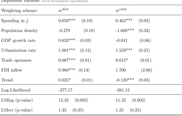
To investigate whether spatial lag or spatial error dependence are the more likely sources of correlation, we use two robust tests based on the Lagrange Multiplier principle for panel data that indicate what is the most likely source of spatial dependence (Anselin, Le Gallo, and Jayet (2006)). We compute these robust tests for spatial lag dependence and for spatial error dependence. As you can see in the Table 3 (see Appendix A.2.3), spatial tests indicate the presence of spatial lag dependence for public spending but not the existence of spatial error dependence for both matrices. As the hypothesis of error independence is veri…ed, we estimate the equation (9) using ML with speci…c-e¤ects for both contiguity and distance matrices without taking into account the lagged value of our dependent variable ( = 0). The estimation results are shown in Table 3. In these …rst estimations, the coe¢ cient of the weighted average vector of public expenditures in the set of other local governments is always signi…cant and positive, for both matrices.
We then estimate with GMM-System the dynamic model (equation 4) for both weighting schemes taking into account the lagged value of our dependent variable ( 6= 0). We adopt the assumption of weak exogeneity of GDP growth rate, trade openness, foreign direct investment in‡ow and central government transfers and the assumption of strict exogeneity of other
4 3
There are conceptual and statistical shortcomings with the …rst-di¤erence GMM estimator as it exacer-bates the bias due to errors in variables (Hausman, Hall, and Griliches (1984)). Thus, we use an alternative system estimator that reduces the potential biases and imprecision associated with the usual di¤erence esti-mators (Arellano and Bover (1995) and Blundell and Bond (1998)) and also greatly reduces the …nite sample bias (Blundell, Bond, and Windmeijer (2000)).
explanatory variables.44 As noted before, the weighted average vector of per capita public spending in other provinces is also instrumented by the weighted average of neighbors’control variables. We collapse instruments and limit its number since too many instruments leads to inaccurate estimation of the optimal weight matrix, biased standard errors and, therefore, incorrect inference in overidenti…cation tests (see Roodman (2009)).45 Table 4 shows these estimation results for distance matrix and Table 5 for contiguity matrix (see Appendix A.2.3). The consistency of GMM-System estimator is given by two speci…cation tests (Arellano and Bond (1991)). With the Hansen test, we cannot reject the null hypothesis of the overall validity of instruments’orthogonality conditions. The second tests concern the serial corre-lation of residuals: we reject the null hypothesis of no …rst-order serial correcorre-lation and do not reject the null hypothesis of no second-order serial correlation of di¤erenced residuals. So, we conclude that orthogonality conditions are correct and instruments used valid. We introduce the control variables progressively to check the robustness of our results.
We can note …rst that the coe¢ cient on lagged dependent variable is always signi…cant and positive. As this coe¢ cient provides an estimated varying between 0.45 and 0.89 signi…cant at 1% level, the result indicates persistency of public expenditures and con…rms the consistency of the autoregressive speci…cation.
The coe¢ cient of the weighted average vector of public expenditures in the set of other provinces is signi…cant at least at 5% level and positive for both matrices. Moreover, it is robust and relatively stable with the introduction of the control variables. However, if we continue to …nd evidence of strategic interactions with the placebo matrix, that might indicate some general positive correlation between all public spending generated by omitted common shocks. It would cast doubt on our claim that we have found evidence of public spending interactions. But, we see from Table 5 on the last column, that placebo matrix do not show any evidence of positive strategic interactions. This shows that the phenomenon of …scal interactions detected with geographical matrices is not an artefact of the estimation procedure. So, we can conclude that there are some strategic interactions between Chinese
4 4 Population density, trend and urbanization rate. 4 5
The lags of at least two periods earlier for weak exogenous variables and three periods earlier for en-dogenous variables are used as instruments. The lagged dependent variable is instrumented by lags of the dependent variable from at least two periods earlier.
We use two lags for endogenous and weak exogenous variables. Note that we consider external instruments as weak exogenous but we use only one lag when the number of instruments exceeds the number of units.
provinces and public expenditures seem to be strategic complements: an average public spending increase of 10% in the neighboring provinces induces an increase of around 5,9% with the distance matrix and 2,8% for with contiguity matrix in provincial expenditures.
As expected, the parameter associated with population is negative and signi…cant: it indicates the presence of scale economies in public spending. We …nd a positive and signi…cant sign for the parameter associated with the GDP growth rate, which indicates the e¤ect of economic conjuncture. Results also tend to show that urbanization actually increases public spending needs. The coe¢ cient associated with the central government transfers is also positively correlated with the level of public expenditures, as it is generally the case for trade openness. However, the coe¢ cient of foreign direct investment in‡ow is, for the most part, non signi…cant.
Since, in China, the central government considers di¤erent groups of provinces (coastal, south. . . ) in these economic reforms, the competition may also appear among provinces which belong to the same group. Moreover, among these groups, provinces have generally the same characteristics so that governors can be compared. So, we also consider a weighting scheme (wreg) where the value 1 is assigned if two jurisdictions belong to the same group and zero otherwise.46 However, as you can see in the Table 6 (see Appendix A.2.3), results are similar with the contiguity matrix.47
Finally, our results provide evidence for the existence of horizontal strategic interactions and the strategic complementarity of public spending among "close" Chinese provinces. We can notice that this result is close to those obtained in previous tests carried out in other countries.48
We extend our empirical analysis by testing the existence of horizontal strategic inter-actions for each category of public spending. Indeed, Case, Rosen, and Hines (1993) and
4 6
Beijing, Tianjin, Hebei, Shanxi and InnerMong belong to the “North”, Liaoning, Jilin and Heilongjiang to the “Northeast”, Shanghai, Jiangsu, Zhejiang, Anhui, Fujian, Jiangxi and Shandong to the “East”, Henan, Hubei, Hunan, Guangdong, Guangxi and Hainan to the “South Central ”, Sichuan, Guizhou and Yunnan to the “South West” and Shaanxi, Gansu, Qinghai, Ningxia and Xinjiang to the “North West”.
4 7 That’s not surprising since the correlation coe¢ cient between the weighted average vector of public
spending with the two matrices is 0.96.
4 8The empirical evidence of public spending interactions and their strategic complementarity relates to the
United States (Case, Rosen, and Hines (1993), Figlio, Kolpin, and Reid (1999)), European counties (Redoano (2007)), Indonesia (Arze, Martinez-Vasquez, and Puwanti (2008)) or French municipalities (Foucault, Madies, and Paty (2008)). For empirical evidence of yardstick competition see Besley and Case (1995b) for United States), Ashworth and Heyndels (1997) for Flemish Belgium, Bordignon, Cerniglia, and Revelli (2003) for Italy, Schaltegger and Kuttel (2002) for Switzerland and Revelli (2006) for the United Kingdom.
Foucault, Madies, and Paty (2008) suggested that there is no reason to assume that pat-terns of expenditures interdependence are identical for all categories of public spending. Results are provided in Table 7 and 8 (see Appendix A.2.4) for distance and contiguity ma-trix. Regarding coe¢ cients associated with weighted average vector of public expenditures in neighboring provinces for the various categories of public spending, we notice that public spending interactions seem to be strongest and most signi…cant for the category "appropria-tion for capital construc"appropria-tion" and for "expenditures for enterprises innova"appropria-tion". Estima"appropria-tions provide estimated coe¢ cients varying between 0.35 and 0.24, signi…cant at 1% level with the distance matrix. This result may re‡ect competition among Chinese provinces to attract …rms and capital with infrastructures supply, which is an important indicator of performance for the central government. We have similar result with Foucault, Madies, and Paty (2008) who found a higher coe¢ cient for investment expenditures and argued that there are spend-ing interactions between neighborspend-ing French municipalities for the most “visible” category of expenditures. Strategic interactions are smaller for local social expenditures ("culture, education, science & health care"). Lastly, results provide no evidence for expenditures for supporting agricultural production and local government administration spending.
Finally, strategic interactions vary according to categories of public expenditures and results seem to re‡ect competition among local governments to attract …rms with infrastruc-tures supply, resulting from a yardstick competition created by the central government.
3.5 Decentralization degree and strategic interactions
As said before, according to the corollary 1, when the …scal system is centralized, local o¢ cials do not care about what other local governments are doing so that we should not have any horizontal strategic interactions. We cannot test directly this hypothesis since we lack of data for the period before the decentralization. So, we propose to test the e¤ect of the decentralization degree on the existence of horizontal strategic interactions. The horizontal strategic interactions should be higher, the higher the decentralization degree is.
decentralization degree (Decit) and we estimate:
Eit= Eit 1+ 0Ajt+ 00(Ajt Decit)+ 1Pit+ 2Git+ 3Nit+ 4Oit+ 5Uit+ 6Tt+ 7Decit+ i+"it;
(10) If the decentralization actually reinforces strategic interactions, we should observe the coe¢ cient 0 and 00 being both signi…cantly positive. Following the relevant literature,49 we choose two usual approximations of …scal decentralization: subnational expenditure as a percentage of national expenditure and transfers from central government as a percentage of subnational government revenue.50
Table 9 (see Appendix A.2.5) gives the estimation results for both matrices. Our results tend actually to show that public spending interactions are reinforced by the …scal decen-tralization. Indeed, for both matrices, coe¢ cients associated with Ajt and (Ajt Decit) are
signi…cantly positive with the …rst approximation of …scal decentralization (column (1) and (2)).51 There are horizontal strategic interactions among local governments which are com-plements and reinforced by a higher degree of decentralization. These results are consistent with those of Huther and Shah (1998), Barenstein and de Mello (2001) and Fisman and Gatti (2002) who all report that a larger subnational share of public expenditures was asso-ciated with lower corruption and those of Treisman (2000) and Arikan (2004) who explored whether smaller local units were associated with less corruption because of more intense interjurisdictional competition.
As robustness test, as said before, we use an alternative approximation of …scal decen-tralization and evaluate the e¤ect of the transfers from central government as a percentage of subnational government revenue on the existence of strategic interactions in column (3) and (4). It can be considered as an indicator of degree of dependence and a sign of weakness in terms of subnational resources. As expected, on the contrary, public spending interactions are reduced by "…scal centralization". Indeed, central government transfers have a positive e¤ect
4 9In particular, Huther and Shah (1998), Barenstein and de Mello (2001), Fisman and Gatti (2002), Arikan
(2004), Rodríguez-Pose and Krøijer (2008) or Enikolopov and Zhuravskaya (2007) in their studies of the e¤ects of …scal decentralization on governance, corruption, growth and political institutions.
5 0 More precisely, we use the ratio of jurisdictions’ public spending per capita over the total central
gov-ernment public spending per capita, for each jurisdiction and the share of central govgov-ernment transfers per capita relative to local revenue per capita of the local government.
5 1
on the level of public spending in provinces but it reduces interjurisdictional competition: the coe¢ cient associated with the interaction between the neighbors’ spending decisions (Ajt)
and an indicator of centralization (Cit) is signi…cantly negative while coe¢ cients associated
with (Ajt) and (Cit) are both positive.
Finally, …rst, our empirical work provides evidence for the existence of horizontal strategic interactions and the strategic complementarity of public spending among Chinese provinces which is consistent with the corollary 2 of our theoretical model. We have also shown that strategic interactions vary according to categories of public expenditures and results seem to re‡ect competition among local governments to attract …rms with infrastructures supply, resulting from a yardstick competition created by the central government. Second, our results tend to show that the horizontal strategic interactions are higher, the higher the decentralization degree is, as we can expect from the corollary 1 of our theoretical work.
4
Conclusion
Some scholars argue that …scal decentralization in China was the key for Chinese remarkable growth, by creating strong incentives to promote local economic growth. However, "Chi-nese style decentralization" is conceptually di¤erent from the decentralization in many other countries. In particular, there is a divergence between the assumptions of orthodox …scal federalism theory and the institutional and economic realities in China. Indeed, China’s cur-rent …scal system is largely decentralized while its governance structure is rather centralized, the power of provincial governments is not based on a system of electoral representation and the population mobility is limited. Here, following Blanchard and Shleifer (2000), we argue that, when disciplining devices such as local election and the exit option are far from perfect, vertical control can ensure local accountability. Under this centralized political system, the government can create a yardstick competition among local o¢ cials by rewarding or punish-ing them on the basis of economic performance like voters do in democratic countries (Besley and Case (1995b)).
So, we have developed a model of public spending setting in a multijurisdictional world with asymmetric information, where the central government makes comparisons between