HAL Id: hal-01719101
https://hal.archives-ouvertes.fr/hal-01719101
Preprint submitted on 27 Feb 2018
HAL is a multi-disciplinary open access
archive for the deposit and dissemination of sci-entific research documents, whether they are pub-lished or not. The documents may come from teaching and research institutions in France or abroad, or from public or private research centers.
L’archive ouverte pluridisciplinaire HAL, est destinée au dépôt et à la diffusion de documents scientifiques de niveau recherche, publiés ou non, émanant des établissements d’enseignement et de recherche français ou étrangers, des laboratoires publics ou privés.
Influence of Tipping Points in the Success of
International Fisheries Management: An Experimental
Approach
Jules Selles, Sylvain Bonhommeau, Patrice Guillotreau, Thomas Vallée
To cite this version:
Jules Selles, Sylvain Bonhommeau, Patrice Guillotreau, Thomas Vallée. Influence of Tipping Points in the Success of International Fisheries Management: An Experimental Approach . 2018. �hal-01719101�
1
Influence of Tipping Points in the Success of International Fisheries
1
Management: An Experimental Approach
2 3
Selles Jules1,3*, Bonhommeau Sylvain2, Guillotreau Patrice3 and Vallée Thomas3 .
4 5
1IFREMER (Institut Français de Recherche pour l’Exploitation de la MER), UMR MARBEC, Avenue Jean 9
6
Monnet, BP171, 34203 Sète Cedex France. 7
2IFREMER Délégation de l’Océan Indien, Rue Jean Bertho, BP60, 97822 Le Port CEDEX France.
8
3LEMNA, Université de Nantes, IEMN-IAE, Chemin de la Censive-du-Tertre, BP 52231, ´44322 Nantes Cedex
9
France. 10
*corresponding author, email: jules.selles@gmail.com, tel: +33 (0)779490657 11
12
Abstract —International fisheries are common pool resources which concentrate management difficulties. 13
The migratory nature of fish resources makes it available for a large number of actual and potential harvesters 14
in high seas which are by nature, free of access. This work investigates the role of critical socio-economic 15
tipping points on cooperation during the policy-making process associated with international shared fisheries. 16
We analyze the ability of decision makers to coordinate their decisions to reduce economic rent dissipation 17
and to ensure resource sustainability in a dynamic environment. More specifically, we propose a 18
contextualized computer-based experimental approach to explore how decision makers respond to an 19
endogenously driven catastrophic change in the economic conditions. We use the study case of the East 20
Atlantic bluefin tuna (EABFT) fishery as it has been the archetype of an overfished and mismanaged fishery. 21
We show that the threat of a regime shift, by increasing the likelihood of an economic bankruptcy, fosters 22
more cooperative outcomes and a more precautionary management of the resource. This result is exacerbated 23
when the position of the tipping point which triggers the shift in economic condition is uncertain. 24
25
Keywords— Experimental economics; Fisheries management; Common pool resources, Tipping points; 26
International fisheries; Policy making. 27
2
1.
Introduction
29
Fishery resources are common-pool resources (CPRs), in which appropriation (catch) of the 30
resource by one fisher creates an external cost for others. In such a context, the incentives to 31
catch more resources and ignore the external costs are rational because a fisher receives 32
benefits for himself without bearing the social costs. Collectively, this rational individual 33
behavior leads to the well-known tragedy of the commons (Gordon 1954; Hardin 1968). 34
Fisheries management has faced difficulties all over the world for the second half of the 20th 35
century and the beginning of this century to address both conservation and economic challenges 36
(Pauly et al., 1998; Worm et al., 2009). Scientists have pointed out the poor governance practices 37
and deficient incentives for conservation (Hilborn et al., 2005). 38
International fisheries in the high seas are a special case which causes particular management 39
problems. International shared fish stocks are defined as fish stocks not confined to a single 40
national jurisdiction (Economic Exclusive Zone, EEZ), and exploited by more than one State 41
(Munro, 2004). Compared to domestic fisheries, international fisheries are subject to 42
management difficulties mainly due to the need for cooperation between different countries 43
(Munro 1979, Munro et al., 2004, Maguire et al., 2006, McWhinnie 2009, Teh & Sumaila, 2015). 44
Inadequate management has led to overfishing of many economically important fish stocks 45
(Cullis-Suzuki & Pauly, 2010). Highly migratory fish stocks represent the most complex case of 46
international fisheries. The highly migratory nature of such fish resources makes it available for 47
a large number of actual and potential harvesters in high seas which are by nature free of access 48
(White & Costello 2014). Nowadays, the current status of a number of highly migratory stocks 49
(mainly tuna and tuna-like species) is particularly worrying (Juan-Jorda et al., 2011). Since the 50
1995 United Nations Fish Stocks Agreement, highly migratory species have been managed on a 51
regional basis through Regional Fisheries Management Organizations (RFMOs). The RFMOs are 52
composed of members from both coastal states and distant water fishing nations (DWFNs). 53
Despite the legal obligation to cooperate within a RFMO, the states involved in international 54
fisheries are not required to reach an agreement, or if an agreement is achieved, it is not binding 55
or enforceable (Munro et al., 2004). This means that non-cooperation is the default option, 56
notably in front of the complexity to manage highly migratory species and reach stable 57
agreements. 58
An example is given by the East Atlantic and Mediterranean stock of bluefin tuna (EABFT), a 59
highly migratory species. Until 2009, the stock has been deemed an archetype of 60
overexploitation and mismanagement (Fromentin et al., 2014). Several countries, both coastal 61
and DWFNs, have contributed to a high level of exploitation driven by the high market value of 62
the tuna on the Japanese market (Fromentin et al., 2014). The decline in the EABFT stock has 63
3
raised considerable concerns about its management (ICCAT, 2007, Hurry et al., 2008, ICCAT, 64
2009). Under the governance of the International Commission for the Conservation of Atlantic 65
Tunas (ICCAT), the fishery has suffered both from its failure to follow the scientific advice and a 66
high level of illegal, unreported and unregulated (IUU) fishing. This situation has occurred since 67
the establishment of the first management regulation based on quotas (Total Allowable Catch, or 68
TAC) in 1999 and lasted until 2009. At this period of time, the objective to reach the Maximum 69
Sustainable Yield (MSY) was far from being achieved. It is only under the threat by 70
environmental Non-Governmental Organizations (NGOs) to propose listing EABFT in Appendix I 71
of CITES (Convention on International Trade in Endangered Species of Wild Fauna and Flora) 72
which would have prohibited any international trade for this species, that ICCAT established a 73
recovery plan for EABFT since 2009. For the very first time, ICCAT has fully endorsed scientific 74
advice and reached an agreement to considerably reduce the fishing effort and allowable catch 75
as well as implementing some management measures (e.g., size limitations, fishing seasons). 76
Game theory offers important results about the outcomes of non-cooperative harvest (since the 77
seminal work of Munro 1979, Levhari & Mirman, 1980 and Clark 1980) and the benefits to reach 78
and maintain cooperative agreement in the context of international fisheries (e.g., Brasao et al., 79
2000, Pintassilgo et al., 2003, 2010, 2015; for a review see Bailey et al., 2010, Hannesson 2011, 80
and Sumaila 2013). However most of the game theory applications in fisheries exclude complex 81
resource dynamics or potential changes in the management framework (Bailey et al., 2010). 82
As observed in the case of the EABFT fishery, society and public opinion put pressure on RFMOs 83
to address urgently such complex problems, particularly if they perceive a risk of critical 84
threshold to be exceeded. Beyond a critical threshold, management systems can switch swiftly 85
to a high action level with new management frameworks and paradigms (Scheffer et al., 2003). 86
This is the parallel of regime shifts in ecology which are large, abrupt and persistent changes in
87
the structure and function of an ecosystem (Biggs et al., 2012). The point where the shift occurs 88
is called a tipping point. The effects of such tipping points could play an important role in the 89
management of common resources in a high hierarchical and centralized institution, such as the 90
ICCAT or the European Union (EU). The political management systems propose very few 91
incentives to achieve the long term sustainability of stocks (Daw & Gray, 2005). Moreover, 92
stakeholders impacted by ecosystem management may prefer some stability and avoid 93
continuous and costly changes in management recommendations (Armsworth & Roughgarden 94
2003, Patterson & Resimont 2007, Boettiger et al., 2016). Drastic adjustments to reach stocks 95
sustainability are often taken only once the state of the resources has called society attention 96
(e.g EABFT fishery case in Fromentin et al., 2014). 97
An empirical method to explore conditions of cooperation in a complex socio-economic system, 98
such as international fisheries, relies on laboratory experiments. Experimental studies on CPRs 99
4
have proven to test effectively the impact of specific variables in repeated controlled settings 100
(Ostrom 2006). Our objective is to analyze the ability of decision makers to coordinate their 101
decisions in order to reduce economic rent dissipation and to ensure resource sustainability in a 102
dynamic environment. In the present research work, we assess the cooperation in response to 103
the introduction of endogenous socio-economic tipping points with or without uncertainties. 104
The socio-economic shift considered in this study is a latent and endogenous cost driven by 105
collective actions (aggregated catches). We design our experiment to the case study of the 106
EABFT exploitation following Brasao et al., (2000). Subjects, who are representatives of identical 107
States, are involved in the EABFT fishery management by defining their own catch level 108
(quotas). Our approach can be applied to a variety of CPR situations and collective action 109
problems (Ostrom, 2006, Poteete et al., 2010, Anderies et al., 2011), but our focus in this paper is 110
on ensuring sustainable exploitation of fish stocks. . 111
Using a dynamic CPR game framework, Lindahl et al., (2016) already studied how the 112
introduction of an ecological tipping point affects the productivity of the resource affects, hence 113
the profitability of CPR users. They showed that a group of users manages a resource more 114
efficiently when confronted to a latent abrupt change. Schill et al., (2015) extended these results 115
by showing that the threshold impact on resource utilization is observed only in situations 116
where the likelihood of the latent shift is highly probable. We extend the experimental work of 117
Lindahl et al., (2016) by testing the effect of the inclusion of a tipping point affecting the 118
economic conditions of the dynamic game in which subjects decisions are based on economic 119
outcomes. We also extend the work of Schill et al., (2015) by analyzing how the position of a 120
latent shift affects resource management instead of analyzing the effects of the occurrence 121 probability. 122
2.
Experimental setting
123 2.1. Experimental design 124Research questions are tested using a modified version of the experimental design of Mason & 125
Philips (1997). This protocol defines a CPR request game (Budescu et al., 1995), in which a few 126
firms harvest a resource in a dynamic context. We adapt their oligopoly model to a situation 127
where the price is exogenously determined (constant price) and include a critical tipping point 128
in the resource level which affects the economic conditions of the game. Following the 129
methodology used in other complex ecological dynamic experiments (Schill et al., 2015, Lindahl 130
et al., 2016), we introduce a non-neutral framework. The task and information given to subjects 131
correspond to a stylized representation of the actual context of the ICCAT decision committee. 132
The subjects are asked to define their harvest levels (quotas) for the East stock of Atlantic 133
5
Bluefin tuna, instead of collecting tokens (Harrison and List 2004 for a characterization of 134
experiments). Subjects are only able to communicate through a non-binding pledge process: face 135
to face communication is not allowed. Moreover, to approximate an infinite time horizon super-136
game, the subjects do not know the number of rounds to be played1; they only know the
137
maximum duration. However, we make sure to end the experiment early enough to avoid 138
potential end game effects. 139
We align our experiment onto the model of Hannesson (1997). The yearly CPR biomass 140
dynamics (Bt) is modeled by a logistic growth (1) subject to fishing (Yt). 141
B = G B − Y (1)
142
With theyear and G B = round B . 1 + r. 1 − !"!. 143
We assume that the marginal cost of fishing (c) is inversely proportional to the size of the stock 144
at any point in time2.The total cost (C) in period t will then be:
145
C B = $' () %& dx = c. ,ln.G B
/ 0 − ln B 1 (2)
146
The fish harvest Yt caught in period t could be described by 2 34/ – Bt. At a given constant 147
price (p), the total profit (54) obtained by all players (i) in period t with a fixed cost (6) 148
associated with an endogenous resource threshold Blim. will be: 149
7π = p. Y − C B , for B ≥ Bπ = p. Y − C B − α. N, for B < B=>?
=>? (3)
150
With N the number of participants, and assuming constant return to scale, the individual profit is 151
π>, = p. y>, − C B .CED,, for B > B=>? and π>, = p. y>, − C B .CED, – α, for B ≤ B=>?.
152
We introduce a fixed cost related to the resource size beyond the threshold level. This cost is a 153
stylized representation of the critical effect of resource depletion. In the case of the EABFT 154
fishery, this cost represents the effect of a ban on the species commercial exchange. This fixed 155
cost formulation follows the assumptions from public good games with potential catastrophic 156
effects of climate shifts (Milinski et al., 2008, Barret & Danenberg 2012, 2013). 157
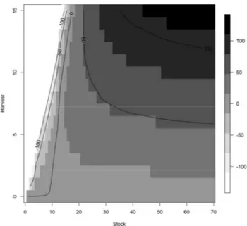
We introduce the resource growth model as a discrete function to our subjects (Figure 1) and 158
the associated profit evolution as depending on the stock and catch levels (Figure 2) for a 159
selection of parameters that fit the context of EABFT (stylized version, Table 1). The minimum 160
resource size allowing for reproduction is 3 units (1 unit is equivalent to 104 tons) and the
161
maximum resource size is set to 70 units. The maximum sustainable yield (MSY) is 3 units for a 162
stock size between 28 to 42 units. The profit is maximum, greater than 100 units (1 monetary 163
unit is equivalent to 107 €), when both the stock and catch levels are maximum, then it steadily
164
1 As in Lindahl et al., (2016), to ensure an unknown time horizon, we varied the end-time between and within groups. 2 This cost function implicitly assumes that the cost per unit of fishing effort is constant and the catch per unit of effort
6
decreases until the stock reaches the lowest values and becomes null at any catch level for a 165
stock size of 10 units. In all treatments, the groups start with a stock size of 52 units and over a 166
number of periods unknown to them, they harvest resource units restricted by an individual 167
capacity constraint of 5 units (yi,t=[0,1,2,3,4,5]). Groups are composed of 3 subjects sharing the
168
same characteristics. This design follows the stylized representation from a game theory model 169
of the EABFT fishery (Brasao et al., 2000). 170
171
Figure 1: Profit (107€) as a function of stock (104 tons) and harvest level (104 tons).
172
173
Figure 2: Logistic resource growth (104 tons).
174
175 176
7
Table 1: Bioeconomic model parameters.
177
Variable Description Value
N Participant number 3
ymax Maximum harvest [104t] 5
p Price [107€/104t] 10
r Growth rate 0.15
K Carrying capacity [104t] 70
c Cost parameter [107€/104t] 100
α Threshold fixed cost [107$] 30
Blim Threshold [104t] 20
178
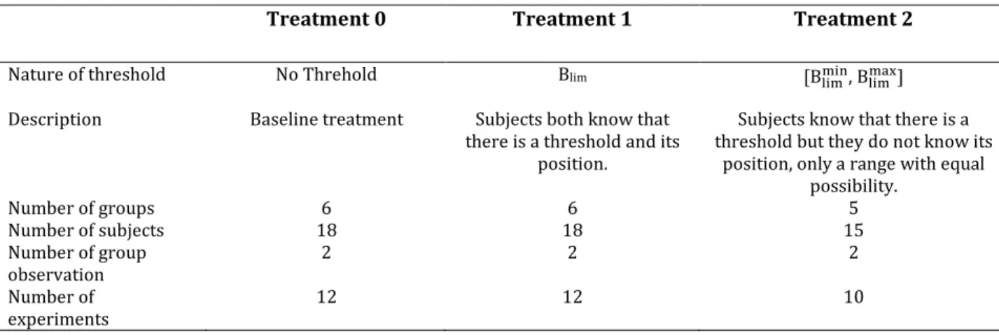
We introduce three experimental treatments to assess the cooperation in response to the 179
introduction of three kinds of endogenous socio-economic tipping points: i) base case without 180
tipping point; ii) known tipping point and iii) uncertain (localized) tipping point. In all three 181
experimental treatments (T0, T1 and T2 in Table 2), a group of subjects defines a catch harvest 182
for their own EABFT fishery. The only aspects that differ between treatments are the nature of 183
the threshold (Blim). The uncertainty surrounding the latent endogenous shift differs from the 184
risk evaluated by Schill et al., (2015). In our case, the uncertainty focuses on the position of the 185
threshold, and not on its existence. The third treatment (T2) introduces uncertainty around the 186
position of the threshold value Blim which is drawn within a 40% uncertainty range [3HIJJIK, 3HIJJLM]
187
centered around the value of Blim3.
188 189
Table 2: Experimental design.
190
Treatment 0 Treatment 1 Treatment 2
Nature of threshold No Threhold Blim [B=>??>N, B=>??O&]
Description Baseline treatment Subjects both know that
there is a threshold and its position.
Subjects know that there is a threshold but they do not know its
position, only a range with equal possibility. Number of groups 6 6 5 Number of subjects 18 18 15 Number of group observation 2 2 2 Number of experiments 12 12 10 2.2. Experimental procedure 191
The experiment was conducted at the experimental laboratory of the University of Montpellier 192
(LEEM) with a total of 51 subjects drawn from the undergraduate student population in May 193
2017. The experiment was conducted through a computer-based approach realized with the 194
oTree software (Chen et al., 2016). Each experimental session lasted a maximum of two hours 195
8
with two repetitions of the game for the same group of subjects (phases). Participants received a 196
show-up fee of 6 € and the average earnings during the experiments were 2.94 €, paid privately 197
at the end of the experiment. 198
When the subjects arrived, they signed a consent form and were randomly assigned to a group of 199
3 subjects with the instructions to read (Appendix A). They were told that each subject 200
represented a country, and that, together with the two other participants of their group, they 201
had access to the stock of the East Atlantic bluefin tuna, a common renewable resource, from 202
which they had to decide the amount of allowable harvest for their fishery at the beginning of 203
each round (each year), before deciding privately in a further step what would be their own 204
harvest decision. Subjects were told that the experiment would end either when the stock is 205
depleted or when the experimenter decides to stop it, but the exact end-period was unknown to 206
them. They began with a capital of 50 monetary units and were paid proportionally to their 207
accumulated profit during the experiment with a rate of 1 unit equal to 0.05€ plus an additional 208
revenue of 0.2€ for correct belief elicitation. Belief elicitation constitutes a guess of the 209
expectation of other subjects’ behaviour (harvest level). They received payment for only one 210
phase of the experiment randomly chosen and unknown to them. No direct communication (face 211
to face) between subjects was allowed. 212
Before the start of the experiment, the subjects were asked to fill out a form to inform their 213
identity and if they were concerned or involved with the subject of the study (Appendix B), and 214
then they were tested for their understanding of the instructions, i.e. resource dynamics and 215
profits (3 questions, Appendix B). Any remaining question was answered by the experimenter. 216
For each round, players received information about the resource state from which a profit table 217
is derived and updated for every round (Appendix C). They were also informed about the 218
percentage variation of the biomass for the next year through a variation table depending on the 219
harvest level of the group (Appendix C). Furthermore, the mean resource level at MSY (35 units) 220
was also indicated with the resource status and defined as a non-binding objective for the group. 221
This information creates a collective reference point in order to facilitate the understanding of 222
the long term sustainable resource level maximizing the growth of the resource. Therefore, 223
optimizing the use of the resource can focus on the mere level ensuring maximum profits. This 224
information is necessary to concentrate the problem on the resource sharing issue, and not on 225
the optimization of a non-linear dynamic system which proved to be a complex problem 226
(Moxnes, 1998 and Hey et al., 2009). 227
On top of deciding their harvest level, the subjects had to guess the sum of harvest units they 228
expected the other players would harvest in each period from 0 to 10 units. Belief elicitation was 229
incentivized with a payoff of 0.2 € for good prediction and allowed examining the source of 230
deviations from theoretical predictions. Thereafter, participants pledged an amount of catch 231
9
they would harvest individually. It was common knowledge that these declarations were non-232
binding but would be communicated to the group. After these declarations were revealed, the 233
participants chose simultaneously their actual harvest level for the round (year). At the end of 234
the round, the participants were then informed about everyone’s decisions for the round and 235
they were given their cumulated profit and the track records of the total catch, profit and own 236
decision during the game. They also had access to a projection of the future resource status 237
assuming a constant harvest level scenario defined at the current harvest level (Appendix D). At 238
the end of the experiment, participants were informed about their cumulated profit. They were 239
also asked to indicate, on a five-point Likert scale, to what extent they understood the resource 240
dynamics and the cooperation level of their group during the experiment. 241
2.3. Formulating hypothesis
242
To formulate the research hypotheses, we rely on the analysis of an indefinite time horizon 243
supergame made by Hannesson (1997). The subjects know that the game will end at some point 244
but not when. At every round of the game, each subject i in the group has an individual 245
perception about whether or not the game would last another round (sort of a discount factor), 246
which we denote PI (Fudenberg and Tirole 1998). The implication of these subjective 247
probabilities defines the equilibrium conditions of the game. 248
During the experiment, participants receive updates on the stock level Bt and on their available 249
profit at the beginning of each period. They also know if someone deviates from its proposition 250
and if a participant behaves as a selfish agent. Thereby, each participant conditions his strategy 251
on past and current resource and profit levels. On the basis of this information, each participant 252
plays a Markov strategy (Maskin and Tirole 2001). Because players are symmetric (same cost 253
functions), we only consider equal sharing equilibria (equal share of the resource) in which each 254
subject gets Q of the total profits of each period. 255
Cooperative strategy could be sustained by a trigger strategy in the game. Considering the case 256
without tipping point, if one of the participants deviates from the optimal solution, she/he would 257
gain more in the current period and would then be punished afterwards. Other players would 258
retaliate by fishing down the stock in the following periods until further depletion becomes 259
unprofitable. Such a scenario results in resource depletion until the marginal cost of fish caught 260
(R) is equal to the marginal revenue, i.e. the fish price (p, Eq. 3). The size of the stock resulting 261
from such a strategy is then: 262
BS=T% (4)
263
Otherwise, the optimal solution could be sustained as a Markov perfect strategy if the defection 264
is not profitable. The net present value of the cooperative strategy, UVWX, for infinite horizon is: 265
10
NPV%=[]\+[]^. /__ (5)
266
With an initial stock of 52 units (104 tons), the optimal outcome is obtained by harvesting the
267
stock until the optimal level, Bopt is reached in the first period, each subject gaining `Q\. In each 268
subsequent period, the group harvests the sustainable yields [G(Bt)] until the stock reaches its
269
optimal size 3ab4 and each subject obtains `Qc.
270
The net present value (UVWd) of the non-cooperative strategy is defined for a participant who 271
deviates from the cooperative solution and which is then punished by all other participants 272
playing non-cooperatively afterwards and forever4.
273 NPVefg=[]\+[]^. δ + πe. δ +[]i. δj+[]k. _ l /_ (6) 274 With πmT = p. .G BmT − BmT0 − c. ,ln.G BmT 0 − ln.BmT01; 275 πe= p. .BmT − Be 0 − c. ,ln.BmT0 − ln Be 1; 276 πT= p. G Be − BS − c. ,ln.G Be 0 − ln BS 1 and 277 πS= p. G BS − BS − c. ,ln.G BS 0 − ln BS 1. 278 279
In the first two periods, the defector gets the same profit as in the cooperative solution, as all 280
other participants play cooperatively, and in addition the defector gets the profit of driving the 281
stock down unilaterally to Bd and get 5d . In the third and all later periods, he will be punished 282
by all other agents playing non-cooperatively, driving the stock down to the level 34o. (10 units) 283
and gets the profit `Qp. Then, the defector gets only the profit obtained in the non-cooperative 284
solution `Qqr. 285
The trigger strategy forms a subgame perfect equilibrium, if the defection is not profitable, 286
UVWX > UVWd5, which gives the condition:
287
5X > /ss . U. 5d+ 1 − P . 5b+P. 54o (7)
288
4 Punishment strategies may last a finite number of periods. As we are interested in the effects of increasing the fishing through the introduction of a tipping point we keep simple strategies.
5 A more general way to describe the conditions for cooperation can be defined following the logic of Mason & Phillips (1997). Consider a cooperative harvest function, tX 34 , a trigger strategy can be described by playing cooperatively tX 3
4 , as long as no one has defected. If one of the participants deviates from the optimal solution, then others will
punish him by fishing down the stock with harvest td 34 , afterwards and forever. Using the cooperative harvest and resulting stock path, we may derive the net present value for the player under cooperationUVWX 34 . Similarly, we may calculate the non-cooperative value function, UVWd 34 . The trigger strategy forms a subgame perfect equilibrium if the defection is not profitable, irrespective of the current state.
UVWX 3
11
As P tends to 1 (i.e. the discount rate tends to 0), defection will never be profitable (by definition 289
5X > 54o). In other words, the loss from punishment will always outweigh the gains from
290
defecting. As P becomes inferior to 1, the temporary gains from defecting may outweigh the long 291
term profit of playing cooperatively. Moreover, the temptation of defecting decreases with 292
higher fishing costs. A higher cost of fishing (c) increases the likelihood of a cooperative solution 293
(the demonstration can be found in Hanneson, 1997). However, the introduction of a fixed cost 294
triggered by fishing down the stock below the threshold Blim changes the size of the stock 295
resulting from non-cooperative strategy Btr from a level where further depletion becomes 296
unprofitable (since the marginal cost of fish caught is equal to the price) to the level of the 297
threshold Blim which is by definition superior to Btr (Btr=c/p). Consequently, the gains from the
298
cooperative solution relatively to the non-cooperative solution become smaller and for low 299
discount values the cooperative and non-cooperative solutions coalesce and lead to our first 300
hypothesis. 301
302
Hypothesis 1 We expect less cooperation when a tipping point is introduced6 (T1 and T2).
303 304
We analyze the level of cooperation through the stock size left after exploitation. A stock size 305
below the optimal level (Bopt) indicates an over-exploitation drives by non-cooperative 306
behaviours. We also introduce a proxy of non-cooperative behaviours, the ratio between the 307
harvest decision (yi,t) and the myopic harvest strategy tu 3 .determined as a function of the 308
stock size (see Appendix G for a description of the myopic harvest strategy tu 3 ). A value equal 309
to 1 indicates that the participant chose to play as a selfish harvester maximizing his current 310
payoff7, whereas a value inferior to 1 indicates that the participant intended to cooperate.
311
Now turn to the case where the position of the threshold is uncertain. Considering risk-neutral 312
players, the problem facing by each subject is now: 313 π>, = v w x w
yp. y>, − C B .CED, , for B > B=>??O&
p. y>, − C B .CED, − α. z1 − { / |D} }D~ |D} }•€/ |D} }D~•‚ , for B ∈ [B=>??>NB=>??O&] p. y>, − C B .CED, − α, for B < B=>??>N (8) 314
In face of ambiguous situation, the size of the stock resulting from non-cooperative strategy 315
(where further depletion becomes unprofitable) becomes superior to Blim when an uncertain 316
tipping point is introduced (T2). Following the same rationale as for defining hypothesis 1, the 317
6 For our parameterization we calculate in Appendix F, the relationship between the critical value of the discount rate
(P) and the number of participants (N) compatible with a self-enforcing cooperative solution (Equation 7).
7 Myopic behavior constitutes a focal point distinguishable as the symmetric harvest decision which maximizes the
12
gains from the cooperative solution relatively to the non-cooperative solution become smaller 318
and lead to our second hypothesis. 319
320
Hypothesis 2 We expect less cooperation in T2 than in the known threshold position treatment
321 T1. 322
2.4. Statistical Analysis
323
We first compare means and proportions across the treatments of main variables (Table 3). We 324
used respectively the non-parametric Kruskal-Wallis and a Pearson’s chi square tests for 325
comparisons of means and proportions (Table 4). All reported p-values are two-sided and we 326
only consider the first 15 rounds of the game for our analysis. 327
Then, we analyze pledges and players’ beliefs by classifying subjects according to their ability 328
during the experiment to predict other player’s behavior (belief elicitation) and their intentions 329
to follow or not the pre-agreements during the game (i.e. pledges before harvest decisions). We 330
define 3 types of subjects based on their mean prediction, beliefs errors: optimistic (belief < 331
others harvest), realistic (belief = others harvest) and pessimistic (belief > others harvest). We 332
also define 3 types of subject’s behavior according to their mean responses (harvest decisions) 333
to others’ pledge: altruistic (harvest decision < pledges/ (N-1)), consensual (harvest decision = 334
pledges/ (N-1)) and free-rider (harvest decision > pledges/ (N-1)). The subject type (Table 3) is 335
a classification of subjects based on their highest frequency belief errors (optimistic, realistic or 336
pessimistic) and intended harvest behaviors (free-rider, consensual or altruistic). 337
Finally, the experimental data, are analyzed with a population average generalized estimating 338
equation model (GEE, developed by Zeger & Liang 1986) with the ''geepack'' library (Halekoh et 339
al., 2006) available in the programming language R (R Core Team, 2016). The GEE model 340
approach is an extension of the Generalized Linear Model (GLM). It provides a semi-parametric 341
approach to longitudinal data analysis. Longitudinal data refers to non-independent variables 342
derived from repeated measurements. In our experience, we measure repeated decisions of 343
participants which are correlated from one period to another. The GEE model allows an analysis 344
of the average response of a group, i.e. the average probability of making a myopic harvest 345
decision given the changes in experimental conditions, accounting for within-player non-346
independence of observations. The decision of a participant in year t + 1 is linked to his decision 347
in year t, thus violating the hypothesis of independence of the observations formulated in the 348
classical regression methods. For controlling group dependences which occurs trough resource 349
stock and social effects, we performed the same GEE analysis on the average group ratio of 350
harvest decisions over myopic strategies. In this model, we consider that a correlation of the 351
mean group in period t + 1 is linked to the decisions in period t. 352
13
The modeling approach also requires a correlation structure, although this methodology is 353
robust to a poor specification of the correlation structure (Diggle et al., 2002). Our dataset 354
consists of a series of successive catch decisions made by a participant during each phase. The 355
grouping variable of the observations is therefore based on each experiment. Since the data is 356
temporally organized, a self-regressive correlation structure (AR-1) is selected. Model selection 357
is performed by testing combinations of the covariables (R package MuMIn, Barton, 2014) based 358
on Pan's quasi-likelihood information criterion (QIC, Pan, 2001) and individual Wald test. 359
We focus our analysis on the ratio of the harvest decision and the myopic harvest strategy. This 360
variable, which is a proportion that can be modeled by a binomial distribution with a logit link 361
function, specifying a variance of the form: var(Yi,t)=pi,t.(1-pi,t), with Yi,t= ††ˆ‡,q‰ corresponding to the 362
response variable for participant i during period t and pi,t the probability of the expected value of 363
Yi,t (E[Yi,t] = pi,t). As for the logistic regressions, we tested for specification errors, goodness-of-fit, 364
multicollinearity as well as for influential observations. 365
366
Table 3: Description of variables used for analysis.
367
Variable Value range Description
Harvest as a fraction of myopic strategy
R+ Individual harvest decision as a fraction of the myopic
strategy by period.
Crossing threshold 0 ˅ 1 Group crosses the threshold within 15 rounds.
Belief error (error in other harvests level belief)
[-10,10] Difference between beliefs and the sum of harvest by other participants by period.
Intended behavior [-5,5] Difference between harvest and symmetric harvest beliefs of
other participants by period (pledges/(N-1)).
Subject type [optimistic, realistic,
pessimistic, free-rider, consensual, altruistic]
Classification of subjects based on their highest frequency belief errors (optimistic: belief < other harvest, realistic: belief = other harvest and pessimistic: belief > other harvest) and intended harvest behaviors (free-rider: harvest > pledges / (N-1), consensual: harvest = pledges / (N-1) and altruistic: harvest < pledges / (N-1)).
Knowledge index † [1,5] Perceived understanding about the resource dynamic..
Score test † [0,3] Individual score to the understanding test.
† Self-reported variable, obtained from pre and post-experimental survey (see Appendix B).
3.
Results
368
3.1. Overall exploitation management decision patterns
369
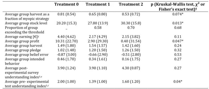
We found significant differences between treatments (Table 4). First, the threshold treatment 370
groups (T1, T2) cooperate more on average, participants use significantly less myopic strategies 371
and groups deplete significantly less the resource (higher average stock). Furthermore, the 372
groups playing in the threshold treatments which exceed the threshold, experience an important 373
cost that diminishes drastically their profit. We therefore observe a lower average in profit with 374
a high variability between groups. Furthermore, we observe an effect of uncertainty around the 375
threshold (T2). Groups who experience threshold uncertainty cooperate more if we consider the 376
14
ratio of harvest decision on the myopic strategy and the mean resource level. However, the 377
proportion of groups exceeding the threshold is higher than in the first treatment (T1)8.
378 379
Table 4: Comparison of proportions and averages across treatments.
380
Treatment 0 Treatment 1 Treatment 2 p (Kruskal-Wallis test, χ² or
Fisher’s exact test)ϯ
Average group harvest as a fraction of myopic strategy
0.81 (0.54) 0.65 (0.80) 0.53 (0.72) 0.074*
Average group stock level 20.20 (15.3) 27.80 (13.9) 30.30 (15.8) 0.013*
Proportion of group exceeding the threshold
_ 0.58 0.70 0.68
Average earning [€]χ 4.40 (4.62) 2.17 (4.29) 2.15 (3.82) 0.11
Average group profit 10.31 (22.70) 2.90 (29.30) 0.40 (31.54) 0.047*
Average group harvest 1.49 (1.80) 1.54 (1.57) 1.42 (1.60) 0.24
Average group pledge 1.02 (1.48) 1.20 (1.50) 1.26 (1.50) 0.32
Average group belief error -0.87 (3.00) -0.66 (2.90) -0.51 (2.80) 0.53
Average group intended behavior 0.46 (1.70) 0.34 (1.61) 0.16 (1.75) 0.27 Average post- experimental survey understanding index†,ν 3.90 (1.24) 3.90 (1.10) 4.30 (0.87) 0.27
Average pre- experimental test understanding index†,ґ
2.00 (1.00) 1.39 (1.00) 1.60 (1.20) 0.04*
Note: Standard errors in brackets.
*Indicates significance p<0.05, ** p<0.01 and *** p<0.001.
† Self-reported variable, obtained from pre and post-experimental survey (Appendix B).
Ϯ Kruskal-Wallis test is used to compare means across treatments and χ² or Fisher’s exact test (depending on the case frequencies) used to compare proportions across treatments.
χ Average earnings (from profits and belief elicitations) doesn’t include participation fees.
ν Average understanding index is the answer from the post-experimental survey on a five-point Likert scale.
Ґ Average pre- experimental test understanding index is the score from the 3 pre-experimental questions (Appendix B). A score of 3 indicates a perfect understanding, while a score of 0 a very weak comprehension of the experiment dynamic mechanisms before clarification by the experimenter.
381
The overall catch decreasing pattern until the steady state stock size corresponding to the 382
trigger strategy was found similar between groups in the treatment without a threshold (T0, 383
Figure 3). All groups in the treatment T0 followed the trigger strategy and exploited the resource 384
until the stationary non-cooperative equilibrium (10 units). Only 3 groups over 34 managed to 385
maintain the biomass level close to the long term optimal level (40 units), for which the 386
regeneration rate was the highest while the harvesting cost was low. They all belong to the 387
treatments groups (one in T1 and two in T2). 388
In contrast with our theoretical prediction, the majority of groups (7) in the certain thresholds 389
treatments (T1) harvest beyond the threshold. None of these groups is able to reverse the 390
negative trend of stock depletion despite the high penalty cost. We observe the same pattern in 391
the uncertain threshold treatment (T2) with 7 cases of exploitation falling beyond the threshold 392
8 We also test the potential effect of playing 2 games (phases) sequentially. We did not find any
significant difference between phases using the Mann-Whitney-Wilcoxon test on group averages (Appendix H).
15
level. Moreover, despite the high cost related to the full depletion of stocks, two groups have 393
intentionally exhausted the resource to end the experiment. 394
395
396
Figure 3: Time series of resource stock size (biomass in units) by treatments (T0, T1 and T2).
397
The grey dashed line corresponds to the threshold Blim in T1 and the shaded area to the
398
uncertainty range around the potential value of Blim in T2.
399 400
We observe a lower proportion of myopic strategies in the threshold treatments (T1 and T2) 401
which contradict the theoretical predictions (Figure 4). Moreover, we notice more cooperation 402
(lower proportion of myopic strategies) in the uncertain threshold treatment than in other 403
experimental conditions (Table 3). We also clearly discern a time pattern linked with the 404
scarcity of the resource regardless of the treatment. 405
16 407
Figure 4: Proportion of harvest as a fraction of myopic strategy over times by treatments (T0,
408
T1 and T2) summarized into a categorical variable: ‘Myopic’ if the ratio of the harvest choice 409
over the myopic strategy is superior or equal to 1 and ‘NonMyopic’ if the ratio is inferior to 1. 410
411
To go further into the analysis of individual strategies, we show that the more intensive harvest 412
pattern (Myopic behavior, Figure 5) in T0 during the first rounds (0 to 8) conduct the stock to Btr
413
(10 units) and zero profits as a result of the application of the trigger strategy. Participants’ 414
announcements (pledges) and harvest decisions are helpful to understand the start of the trigger 415
strategy (punishment of free-riders by overexploiting the stock until further depletion becomes 416
unprofitable). During the first rounds in which we observe the highest mean harvest decision, 417
participant’s pledges are strictly inferior to harvests conducting participants into intended free-418
riding behavior (intended behavior >0). On the other hand, mean participants’ beliefs are too 419
optimistic: they expect other players to harvest less following their announcements (belief error 420
<0). Threshold treatments exhibit the same pattern with a less marked trend in free-riding 421
intended behaviors and prediction of other participants’ harvests. The classification into distinct 422
subject types summarizes this information by showing the highest proportion of free-riders and 423
optimistic participants in the experiments (Figure 6). Likewise, this information highlights the 424
high frequency of consensual participant which strengthens the theoretical hypothesis that 425
participants use consensual punishment strategy. 426
17
Figure 5: Time series of mean harvest and pledge decisions, and mean resulting resource stock
428
size, profit, intended behavior and belief error by treatments (T0, T1 and T2). 429
18 431
Figure 6: Frequency of subject types for the whole experiments and by treatments (T0, T1 and
432
T2). Classification of subjects based on their highest frequency belief errors (optimistic: belief < 433
other harvest, realistic: belief = other harvest and pessimistic: belief > other harvest) and 434
intended harvest behaviors (free-rider: harvest > pledges / (N-1), consensual: harvest = pledges 435
/ (N-1) and altruistic: harvest < pledges / (N-1)). 436
3.2. Exploring predictors for cooperation
437
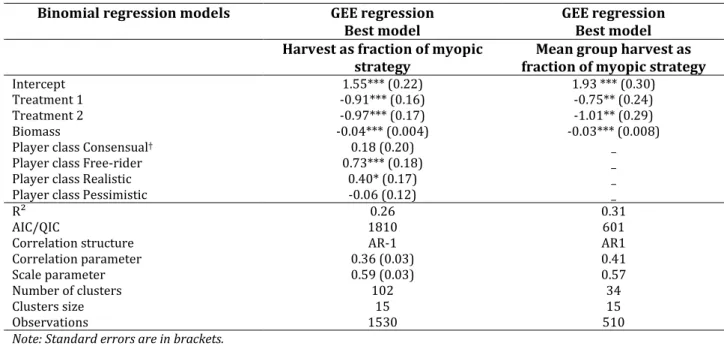
The selected GEE regression model (Table 5) 9 reveals that groups playing the threshold
438
treatment (T1 and T2, p < 0.001) are more cooperative. On average, the odds, ceteris paribus, of 439
behaving myopically in the no threshold treatment (T0) over the odds of behaving myopically in 440
the threshold treatments (T1 or T2) is about 2.56 (inverse of the odds in Table 5). In term of 441
percentage of variation, the odds of behaving myopically among the no threshold treatment 442
groups is around 156% higher than groups in the threshold treatment. The threat to cross the 443
threshold enhances cooperation by mitigating selfish behaviors. 444
We can also identify the effect of the resource scarcity on subjects mean harvest decisions. When 445
subjects start experiencing scarcity, they significantly tend to select myopic decisions (biomass 446
level effect, p<0.001). Participants are stuck in short-sighted competitive behaviors. In all 447
treatments, the proportion of myopic decisions increases by approximately a factor 3 to 4 448
between the first and the last rounds of the experiment (Figure 4). This observation is confirmed 449
by the average continuous decreasing trend of biomass throughout time (Figure 3). 450
The subject type is also an important explanatory variable which is defined by the ability of 451
participants during the experiment to predict other players’ behaviors (belief error) and their 452
intentions to follow or not the agreement contracted during the game (intended behavior, Table 453
9We also compared GEE models to random group effect generalized linear models (GLMM with package ‘lme4’ Bates et al., 2015 in R, Appendix I). The results are qualitatively similar with a higher magnitude of treatment and free-rider participant coefficients.
19
3). The presence of free-riding participants significantly affects the mean odds of choosing 454
myopic strategies. Those participants who deliberately deviate from the other pledges (catch > 455
pledge/2) selected on average more myopic strategies than other players and lead to stock 456
depletion with the implementation of the punishment (trigger) strategy. Furthermore, the 457
significant positive coefficient of realistic and consensual participants confirms our previous 458
analysis that participants use consensually a punishment strategy. 459
460
Table 5: Generalized Estimating Equation regression for the average probability of making a 461
myopic harvest decision. 462
Binomial regression models GEE regression
Best model
GEE regression Best model Harvest as fraction of myopic
strategy
Mean group harvest as fraction of myopic strategy
Intercept 1.55*** (0.22) 1.93 *** (0.30)
Treatment 1 -0.91*** (0.16) -0.75** (0.24)
Treatment 2 -0.97*** (0.17) -1.01** (0.29)
Biomass -0.04*** (0.004) -0.03*** (0.008)
Player class Consensual† 0.18 (0.20) _
Player class Free-rider 0.73*** (0.18) _
Player class Realistic 0.40* (0.17) _
Player class Pessimistic -0.06 (0.12) _
R² 0.26 0.31
AIC/QIC 1810 601
Correlation structure AR-1 AR1
Correlation parameter 0.36 (0.03) 0.41
Scale parameter 0.59 (0.03) 0.57
Number of clusters 102 34
Clusters size 15 15
Observations 1530 510
Note: Standard errors are in brackets.
*Indicates significance p<0.05, ** p<0.01 and *** p<0.001.
†Player classes are characterized by both belief errors and intended behavior (harvest decisions) to others pledge (Table 3): Optimistic; Pessimistic; Realistic and Consensual; Free rider; Altruistic.
4.
Discussion
463
The objective of this study was to experimentally investigate the effects that endogenously 464
driven, abrupt changes (i.e. tipping points) of the economic environment may produce on the 465
harvest and management decision of the EABFT (a CPR). We found that the existence of a latent 466
and endogenous economic shift significantly influenced resource decision maker strategies 467
regarding management cooperation and resource exploitation. Unlike our theoretical 468
predictions (Hypothesis 1), when the threat of a regime shift was present, we observed 469
relatively more cooperative behaviours and a more precautionary management of the 470
renewable resources. We also observed more cooperation when the position of the tipping point
471
is uncertain, rejecting our second hypothesis (Hypothesis 2). The threat of substantial losses 472
associated with the shift in economic conditions significantly increased the likelihood of 473
coordinating actions. 474
20
Our results about the influence of a tipping point on resource exploitation strengthen previous 475
observations by Schill et al. (2015) and Lindahl et al. (2016). They demonstrated that a certain 476
or a highly probable endogenous shift affecting the productivity of the resource creates the 477
condition to avoid a disaster such as a stock exhaustion. Similarly, avoiding an economic disaster 478
in a one-shot public good game with threshold is possible when it is in the interest of each 479
individual (disaster is severe enough) to coordinate and contribute accordingly (Barrett & 480
Dannenberg 2012; Barrett & Dannenberg 2013). But in contradiction with our theoretical 481
expectation, uncertainty around the position of the tipping point influences exploitation 482
strategies, enhancing instead of decreasing cooperation. Deviations from predictions in 483
uncertain decision problems are well known. From empirical evidence, we know that in complex 484
and uncertain decision problems (as used in our experiment), the assumptions underpinning the 485
expected utility theory are questionable (e.g., Tversky and Kahneman 1974). Decision makers 486
typically deviate from expected utility maximization and rely instead on heuristics (Moxnes, 487
1998 and Hey et al., 2009). Such theoretical biases bring insight to our experimental 488
observations which deviate from theoretical predictions and from previous static design results. 489
However, this result challenges previous findings obtained with one-shot public good games 490
under uncertain threshold, in which the uncertainty level around the position of the threshold 491
switches the game outcome from coordination to prisoner’s dilemma (Barrett & Dannenberg 492
2013). Observations have shown that participants decreasing their contribution under 493
uncertainty regime to an insufficient level would incur high economic loss and may not avoid the 494
disaster (e.g. cost due to climate change effects, in Barrett & Dannenberg, 2013). 495
By introducing complex resource dynamics and incomplete information conditions into the 496
experimental design, the focal point represented by the cooperative solution changes over time 497
and is path-dependent. The incentive to deviate from a past agreement increases throughout 498
time, as the probability of a game continuation decreases. Such conditions make cooperation and 499
coordination more unlikely. This has been demonstrated experimentally by Herr et al. (1997) 500
and Mason & Phillips (1997) when comparing static and dynamic designs. 501
Another interesting observation concerns the rare cases of groups (3 cases over 34) maintaining 502
the biomass level close to the long term optimal level (40 units) in our experiment. The 503
complexity and the high competitive feature of the experiment do not allow an agreement to 504
emerge efficiently with only the threat of using trigger strategy. Another explanation of the weak 505
cooperation level in our experiment could be related to the communication which has been 506
reduced to implicit communication through pledges in this experiment. An important factor 507
which has been excluded from our experiment is the introduction of face-to-face 508
communication. Previous CPR research works show that face-to-face communication is 509
important to determine whether groups will cooperate or not (e.g., Ostrom 2006). In complex 510
21
ecological dynamic experiments, Schill et al., (2015) and Lindahl et al. (2016) have shown that 511
the effectiveness of communication (group agreements), which underlies cooperation, can be 512
endogenous to the decision problem. The latent regime shift that people perceive as a threat in 513
their experiments seems to be the trigger of communication between subjects.
514
Finally, we found a clear trend of non-cooperative (myopic) strategies over time regardless of 515
the treatment. We found a strong correlation between non-cooperative strategies and the 516
scarcity of natural resources. Subjects are prone to competitive and more intensive fishing 517
behavior when the resource becomes scarcer. More surprisingly, the high cost of exceeding the 518
threshold does not affect this pattern. This result confirms previous findings by Osés-Eraso et al. 519
(2008). They had observed that users responded to scarcity with caution by observing directly
520
harvest levels but were, nevertheless, not able to avoid resource extinction. If we observed
521
directly the harvest instead of the ratio between harvest and the myopic harvest level, subjects
522
would have decreased their catch levels. But the latter do not represent a good indicator of the
523
cooperation level. When the situation becomes more competitive, with fewer natural resources
524
to share, participants’ behaviors seem to be driven by myopic strategies.
525
Our experiment is set in the context of the international management of a highly migratory fish, 526
the Atlantic Bluefin tuna (EABFT) fishery and reproduces a stylized representation of the 527
decision making process in the International Commission for the Conservation of Atlantic Tunas 528
(ICCAT), to the notable exception of communication exchanges between participants. Our results 529
confirm the possible change of management behaviours confronted to the threat of a shift in 530
economic conditions. This situation is somehow close to the context of trade ban in 2009 531
jeopardizing the future of the EABFT fishery, which has resulted in a dramatic decrease of 532
quotas (TACs) accepted by the fishing nations. When a critical threshold is introduced, decision 533
makers coordinate their efforts in order to avoid exceeding the potential threshold, becoming 534
more efficient, decreasing the rent dissipation and improving the sustainability of the resource. 535
We know from previous CPRs experiments the importance of direct communication in the 536
setting of cooperative agreements between participants (i.e Schill et al., 2015 and Lindahl et al., 537
2016). We leave to future works, the analysis of direct communications on cooperation in our 538
CPR dilemma. It is worthwhile noting that our results stem from laboratory experiments with 539
students as subjects. To increase confidence in our results, a next step would be to replicate this 540
design into the “battle field”, i.e. an international central institution such as the ICCAT 541
commission with actual policy makers. 542
5.
Acknowledgments
543
We are thankful for valuable comments received from Marc Willinger, Stefano Farolfi, Dimitri 544
Dubois, Nils Ferrand, Sander De Waard, members of the Laboratoire d’Economie Expérimentale 545
22
de Montpellier (LEEM) working group and members of the IM2E Experiments on Uncertainty 546
and Social Relations workshop. We thank Julien Lebranchu for his computer support, Dimitri 547
Dubois for his experiment assistance and Anne-Catherine Gandrillon for her language 548
corrections. We are also thankful for valuable comments received from two anonymous 549
reviewers. Finally, we acknowledge the financial support of the COSELMAR project (funded by 550
the Regional Council of Pays de la Loire) and from the University of Nantes and IFREMER for the 551
funding of a PhD. Last but not least, we would like to thank our experiment participants. 552
6.
References
553
Armsworth, P. R., and Roughgarden, J. E. 2003. The economic value of ecological stability. 554
Proceedings of the National Academy of Sciences, 100(12), 7147-7151. 555
Bailey, M., Sumaila, R. U., and Lindroos, M. 2010. Application of game theory to fisheries over 556
three decades. Fisheries Research, 102(1), 1-8. 557
Barrett, S. 2013. Climate treaties and approaching catastrophes. Journal of Environmental 558
Economics and Management, 66, 235-250. 559
Barrett, S., and Dannenberg, A. 2012. Climate negotiations under scientific uncertainty. 560
Proceedings of the National Academy of Sciences, 109(43), 17372-17376. 561
Bates D., Maechler M., Bolker, B., and Walker, S. 2015. Fitting Linear Mixed-Effects Models Using 562
lme4. Journal of Statistical Software, 67(1), 1-48 563
Biggs, R. and Blenckner, T. and Folke, C. and Gordon, L. and Norstrom, A. and Nystrom, M. and 564
Peterson, G. 2012. Regime shifts. In: Hastings A, Gross L (eds) Sourcebook in theoretical ecology. 565
University of California Press, Berkeley. 566
Boettiger, C., Bode, M., Sanchirico, J. N., LaRiviere, J., Hastings, A., and Armsworth, P. R. 2016. 567
Optimal management of a stochastically varying population when policy adjustment is costly. 568
Ecological Applications, 26(3), 808-817. 569
Brasão A., Duarte C.,C. and Cunha-E-Sá M. A. 2000. Managing the Northern Atlantic Bluefin Tuna 570
fisheries: the stability of the UN fish stock agreement solution. Marine Resource Economy, 15, 571
341-360. 572
Budescu, D., V., Rapoport, A. and Suleiman R. 1995. Common Pool Resource Dilemmas under 573
Uncertainty: Qualitative Tests of Equilibrium Solutions, Games and Economic Behavior, 10(1), 574
171-201. 575
Cullis-Suzuki, S. and Pauly, D. 2010. Failing the high seas: A global evaluation of regional fisheries 576
management organizations. Marine Policy, 34, 1036-1042. 577
Daw, T., and Gray, T. 2005. Fisheries science and sustainability in international policy: a study of 578
failure in the European Union’s Common Fisheries Policy. Marine Policy, 29(3), 189-197. 579
23
Fromentin, J. M., Bonhommeau, S., Arrizabalaga, H., and Kell, L. T. 2014. The spectre of 580
uncertainty in management of exploited fish stocks: The illustrative case of Atlantic bluefin tuna. 581
Marine Policy, 47, 8-14. 582
Fudenberg, D., and Tirole J. 1998. Game Theory. MIT Press, Cambridge, MA, USA. 583
Gordon, H., S. 1954.The economic theory of a common-property resource: the fishery. Palgrave 584
Macmillan, England, 178-203. 585
Hannesson, R. 1997. Fishing as a Supergame.Journal of Environmental Economics and 586
Management,32(3), 309-322. 587
Hannesson, R. 2011. Game Theory and Fisheries. Annual Review of Resource Economics, 3(1), 588
181-202. 589
Hardin, G. 1968. The tragedy of the commons. Science,162(3859), 1243-1248. 590
Hey, J. D., Neugebauer, T., and Sadrieh, A. 2009. An Experimental Analysis of Optimal Renewable 591
Resource Management: The Fishery. Environmental and Resource Economics, 44(2), 263-285. 592
Hilborn, R., Orensanz, J. M., and Parma, A. M. 2005. Institutions, incentives and the future of 593
fisheries.Philosophical Transactions: Biological Sciences, 47-57. 594
Hurry, G. D., Hayashi M. and Maguire, J. J. 2008. Report of the independent review. International 595
Commission for the Conservation of Atlantic Tunas (ICCAT), PLE-106/2008. Madrid, ICCAT. 596
http://www.iccat.int/Documents/Meetings/Docs/Comm/PLE-106-ENG.pdf (accessed February 597
17, 2017). 598
ICCAT. 2007. Report of the Standing Committee on Research and Statistics (SCRS). ICCAT Report 599
for the Biennial Period, 2006-2007, Part I (2006), Vol. 2.
600
http://iccat.int/Documents/BienRep/REP_EN_06-07_I_2.pdf (accessed January 21, 2017). 601
ICCAT. 2009. Report of the Standing Committee on Research and Statistics (SCRS). Report for the 602
Biennial Period, 2008-2009, Part I (2008), Vol 2.
603
http://iccat.int/Documents/BienRep/REP_EN_08-09_I_2.pdf (accessed January 14, 2017). 604
Juan-Jorda´, M. J., Mosqueira, I., Cooper, A. B., Freire, J. and Dulvy, N. K. 2011. Global population 605
trajectories of tunas and their relatives. Proceedings of the National Academy of Sciences, 108, 606
20650-20655. 607
Levhari, D., and Mirman, L. J. 1980. The great fish war: an example using a dynamic Cournot-608
Nash solution.The Bell Journal of Economics, 322-334. 609
Lindahl, T., Crépin, A. S., and Schill, C. 2016. Potential Disasters can Turn the Tragedy into 610
Success. Environmental and Resource Economics, 65(3), 657-676. 611
Maguire J. J., Sissenwine, M., Csirke, J., and Grainger, R. 2006. The state of world highly migratory, 612
straddling and other high seas fish stocks, and associated species. Fisheries Technical Papers, 613
495, FAO, Rome. 614
24
Maskin E., and Tirole J. 2001. Markov perfect equilibrium: I. Obervable actions. Journal of 615
Economic Theory, 100, 191-219. 616
McWhinnie S. F. 2009. The tragedy of the commons in international fisheries: an empirical 617
investigation. Journal of Environmental Economics and Management, 57, 312-333. 618
Milinski, M., Sommerfeld, R. D., Krambeck, H. J., Reed, F. A., and Marotzke, J. 2008. The collective-619
risk social dilemma and the prevention of simulated dangerous climate change. Proceedings of 620
the National Academy of Sciences, 105(7), 2291-2294. 621
Moxnes, E. 1998. Not Only the Tragedy of the Commons: Misperceptions of Bioeconomics. 622
Management Science, 44(9), 1234-1248. 623
Munro, G. R. 1979. The optimal management of transboundary renewable resources. Canadian 624
Journal of Economics, 12(3), 355-376. 625
Munro, G. R., Van Houtte, A., and Willmann, R. 2004. The conservation and management of 626
shared fish stocks: legal and economic aspects(Vol. 465). Food and Agriculture Organisation. 627
Osés-Eraso, N., Udina, F., and Viladrich-Grau, M. 2008. Environmental versus Human-Induced 628
Scarcity in the Commons: Do They Trigger the Same Response? Environmental and Resource 629
Economics, 40(4), 529-550. 630
Ostrom, E. 2006. The value-added of laboratory experiments for the study of institutions and 631
common-pool resources. Journal of Economic Behavior and Organization, 61(2), 149-163. 632
Patterson, K., and Résimont, M. 2007. Change and stability in landings: the responses of fisheries 633
to scientific advice and TACs. ICES Journal of Marine Science: Journal du Conseil, 64(4), 714-717. 634
Pauly, D., Christensen, V., Dalsgaard, J., Froese, R., and Torres, F. (1998). Fishing down marine 635
food webs. Science, 279(5352), 860-863. 636
Pintassilgo, P. 2003. A coalition approach to the management of high seas fisheries in the 637
presence of externalities. Natural Resource Modeling, 16(2), 175-197. 638
Pintassilgo, P., Finus, M., Lindroos, M., and Munro, G. 2010. Stability and success of regional 639
fisheries management organizations. Environmental and Resource Economics, 46(3), 377-402. 640
Pintassilgo, P., Kronbak, L. G., and Lindroos, M. 2015. International Fisheries Agreements: A 641
Game Theoretical Approach. Environmental and Resource Economics, 62(4), 689-709. 642
Scheffer, M., Westley, F., and Brock, W. 2003. Slow Response of Societies to New Problems: 643
Causes and Costs. Ecosystems, 6(5), 493-502. 644
Schill, C., Lindahl, T., and Crépin, A.S. 2015. Collective action and the risk of ecosystem regime 645
shifts: insights from a laboratory experiment. Ecology and Society, 20(1), 48. 646
Sumaila U.R. 2013. Game theory and fisheries. Essays on the tragedy of free for all fishing, 647
Routledge. 648
Teh, L., and Sumaila, U. 2015. Trends in global shared fisheries. Marine Ecology Progress Series, 649
530, 243-254. 650