General Formulation and Accurate Evaluation of Earth-Return Parameters for Overhead/Underground Cables

(1)

UNIVERSITÉ DE MONTRÉAL

GENERAL FORMULATION AND ACCURATE EVALUATION OF EARTH-RETURN PARAMETERS FOR OVERHEAD / UNDERGROUND CABLES

HAOYAN XUE

DÉPARTEMENT DE GÉNIE ÉLECTRIQUE ÉCOLE POLYTECHNIQUE DE MONTRÉAL

THÈSE PRÉSENTÉE EN VUE DE L’OBTENTION DU DIPLÔME DE PHILOSOPHIAE DOCTOR

(GÉNIE ÉLECTRIQUE) AOÛT 2018

(2)

ÉCOLE POLYTECHNIQUE DE MONTRÉAL

Cette thèse intitulée:

GENERAL FORMULATION AND ACCURATE EVALUATION OF EARTH-RETURN PARAMETERS FOR OVERHEAD / UNDERGROUND CABLES

présentée par : XUE Haoyan

en vue de l’obtention du diplôme de : Philosophiae Doctor a été dûment acceptée par le jury d’examen constitué de :

M. KOCAR Ilhan, Ph. D., président

M. MAHSEREDJIAN Jean, Ph. D., membre et directeur de recherche M. AMETANI Akihiro, Ph. D., membre et codirecteur de recherche M. SHESHYEKANI Keyhan, Ph. D., membre

(3)

DEDICATION

(4)

ACKNOWLEDGEMENTS

Foremost, I would like to express my very great appreciation to my Ph.D. supervisor Prof. Jean Mahseredjian for the continuous support of my research and the valuable study opportunity in Polytechnique Montréal.

I would like to express my sincere gratitude to my co-supervisor Prof. Akihiro Ametani for his patience, motivation and comprehensive knowledge. Advice given by him has been a great help in all the time of research.

Discussion and assistance provided by co-supervisor Prof. Ilhan Kocar were much appreciated. I would like to offer my special thanks to Prof. Piero Triverio and Mr. Utkarsh Patel for the comprehensive understanding of MoM-SO.

I would also like to thank Diane Desjardins and Gwendoline Le Bomin for their help in my French studies.

All colleagues at the department for their friendship and support. To those who already left: Isabel Lafaia, Baki Cetindag, Louis Filliot, Xiaopeng Fu, Fidji Diboune and Serigne Seye. To those who will continue: Anas Abusalah, Ming Cai, Jesus Morales, Miguel Martinez, Anton Stepanov, Aboutaleb Haddadi, Reza Hassani, Thomas Kauffmann, Masashi Natsui, David Tobar, Nazak Soleimanpour, Maryam Torabi, Amir Sadati and Willy Mimbe.

Finally, I would like to thank my family: my parents Feng Xue and Ming Wan, my wife Yanfei Liu for their support and encouragement.

(5)

RÉSUMÉ

La simulation de transitoire électromagnétique (EMT) dans les réseaux électriques est devenue un outil important pour la recherche et les applications pratiques. Les outils de simulation de type EMT nécessitent des modèles de ligne / câble aérien(ne) et de câble souterrain qui sont basés sur le calcul de paramètres d'impédance série et d'admittance shunt. Ces paramètres sont calculés en utilisant des données géométriques du système de transmission et des paramètres physiques. Un aspect important dans les calculs est la formulation de l'impédance et l'admittance de retour à la terre.

Premièrement, dans cette thèse, les formules nouvelles et généralisées d'impédance et d'admittance de retour à la terre sont dérivées pour une ligne aérienne et un câble souterrain, en se basant sur les équations de Maxwell avec des conditions initiales et aux limites complètes. De plus, les composantes complètes du champ électromagnétique émis sur la ligne aérienne et le câble souterrain sont dérivées. Afin d'éviter les difficultés numériques de la résolution complète, les formules d'impédance et d'admittance de retour à la terre sont simplifiées en adoptant les hypothèses appropriées. Ensuite, les formules approximées d'impédance et d'admittance de retour à la terre sont proposées pour le câble souterrain. Grâce à l'absence d'intégrale de Sommerfeld, les formules approximées peuvent être calculées facilement. Les formules existantes telles que les formules de retour à la terre par Pollaczek et Carson se déduisent simplement si les mêmes conditions sont adoptées dans la formulation généralisée proposée. Une Green fonction modifiée de retour à la terre de la méthode Method of Moment (MoM) - Surface Admittance Operator (SO) pour la ligne / le câble aérien(ne) est aussi dérivée. La stabilité numérique du MoM-SO pour la ligne / le câble aérien(ne) est améliorée en adoptant la Green fonction dérivée.

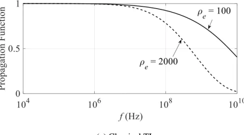
Ensuite, le concept de méthode de ligne de transmission (TL) étendue est proposé par rapport à la méthode de TL classique. En adoptant la méthode de TL étendue, l'allure des réponses en fréquence montrent des améliorations et des impacts significatifs dans les hautes fréquences pour une ligne aérienne, un câble aérien et un câble souterrain. Il est bien connu qu'il existe une transition de mode pour les lignes et les câbles aériens qui transforme l'onde de retour à la terre dans les fréquences basses en l'onde de surface dans les fréquences hautes. L'atténuation plus faible de l'onde de surface montre une différence significative pour les fonctions de propagation évaluées par la méthode de TL classique. Ensuite, les caractéristiques de l'onde de propagation du câble souterrain sont

(6)

évaluées par la méthode de TL étendue. L'influence des paramètres du sol, comme la résistivité et la permittivité de la terre, est clarifiée pour les caractéristiques de l'onde de propagation dans le domaine fréquentiel.

Suite à l'analyse du domaine fréquentiel, des simulations transitoires utilisant la méthode TL étendue sont effectuée aussi pour différentes applications aux réseaux électriques. Pour la première, le pic de tension du front d'onde de réponse à un échelon dans le domaine temporel est observé pour un bus simple à isolation gazeuse (GIB), car l'atténuation est plus faible dans les hautes fréquences. Ce phénomène explique que les tensions et courants transitoires mesurés dans les postes à isolation gazeuse (GIS) montrent des composantes fréquentielles qui sont entre quelques MHz et environ 100 MHz, et que les tensions et courants transitoires qui se trouvent le conduit du GIB sont maintenus pendant plus de quelques microsecondes. Ce phénomène ne peut pas être reproduit par la méthode TL classique. Ensuite, des études approfondies sont menées sur des transitoires très rapides (VFT) dans un 500 kV GIS en adoptant la méthode TL étendue. Les VFT simulations s'effectuent sur le modèle large bande (WB) de l'effet de dépendance en fréquence dans le Programme de Transitoire Électromagnétique (EMTP). Les effets de divers paramètres du GIS sur le VFT, par exemple la longueur et la mise à la terre du conduit, sont explorés. Ensuite, une analyse de la foudre sur une ligne aérienne de distribution est étudiée avec le résultat d'un essai pratique. Enfin, l'excitation des modes de propagations d'un câble avec transposition du blindage avec la méthode TL étendue montrent plus d’amortissement et une convergence plus lisse vers un régime permanent que la méthode TL classique. Les formules proposées sont aussi validées avec les résultats d'essais pratiques sur un 110 kV câble avec transposition du blindage.

(7)

ABSTRACT

Electromagnetic transient (EMT) simulations in power systems have become an important tool for both research and practical applications. EMT-type simulation tools require overhead line/cable and underground cable models which are based on the calculation of series impedance and shunt admittance parameters. These parameters are calculated using the input of transmission system geometrical data and physical parameters. An important aspect in the calculations is formulation of earth-return impedance and admittance.

As a first step in this thesis, new and generalized earth-return impedance and admittance formulas of overhead lines and underground cables are derived based on Maxwell equations with complete initial and boundary conditions. Also, the complete electromagnetic field components radiated by the overhead line and the underground cable are derived. In order to avoid numerical difficulties in the complete field solution, the earth-return impedance and admittance formulas are simplified by adopting the appropriate assumptions. Moreover, approximate earth-return impedance and admittance formulas for the underground cable are proposed. Those formulas can be easily calculated because no Sommerfeld integral is involved. In addition, existing formulas such as Pollaczek’s and Carson’s earth-return impedance formulas are easily deduced from the proposed generalized formulation under the conditions adopted by Pollaczek and Carson. A modified earth-return Green function of Method of Moment (MoM) - Surface Admittance Operator (SO) for overhead lines and cables is also derived. The numerical stability of MoM-SO for overhead lines and cables can be improved by adopting derived earth-return Green function.

Next, the concept of an extended transmission line (TL) approach is proposed in comparison with the classical TL approach. By adopting the extended TL approach, the characteristics of frequency responses of overhead lines, overhead cables and underground cables show significant improvements and impacts in high frequencies. As it is well-known, an overhead line and an overhead cable involve mode transition from a low frequency earth-return wave to a high frequency surface wave. The lower attenuation of the surface wave shows a significant difference in the propagation functions evaluated by the classical TL approach. Also, wave propagation characteristics of an underground cable are evaluated by the extended TL approach. The influences of earth parameters such as earth resistivity and permittivity are clarified for the wave propagation characteristics in frequency domain.

(8)

Further to the frequency domain analysis, transient simulations in time domain by adopting the extended TL approach are also performed for different power system applications. First of all, a spike-like voltage at the wave-front of a step response in time domain is observed for a simple gas-insulated bus (GIB) because of the lower attenuation in the high frequency region. This phenomenon explains the reason why measured transient voltages and currents in gas-insulated substations (GISs) show frequency components ranging from some MHz to about 100 MHz, and the transient voltages and currents along the GIB pipe are sustained for more than a few microseconds. This phenomenon cannot be reproduced by the classical TL approach. Then, this thesis performs thorough investigations of very fast transients (VFTs) in a 500 kV GIS by adopting the extended TL approach. VFT simulations are performed by the wide-band (WB) model of the frequency-dependent effect in the Electromagnetic Transients Program (EMTP). The effects of various GIS parameters such as length and pipe grounding on the VFTs are investigated. Also, a lightning surge analysis on an overhead distribution line is investigated together with a field test result. Finally, energization of propagation modes and a cross-bonded cable with the extended TL approach show more damping and smooth convergence to steady-state in comparison with the classical TL approach. The proposed formulas are also validated with a field test on a 110 kV cross-bonded cable.

(9)

LIST OF TABLES

Table 4.1: Summary of formulas adopted into extended and classical TL approaches ... 43

Table 4.2: Parameters of cables ... 61

Table 5.1: Effect of GIS length, Rg = 2 Ω ... 90

Table 5.2: The lowest natural frequency fn defined in (5.10) ... 92

Table 5.3: Effect of transformer stray capacitance, Rg = 2 Ω ... 93

Table 5.4: Effect of Rg, DS1 close, CB1 close, DS3 close, CB2 open ... 95

Table 5.5: Effect of Rg, DS1 close, CB1 close, DS2 close, CB2 open ... 96

Table 5.6: Effect of spacers for Case A1 and Case A2 ... 98

Table 5.7: Effect of DS3 length ... 100

Table 5.8: Effect of CB radius, CB radius: r1 = 12.5 cm, r2 = 64 cm and r3 = 66 cm ... 100

Table 5.9: Effect of source circuit parameters ... 101

Table 5.10: Operating DS and source conditions, all CBs close, DS2 close ... 104

(13)

LIST OF FIGURES

Figure 2.1: Configuration of an overhead line with N conductors above a homogenous earth ... 7

Figure 3.1: Configuration of an underground cable system with N cables buried in a homogenous earth ... 20

Figure 3.2: The integral path with the reference at the infinite depth ... 27

Figure 3.3: The integral path with the reference at the earth surface ... 29

Figure 4.1: A single overhead conductor, h1 = 10 m and r1 = 1 cm ... 44

Figure 4.2: Series impedance of the conductor illustrated in Figure 4.1 by the extended TL approach ... 45

Figure 4.3: Series impedance of the conductor illustrated in Figure 4.1 by the extended and classical TL approaches ... 46

Figure 4.4: Series impedance of the conductor illustrated in Figure 4.1 by the extended TL approach and MoM-SO, ρe = 100 Ωm and εr = 1 ... 47

Figure 4.5: Shunt admittance of the conductor illustrated in Figure 4.1 by the extended TL approaches ... 48

Figure 4.6: Shunt admittance of the conductor illustrated in Figure 4.1 by the extended and classical TL approaches ... 49

Figure 4.7: Attenuation constant of the conductor illustrated in Figure 4.1 by the extended TL approach ... 49

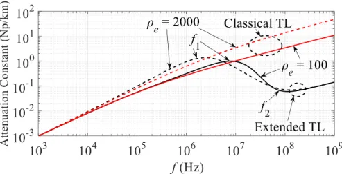
Figure 4.8: Attenuation constant of the conductor illustrated in Figure 4.1 by the extended and classical TL approaches, εr = 1 ... 50

Figure 4.9: Frequency responses of electromagnetic field components in the air, y = 0 m ... 53

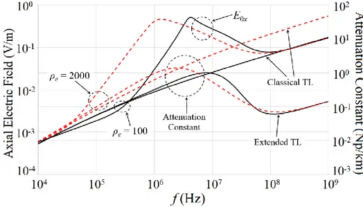
Figure 4.10: Frequency responses of attenuation constant and axial electric field component by the extended and classical TL approaches ... 54

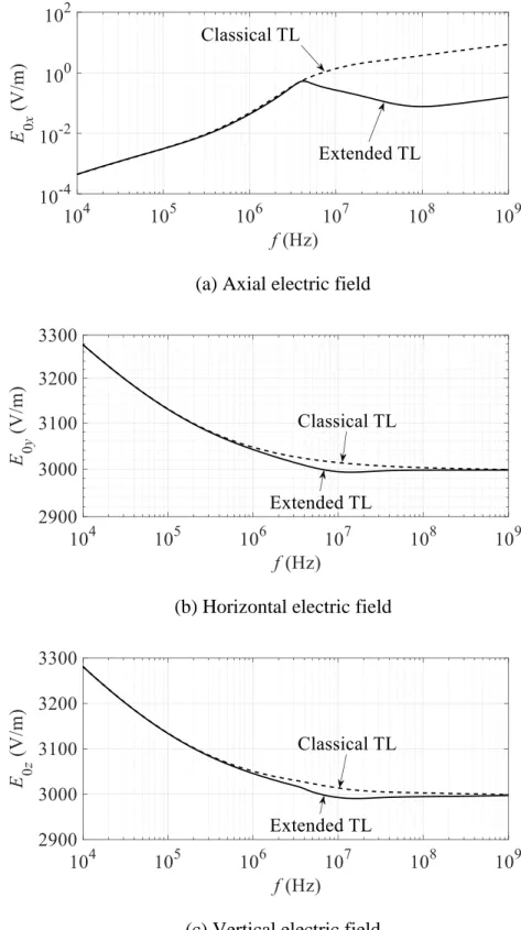
Figure 4.11: Comparison of electric field components at the conductor surface by the extended and classical TL approaches at z = 9.99 m and y = 0.01 m, ρe = 100 Ωm, εr = 1 ... 55

(14)

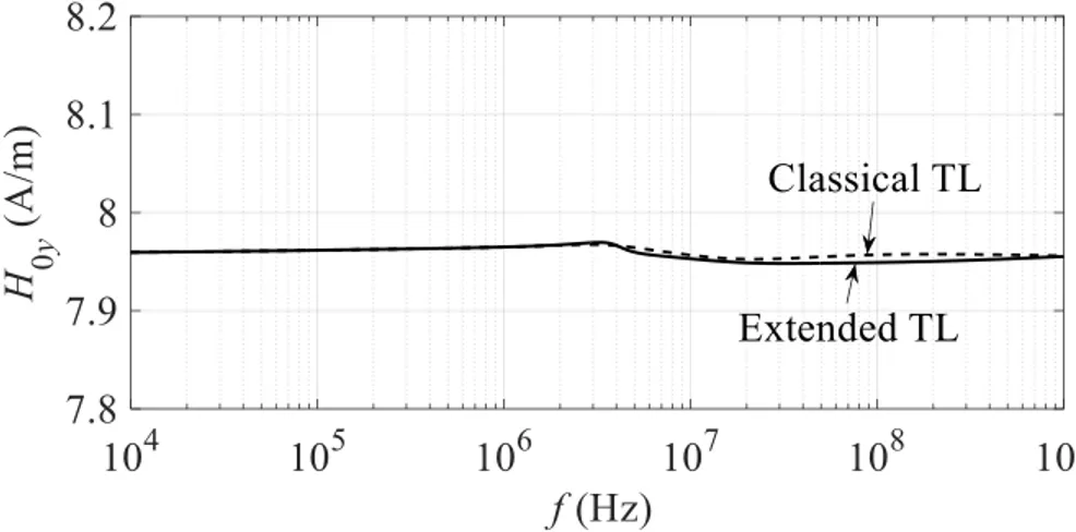
Figure 4.12: Comparison of horizontal magnetic field component by the extended and classical TL

approaches at z = 9.99 m and y = 0.01 m, ρe = 100 Ωm, εr = 1 ... 56

Figure 4.13: Cross-section of a 500 kV GIB, h1 = 2.45 m, r1 = 12.5 cm, r2 = 46 cm, r3 = 48 cm, ρc = 1.68×10-8 Ωm, ρp = 2.82×10-8 Ωm and SF6 gas εi = 1 ... 57

Figure 4.14: Modal attenuation constants of the GIB illustrated in Figure 4.13 by the extended and classical TL approaches, ρe = 100 Ωm and εr = 1 ... 58

Figure 4.15: Earth-return mode propagation function on the GIB illustrated in Figure 4.13 at distance x = 2 m from the sending end by the extended and classical TL approaches ... 59

Figure 4.16: Transition frequency f1 for the GIB illustrated in Figure 4.13 ... 60

Figure 4.17: Cross-section of a single core cable ... 60

Figure 4.18: Arrangement of three phase single core cable ... 61

Figure 4.19: Self-impedance of phase - a sheath by the extended TL approach ... 62

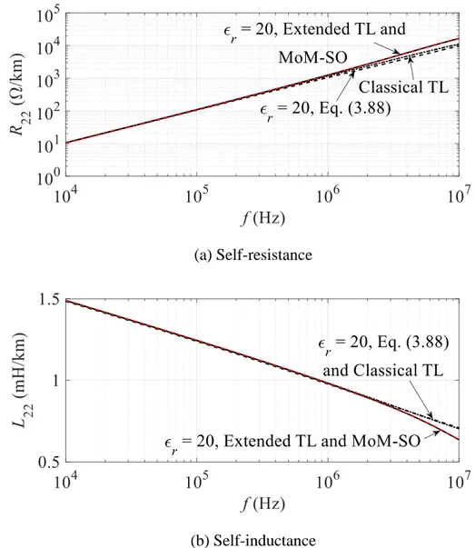
Figure 4.20: Self-impedance of phase - a sheath, ρe = 100 Ωm ... 63

Figure 4.21: Mutual impedance between phase - a and phase - b sheaths by the extended TL approach ... 64

Figure 4.22: Mutual impedance between phase - a and phase - b sheaths, ρe = 100 Ωm ... 65

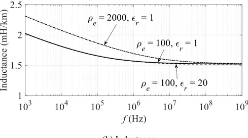
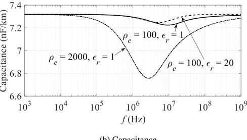
Figure 4.23: Self-admittance of phase - a sheath by the extended TL approach ... 66

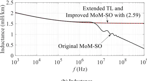
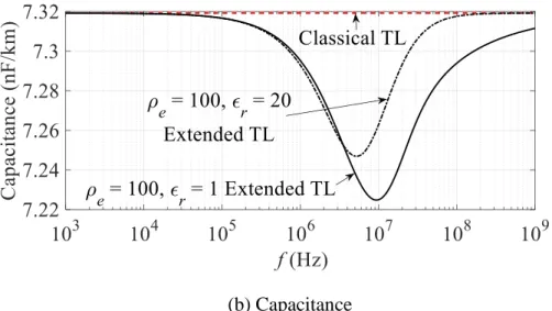
Figure 4.24: Self-admittance of phase - a sheath, ρe = 100 Ωm and εr = 1 ... 67

Figure 4.25: Mutual admittance between phase - a and phase - b sheaths by the extended TL approach ... 68

Figure 4.26: Mutual admittance between phase - a and phase - b sheaths, ρe = 100 Ωm and εr = 1 ... 69

Figure 4.27: Self-admittance of phase - a sheath, ρe = 100 Ωm and εr = 1 ... 70

Figure 4.28: Mutual admittance between phase - a and phase - b sheaths, ρe = 100 Ωm and εr = 1 ... 70

(15)

Figure 4.30: Self-admittance of phase - a sheath by the extended TL approach and (3.97) ... 72

Figure 4.31: Mutual admittance between phase - a and phase - b sheaths by the extended TL approach and (3.97) ... 73

Figure 4.32: Modal propagation constants on Cable 1 in Figure 4.18 by the extended and classical TL approaches, ρe = 100 Ωm and εr = 1 ... 74

Figure 5.1: Step response on the core of GIB in Figure 4.13 by the extended and classical TL approaches at x = 12 m, εr = 1 ... 80

Figure 5.2: Step response on the core of GIB in Figure 4.13 by the extended and classical TL approaches at x = 2 m and 12 m, ρe = 100 Ωm and εr = 1 ... 81

Figure 5.3: Simulation circuit for a 500 kV cascaded GIB, Rg1 = Rg2 = 2 Ω, ρe = 100 Ωm, εr = 1, x1 = 2 m and x2 = 10 m ... 81

Figure 5.4: Core voltage V2c at the open-circuited end ... 82

Figure 5.5: Transient current I2p through grounding resistance Rg2 = 2 Ω at the pipe receiving end ... 83

Figure 5.6: Frequency spectra of the voltage in Figure 5.4 and current in Figure 5.5 ... 85

Figure 5.7: Layout of a 500 kV GIS ... 87

Figure 5.8: Single-phase expression (core circuit) of the 500 kV GIS in Figure 5.7 ... 87

Figure 5.9: Core voltage at node N1 ... 88

Figure 5.10: Pipe voltage at node N1 by the extended TL approach ... 89

Figure 5.11: Frequency spectra of core and pipe voltages at node N1 ... 90

Figure 5.12: Core voltage at node N1 for Case A1 to Case A3 ... 91

(16)

Figure 5.14: Core voltage at node N1 for Case A5 ... 94

Figure 5.15: Frequency spectra of core voltages at node N1 for Case A4 and Case A5 ... 95

Figure 5.16: Core voltages at node N1 for Case B11 and Case B12 ... 96

Figure 5.17: Frequency spectra of core voltages at node N1 for Case B11 and Case B12 ... 97

Figure 5.18: Voltage distribution for Case B11 to Case B14 ... 97

Figure 5.19: Frequency spectra of core voltages at node N1 for Case C11 and Case C12 ... 98

Figure 5.20: Core voltage at node N1 for Case D3 ... 100

Figure 5.21: Frequency spectra of core voltages at node N1 for Case D3 and Case D4 ... 101

Figure 5.22: Core voltages at node N1 for Case E2 and Case E3 ... 102

Figure 5.23: Frequency spectra of core voltages at node N1 for Case E2 and Case E3 ... 103

Figure 5.24: Core voltages at node N1 for Case F1 to Case F3 ... 105

Figure 5.25: Frequency spectrum of core voltage at node N1 for Case F3 ... 105

Figure 5.26: Maximum voltage distribution for Case F1 to Case F3 ... 106

Figure 5.27: Maximum voltage distribution for Case G1 to Case G3 ... 107

Figure 5.28: Lumped-parameter equivalent circuit of a GIS ... 108

Figure 5.29: A 6.6 kV three phase overhead distribution line, h1 = 10 m, h2 = 11 m, d12 = d23 =1 m, rp = 0.437 cm, rg = 0.26 cm, ρp = ρg = 1.68×10-8 Ωm, ρe = 100 Ωm and εr = 1 ... 110

Figure 5.30: Model circuit for a step current simulation ... 111

Figure 5.31: Step surge voltages and currents at Node1 ... 112

Figure 5.32: Test circuit of lightning and its path to house, Fo: flashover between the pole and transformer neutral wire ... 112

Figure 5.33: Comparison of lightning surge by test and simulation results ... 113

Figure 5.34 Simulation circuits for energization of modes with cable length x ... 114

Figure 5.35: Phase - a core voltage at the receiving end for coaxial mode energization with x = 263 m ... 114

(17)

Figure 5.36: Phase - b sheath voltage at the receiving end for inter-sheath mode energization with

x = 263 m ... 115

Figure 5.37: Phase - b sheath voltage at the receiving end for inter-sheath mode energization with ρe = 100 Ωm, εr = 1 and x = 1 km ... 116

Figure 5.38: Sheath voltages at the receiving end for earth-return mode energization with ρe = 100 Ωm and x = 263 m ... 117

Figure 5.39: Single point bonding (two sections) with ECC and SVL [5] ... 119

Figure 5.40: Cross bonding without core transposition, a major section [5] ... 120

Figure 5.41: Cross bonding with core transposition, a major section [5] ... 121

Figure 5.42: Cross bonding without core transposition, a major section with link box and SVLs [5] ... 121

Figure 5.43: Link box with cross bonding connection and SVLs [96] ... 122

Figure 5.44: Test circuit for Cable 2 with a major section shown in Figure 5.40, ρe = 100 Ωm and εr = 1 ... 122

Figure 5.45: Field test results on the cable in Figure 5.44 ... 123

Figure 5.46: EMTP simulation results on the cable in Figure 5.44 ... 125

Figure 5.47: Core and sheath voltages at the receiving end of the cross-bonded cable in Figure 5.44, ρe = 100 Ωm and εr = 1 ... 126

Figure 5.48: Sheath voltage at the receiving end of the cross-bonded cable in Figure 4.18 (a), ρe = 100 Ωm and εr = 1 ... 126

(18)

LIST OF SYMBOLS AND ABBREVIATIONS

A Voltage transformation matrix

α Attenuation constant

B Current transformation matrix

β Phase constant

c Phase velocity

CB Circuit breaker

CP Constant parameter

DS Disconnector

ECC Earth continuity cable EMT Electromagnetic transient EMI Electromagnetic interference

EMTP Electromagnetic transients programs

F Vector field

FEM Finite element method

FW Fast wave

GIB Gas-insulated bus GIS Gas-insulated substation LCP Line / cable parameters MoM Method of moment

NLT Numerical Laplace transform

Pe Earth-return potential coefficient matrix based on quasi-TEM assumption

SA Surface attach

(19)

SVL Surge voltage limiter TE Transverse electric

TEM Transverse electromagnetic

TL Transmission line

TM Transverse magnetic

VFT Very fast transient

WB Wide-band

Ye Earth-return admittance matrix based on complete field solution

Ze Earth-return impedance matrix based on complete field solution

Ze Earth-return impedance matrix based on quasi-TEM assumption

(20)

LIST OF APPENDICES

Appendix A - Expressions of Sommerfeld integrals ... 145 Appendix B - List of publications ... 150

(21)

CHAPTER 1 INTRODUCTION

1.1 Motivation

The Electromagnetic Transients Program (EMTP) [1], [2] has been widely accepted and used all over the world as a standard and powerful simulation tool for studies and research on power system issues. The studies of electromagnetic transients are the most difficult and complicated ones. Because the EMT-type simulation tool is based on circuit theories, it requires the circuit parameters to perform simulations. Among various parameters, the series impedance and shunt admittance play an important role in the steady-state and transient phenomena on an overhead line, an overhead cable and an underground cable.

The generalized impedance and admittance formulas were found in [3]-[5] (Ametani) and implemented into the EMTP subroutine called Cable Constants in 1976. The Cable Constants are still widely used to calculate the parameters of overhead lines and underground cables in EMTP [1], [2].

In the documented formulas [3], the return parameters are important. The derivation of earth-return impedance formulas for an overhead line started in 1920 [6], [7] (Carson and Pollaczek formulas). Although their approaches involved some inaccurate initial assumptions of fields [8], their formulas have been used since 1930. Because of the publications of Carson and Pollaczek, a number of different and improved methods have been developed, but some adopted Carson’s and Pollaczek’s initial assumptions, and are regarded as Carson’s or Pollaczek’s corrections [9]-[16]. In [17], [18] (Wise) modified the uniform current and field assumptions [8] from Carson and Pollaczek, and more generalized earth-return impedance and admittance of an overhead line above a homogenous earth were introduced. The homogenous earth model was further improved by [19]-[21] (Nakagawa), [22] (Ametani) and recently by [23], [24], (Papadopoulos) who also extended the formulas of earth-return impedance and admittance for the earth configurations consisting of several horizontal layers with different electromagnetic characteristics. The calculated results and performances of different electromagnetic characteristics of earth were discussed by [25]-[27]. The aforementioned methods only considered the axial electric field in the formulations. An attempt to find exact solutions of the problem was proposed by [28], [29] (Kikuchi). In [30]-[32]

(22)

(Wait) extended Kikuchi’s work by adopting the method of complete Hertzian vector. Other attempts of complete field solutions of an overhead line were found by [8] (Olsen) and [33], [34] (Bridges) with the same method of [30]-[32]. In [35]-[39], it proposed different approaches in which the formulation of earth-return impedance and admittance are based on the vertical electric field and voltage propagation equation.

Propagation characteristics of an overhead line were also investigated and discussed in [28], [29]. In [28], [29], it pointed out that the wave propagation along an overhead line showed a transition between quasi-transverse electromagnetic (TEM) mode and transverse magnetic (TM) or transverse electric (TE) surface wave mode in a high frequency, and it was named Sommerfeld-Goubau propagation [28], [29]. For a clarity of definition, it has [28], [29]:

 TEM mode: neither electric nor magnetic field in the direction of wave propagation.  TE mode: no electric field in the direction of wave propagation.

 TM mode: no magnetic field in the direction of wave propagation.

Recently, in [26], it further discussed the effect of earth-return admittance of overhead lines. A more general propagation characteristic was proposed by [40], [41] (Olsen) and [42] (Kuester) for investigations of a full frequency spectrum propagation of an overhead line. In general, the totally excited current on a conductor due to a finite source consists of a sum of discrete propagation modes or guided wave modes as well as a contribution from continuous propagation modes or radiation modes. Two different discrete roots can be extracted from the evaluation of a complete form of the propagation constant by Newton-Raphson’s method [37]. One of the roots represents the transmission line (TL) mode, and it is associated with quasi-TEM mode. The TL mode reduces to the pure TEM mode of a conductor over a perfectly conducting earth. Another one is named fast wave (FW) mode or surface attached (SA) mode which is supported by the air-earth interface and can be related to the Zenneck surface wave. It should be noted that the TL mode is characterized by a smaller attenuation constant than the FW mode in a high frequency.

In [7] (Pollaczek), a formula of the earth-return impedance for an underground cable is also developed. The extended expression of Pollaczek’s formula is proposed in [9], [14]-[16], [43]-[46]. Some simplified closed-form approximation for the formulas in [7] and [43] are made and

(23)

summarized in [47]-[50]. Also, references [51]-[53] tried to revise the numerical instability by adopting different numerical methods.

In [54], [55] (Wait) and [56], [57] (Bridges) derived the complete field solutions of an underground cable which buried in a homogenous earth. The formulas of the earth-return impedance and admittance were deduced from the axial electric field with the impedance boundary condition at the outer radius of cable. Recently, lightning induced voltages are studied on an underground cable [58] by adopting the formulas based on reference [44]. Also, another quasi-TEM based earth-return admittance formula is derived in [59], [60], however the formula relies on the earth surface as the reference of the line voltage integral [59], [60].

It is crucial to recognize that a thin wire approximation is made for all the above methods. This assumption means that the carried current of a conductor is assumed to be only the axial direction of waveguide and uniformly distributed around the circumference of the conductor. Under this approximation, the current can be regarded as a filamentary current and located at the center of the conductor [61].

Except the analytical methods discussed above, the numerical electromagnetic analysis [62]-[70] is another approach for the calculations of parameters of lines and cables.

This thesis emphasizes the derivation of new and generalized earth-return impedance and admittance formulas of an overhead line, an overhead cable and an underground cable. The derived analytical formulas and Method of Moment (MoM) - Surface Admittance Operator (SA) method [64]-[67] are compared to each other. Also, the frequency and transient responses of different power system applications by adopting the newly derived formulas are investigated.

1.2 Thesis outline

This thesis is composed of six chapters and two appendices.  CHAPTER 1 INTRODUCTION

This chapter introduces the motivation of this Ph.D. work, highlights its contributions, publications and summarizes the contents of each chapter.

 CHAPTER 2 DERIVATION OF ELECTROMAGNETIC FIELD EQUATIONS AND EARTH-RETURN PARAMETERS FOR AN OVERHEAD LINE

(24)

The essential formulations of electromagnetic field components and the earth-return impedance and admittance of an overhead line with N conductors are proposed and derived in this chapter. The discussion of existing formulas is also included. A modified earth-return Green function is derived to eliminate the numerical instability of MoM-SO for an overhead line and cable.

 CHAPTER 3 DERIVATION OF ELECTROMAGNETIC FIELD EQUATIONS AND EARTH-RETURN PARAMETERS FOR AN UNDERGROUND CABLE

It presents the essential formulations of electromagnetic field components and the earth-return impedance and admittance of a multi-phase underground cable. It shows approximate earth-return impedance and admittance formulas. Also, the drawbacks of existing formulas are made clear in comparison with the derived complete formulas.

 CHAPTER 4 WAVE PROPAGATION IN FREQUENCY DOMAIN

This chapter explains the details of extended TL and classical TL approaches. It contains the calculations of wave propagation characteristics in frequency domain for an overhead line, an overhead cable and an underground cable.

 CHAPTER 5 TRANSIENT SIMULATIONS IN TIME DOMAIN

The transient simulations in time domain of different power system applications by adopting the extended and classical TL approaches presented in Chapter 4 are studied and investigated.

 CHAPTER 6 CONCLUSIONS

It presents the main conclusions of this thesis and future works.  APPENDIX A

It summarizes Sommerfeld integrals used in Chapter 2 and Chapter 3.  APPENDIX B

It shows the list of publications.

1.3 Contributions

(25)

 Derivation of new and generalized earth-return impedance / admittance formulas for an underground cable

New and generalized formulas of the earth-return impedance and admittance on an underground cable based on the complete field solution are derived. Differences of wave propagation and surge characteristics calculated by the newly proposed formulas and existing formulas implemented in EMTP are investigated. It is made clear that the complete formulas of impedance and admittance should be adopted especially when studying high-frequency phenomena. Also, the proposed impedance formula is verified in comparison with computed results by MoM-SO method.

 Time responses of an overhead cable due to mode transition from TEM to TM or TE propagation

It is known that wave propagation on an overhead conductor shows mode transition from a TEM mode at low frequencies to TM or TE modes at higher frequencies and finally reaches the so-called Sommerfeld-Goubau (surface wave) propagation with lower attenuation than that of the TEM mode [26], [28], [29]. The lower attenuation is estimated to influence significantly transient responses in time domain. However, all the previous studies were carried out in frequency domain. Thus, the basic characteristics of time domain responses considering mode transition which have not been studied in the past are investigated. The step response and switching surges of an overhead cable are calculated by using numerical Laplace transform (NLT) [71]-[73] and wide-band (WB) model in EMTP [1], [74].

 Mode transition of an overhead conductor from the viewpoint of the axial electric field This work investigates the frequency responses of electric and magnetic fields by deriving the formulas based on the complete field solutions in comparison with the formulas derived using the Carson or Pollaczek’s approach [6], [7]. Specifically, the correlation between the axial electric field and the attenuation constant is confirmed and validated in the mode transition area.

 Electromagnetic disturbances in gas-insulated substation (GIS) and very fast transient (VFT) calculations

VFTs are produced in a GIS during switching operation of a disconnector (DS) or a circuit breaker (CB) [75]-[77]. Because of very high frequency components, the VFTs in the GISs can cause electromagnetic interference (EMI) such as malfunctions in control circuits of the GISs [78]-[84].

(26)

In this work, modelling of GIS elements by the extended TL approach is explained. Also, the sensitive analysis of GIS parameters in VFT calculations are investigated.

 New cable parameters code

The newly produced cable parameters code can deal with the series impedance and shunt admittance for overhead cables, underground cables and overhead-underground cables above or buried in up to five layers of stratified earth.

Equation Chapter (Next) Section 1 Equation Section (Next)

(27)

CHAPTER 2 DERIVATION OF ELECTROMAGNETIC FIELD

EQUATIONS AND EARTH-RETURN PARAMETERS FOR AN

OVERHEAD LINE

In this chapter, formulas of the complete electromagnetic field solutions on an overhead line with N conductors are derived based on rigorous Maxwell equations. The derived formulas of electromagnetic fields are applied to formulate a generalized earth-return impedance and admittance on the multi-phase overhead line. Existing formulas of the earth-return impedance and admittance are discussed in comparison with the derived formulas. Finally, a modified earth-return Green function is derived and it is used for the recently developed software called MoM-SO [64]-[67]. By adopting the newly derived Green function, MoM-SO becomes able to generate accurate parameters of overhead lines within TEM mode of wave propagation, and the numerical instability observed in the original MoM-SO is eliminated [66], [67].

2.1 Derivation of electromagnetic field formulas

An overhead line with N conductors is located above a homogenous earth, as illustrated in Figure 2.1.

Figure 2.1: Configuration of an overhead line with N conductors above a homogenous earth The air is the medium in the region z  , and characterized by permeability 0  and permittivity₀

0

 . The region of z  is the lossy earth, and it is characterized by permeability 0  , permittivity ₁

y

x

z

Earth μ1, ε1,σ1 Air μ₀,ε₀ Conductor - m

. . .

Im dm dn hn hm Conductor - n In

(28)

1

 and conductivity  . It is assumed that the radius of each conductor is small compared with the ₁ height and separation. Thus, a filament current approximation can be adopted where all the conductor currents are only expressed by the axial component [35].

There exists as many propagation modes as the number of conductors in the system [35]. The conductor - m with radius r_mcarries the following current in phase domain [38].

 

1 N m mv v v I x B i x  



(2.1)

where B_mv is the mv-th element of the N N unknown current transformation matrix B (to be determined by impedance boundary condition) and the v-th modal current i_v

 

x is defined by:

 

jk xv

v vp

i x i e (2.2)

where i is the amplitude of the modal current and _vp kv is the unknown wave number of the v-th mode.

The electromagnetic vector fields can be defined by using Hertz vectors as [85]:

2 _j      E E  M E Π Π Π (2.3) 2 j      M M  E H Π Π Π (2.4)

where  is angular frequency.

E

Π and ΠM are electric and magnetic Hertz vectors. It should be noted that any continuously

differentiable vector field is define by:

x y z

F F F

 _x  _y  _z

F e e e (2.5)

where e_x, e and _y ez be the corresponding basis of unit vector e.

For the present problem, it is convenient to adopt only x-component of Hertz vectors because ΠE

(29)

Thus, the expressions of the x-component of the electric and magnetic Hertz vectors at any point in the air (“0”) and earth (“1”) can be derived as a sum of contributions by the current in each conductor [38]. By adopting the superposition theorem, it gives:









0 0 1 , , , , N E Em m x y z x y z   



 (2.6)









0 0 1 , , , , N M Mm m x y z x y z   



 (2.7)









1 1 1 , , , , N E Em m x y z x y z   



 (2.8)









1 1 1 , , , , N M Mm m x y z x y z   



 (2.9)

where ₀_Em



x y z, ,



, ₀_Mm



x y z, ,



, ₁_Em



x y z, ,



and ₁_Mm



x y z, ,



are the x-components of electric and magnetic Hertz vectors in the air and earth, generated by the current I_m

 

x of the m-th cable.

By adopting the formulas of Hertz vectors [30] into (2.6) to (2.9), the following formulas are deduced.





 

0   0   0 0 2 0 1 1 , , 4 m v m v m z h u z h u N N j y d Ev E mv v v m v a j e R e x y z B i x e d u k   _       _ _       





(2.10)





0

 

  0   0 ₂ 0 1 1 , , 4 m v m z h u N N j y d Mv M mv v v m v a j R e x y z B i x e d u k   _     _ _      





(2.11)





 

1 0   0 1 2 0 1 1 , , 4 v m v m zu h u N N j y d Ev E mv v v m v a j T e x y z B i x e d u k   _    _ _      



_

(2.12)





 

1 0   0 1 ₂ 0 1 1 , , 4 v m v m zu h u N N j y d Mv M mv v v m v a j T e x y z B i x e d u k   _    _ _      





(2.13)

(30)

2 2 2 0v v a u   k k , u_1v  2k_v2k_e2 (2.14) with 2 0 0 a k  j j , k_e2 j ₁



₁ j₁



(2.15) The irrationals R_Ev, R_Mv, T_Ev and T_Mv are derived by adopting the following boundary conditions [30] at the air / earth interface (z  ), referred to the v-th mode. 0

0 1 0 1 0 1 0 1 x x y y x x y y E E E E H H H H     _   _   _ (2.16)

where E_x, E , _y Hx and H are axial and horizontal electric and magnetic field components. y Substituting (2.10) to (2.13) into (2.16) and assuming ₁ ₀, R_Ev and R_Mv can be deduced.

2 2 0 2 2 2 2 0 1 0 1 1 1 2 a v v Ev v v a v e v a v k u k R u u k k k u k u      __  __   _  _ (2.17)





2 2 2 2 2 2 0 1 0 1 0 1 2 a v a Mv v v e v a v a v k k k R u u k u k u j k k       _  _    _ _ (2.18)

By adopting (2.17) and (2.18) into (2.10) and (2.11), and solving (2.3) and (2.4), the formulas of electromagnetic field components at an arbitrary point in the air are derived.









 

0 0 1 1 , , , , , , N N x x m m mv v m v E x y z y z d h v B i x   



 (2.19)









 

0 0 1 1 , , , , , , N N y y m m mv v m v E x y z y z d h v B i x   



 (2.20)









 

0 0 1 1 , , , , , , N N z z m m mv v m v E x y z y z d h v B i x   



 (2.21)









 

0 0 1 1 , , , , , , N N x x m m mv v m v H x y z y z d h v B i x   



 (2.22)

(31)









 

0 0 1 1 , , , , , , N N y y m m mv v m v H x y z y z d h v B i x   



 (2.23)









 

0 0 1 1 , , , , , , N N z z m m mv v m v H x y z y z d h v B i x   



 (2.24)

where E_z



x y z and , ,



H_z



x y z are vertical electric and magnetic field components. The kernel , ,



functions ₀_x



y z d, , _m,h v_m,



, ₀_y



y z d, , _m,h v_m,



, ₀_z



y z d, , _m,h v_m,



, ₀_x



y z d, , _m,h v_m,



,





0y y z d, , m,h vm,

 and ₀_z



y z d, , _m,h v_m,



are given in Appendix A.1.

Equations (2.19) to (2.24) can be rewritten into matrix expressions as a function of the exciting modal currents.





































 

0 0 0 1 0 0 0 0 0 0 , , , , , ,1 , , , , , , , , , ,1 , , , , , , , , , ,1 , , , , x x m m x m m y y m m y m m N z z m m z m m E x y z y z d h y z d h N i x E x y z y z d h y z d h N i x E x y z y z d h y z d h N     _ _ _ _     _ _  _  _   _ _     _ _ __ __     (2.25)





































 

0 0 0 1 0 0 0 0 0 0 , , , , , ,1 , , , , , , , , , ,1 , , , , , , , , , ,1 , , , , x x m m x m m y y m m y m m N z z m m z m m H x y z y z d h y z d h N i x H x y z y z d h y z d h N i x H x y z y z d h y z d h N     _ _ _ _     _ _  _  _   _ _     _ _ __ __     (2.26) where









0 0 1 , , , , , , , , N x m m x m m mv m y z d h v y z d h v B   



 (2.27)









0 0 1 , , , , , , , , N y m m y m m mv m y z d h v y z d h v B   



 (2.28)









0 0 1 , , , , , , , , N z m m z m m mv m y z d h v y z d h v B   



 (2.29)









0 0 1 , , , , , , , , N x m m x m m mv m y z d h v y z d h v B   



 (2.30)









0 0 1 , , , , , , , , N y m m y m m mv m y z d h v y z d h v B   



 (2.31)

(32)









0 0 1 , , , , , , , , N z m m z m m mv m y z d h v y z d h v B   



 (2.32)

The matrices expressions (2.25) and (2.26) describing the electromagnetic field components can be also represented in the following compact forms.

0 0 0 0     _ E Φ i H  i (2.33)

where E₀ and H₀ are N  electromagnetic field vectors, 1 Φ₀ and ₀ are 3 N modal current to field operator’s matrices, and i is an N  modal current vector. 1

It should be noted that (2.33) derived in the above is based on the assumption of unidirectional propagation of voltage and current waves. The responses of electromagnetic fields should be related to the exciting sources which are impressed by the transmitting device. Thus, the transfer function from voltage to field can be defined by using Φ₀ and ₀ matrices together with the following modal current vector [4], [5]:

1 1

0

 -

-f

i B Y AζA V (2.34)

where Y₀ is an N N characteristic admittance matrix of an overhead line in phase domain, A is an N N voltage transformation matrix, ζ is an N N reflection free transition diagonal matrix,

f

V is an N  impressed voltage source vector, and 1

 

_T -1 A = B (2.35)





diag _ejk xv  ζ (2.36)

Equation (2.33) can be rewritten by replacing i by (2.34):

1 1 0 0 0 1 1 0 0 0   _   _ - -f - -f E Φ B Y AζA V H  B Y AζA V (2.37)

Therefore, the radiated electromagnetic fields of a multi-phase overhead line can be calculated by applying the impressed voltage source V_f in (2.37).

(33)

2.2 Derivation of generalized earth-return impedance and

admittance formulas

In this section, the generalized earth-return impedance and admittance formulas are derived based on the electromagnetic field components in Section 2.1. Then, the derived formulas are discussed in comparison with existing formulas.

2.2.1 Complete field solution

The same configuration of an overhead line with N conductors illustrated in Figure 2.1 is considered. The continuity of axial electric field must be fulfilled at the air / conductor interface for each conductor in the configuration. The x-component of electric field along the n-th overhead conductor can be expressed by:

 





 

1 , N xn sn n nv v v E x Z r v B i x  



: n 1, ,N (2.38) where r_n is the radius of the n-th conductor, B_nv is the nv-th element of B , and Z_sn



r v is the _n,



surface impedance of the n-th conductor for the v-th mode [3].

By adopting the impedance boundary condition into (2.19) and (2.38), the continuity gives





 

0





 

1 1 1 , , , , , N N N sn n nv v x n n m m mv v v m v Z r v B i x d h d h v B i x     





(2.39)

In the evaluation of the right side of (2.39), the self-element, nm, is calculated at the surface of conductor. The mutual element, n , can be calculated at the center of two conductors. Whenm

1

N  , (2.39) becomes the same as the exact approach in reference [31].

Equation (2.39) can be rewritten in the following matrix expression based on an eigenvalue analysis [4]. 2 v k  r v v P B = B (2.40)

where vector B_v is related to the v-th column of B and N N matrix Pr is defined by:

 

-1

2 1



r r r

(34)

where





0 1 1 2 1 4 j     r s P Z Δ S , ₂



₁ ₂



0 1 2 4 j    r P Δ S (2.42) s

Z is an N N surface impedance diagonal matrix and its each element is given in (2.38), Δ₁, S₁

and S₂ are N N matrices and its each element is given in (2.39) together with (A.7), (A.11) and (A.12).

It is clear that (2.41) represents the nature of the series impedance and shunt admittance of a multi-phase overhead line, and the earth-return impedance and admittance matrices can be extracted from (2.41).





0 1 2 1 4 j    e Z Δ S , Y_e 

 

P₂r -1 (2.43)

It should be noted that each element of (2.43) is also the function of unknown wave number k_v.

2.2.2 Quasi-TEM solution

When a single overhead line (N  ) is considered, the solution of 1 k_v can be performed by Newton-Raphson method in (2.40). Then, (2.43) can be calculated with k_v and the configuration of the overhead line without any difficulty. However, a multi-phase overhead line creates heavy mathematical challenges to accurately calculate each modal k_v in (2.40). Because each element of

r

P involves k_v and nonlinear Sommerfeld integrals. Therefore, in order to avoid such numerical infeasibility, the quasi-TEM assumption k_v k_a [8] is used and adopted into (2.43). Then, the earth-return impedance and admittance formulas can be significantly simplified and rewritten based on references [31], [33], [34].  





0

_



_



1





, , , , , , ln 2 , , , 2 , , , nm n n m m n n m m n n m m e nm nm n n m m D d h d h j Z d h d h S d h d h d d h d h          _ _ _ _         (2.44)  





_



_



2





0 , , , 1 , , , ln 2 , , , 2 , , , nm n n m m n n m m n n m m e nm nm n n m m D d h d h P d h d h S d h d h d d h d h         _ _ _ _         (2.45)

(35)

where Z_{e nm}_{ }



d h d_n, _n, _m,h_m



and P_{e nm}_{ }



d h d_n, _n, _m,h_m



are the earth-return impedance and potential coefficient based on quasi-TEM assumption between conductors n and m.





1 , , m, m

S y z d h and





2 , , m, m

S y z d h are Sommerfeld integrals S₁



y z d, , _m,h v and _m,







2 , , m, m,

S y z d h v based on the quasi-TEM assumption and are given by:





 





1 , , , 0 2 2 2 cos m z h m m m a e e S y z d h y d d k k            _  _   



(2.46)





 





2 , , , 0 2 2 2 2 2 cos m z h m m m e a a e e S y z d h y d d k k k k             _  _   



(2.47)







 

2



2 , , , nm m m m m d y z d h  yd  z h (2.48)







 

2



2 , , , nm m m m m D y z d h  yd  zh (2.49)

The self-elements of (2.44) and (2.45) are calculated by adopting h_n h_m and d_nd_m r_n /

n m m

d d r . The mutual elements are calculated at the center of the two conductors.

2.2.3 Discussions

The earth-return impedance and space potential coefficient formulas derived in 1920s to 1930s are related to (2.44) and (2.45). If k  , _a2 0 ₁ 0 and





2 , , m, m 0

S y z d h  are assumed in (2.44) and (2.45), Carson’s and Pollaczek’s earth-return impedance and space potential coefficient formulas for a multi-phase overhead line are derived [6], [7].

 





_



_







Carson 0 Carson 1 , , , , , , ln 2 , , , 2 , , , nm n n m m n n m m n n m m e nm nm n n m m D d h d h j Z d h d h S d h d h d d h d h          _ _ _ _         (2.50)  





_



_



Carson 0 , , , 1 , , , ln 2 , , , nm n n m m n n m m e nm nm n n m m D d h d h P d h d h d d h d h     _ _     (2.51) where

(36)





 





Carson 1 , , , 0 2 2 cos m z h m m m e e S y z d h y d d k            _  _  



(2.52) with 2 0 1 e k  j  (2.53)

If (2.53) is replaced by k_e2 j ₀



₁ j₁



, (2.52) becomes identical to Sunde’s earth-return impedance formula [9].

The Carson’s and Pollaczek’s earth-return impedance formulas neglect the intrinsic wave number of air and displacement currents in the earth. Although Sunde’s formula includes the displacement current term, it is correct only in the case of earth relative permittivity of 2 [86]. Moreover, the lossy earth correction term





2 n, n, m, m

S d h d h has been neglected in (2.51), and it leads to inaccurate wave propagation characteristics and transient simulations in high frequencies, i.e. f 

several MHz [8], [26].

Moreover, (2.43) covers the formulas derived by Bridges [33], [34]. By adopting N  into (2.39) 1 and (2.43), Kikuchi’s and Wait’s earth-return impedance and admittance formulas can be obtained [28]-[32]. As already explained in Section 2.2.2, the complete field solution requires the numerical results of k_v to calculate the earth-return impedance and admittance. Thus, the quasi-TEM assumption k_v k_a can be adopted in (2.43) to simplify the calculation procedure. Then, (2.44) and (2.45) become the same as Wise’s earth-return impedance and potential coefficient formulas [17], [18]. Also, Nakagawa, Ametani and Papadopoulos [19]-[24] extended (2.44) and (2.45) to consider the stratified earth.

Other earth-return impedance and admittance formulas based on the complete field solutions were derived by Olsen [8] with the same method of Wait [31]. Wedepohl [35], D’Amore [37], [38] and Pettersson [39] proposed different approaches, in which the formulations of the earth-return impedance and admittance are based on the vertical electric field, the voltage and current propagation equations.

(37)

2.3 Derivation of modified earth-return Green function for MoM-SO

Recently, MoM-SO has been proposed to calculate the frequency dependent series impedance of overhead lines and underground cables. It is based on the surface admittance operator combined with the method of moments [64]-[67]. The MoM-SO has several advantages for calculating the series impedance of the overhead lines and underground cables. For example, the skin and proximity effects of conductors can be considered. A stratified earth with arbitrary earth parameters (permeability, permittivity and conductivity) can be properly modeled. Also, arbitrary cable configurations, such as tunnel installed and submarine cables, can be handled. Furthermore, the MoM-SO provides much higher computational efficiency than a software based on the finite element method (FEM).

A numerical instability for overhead lines has been observed when using MoM-SO as described in references [66], [67]. Considering the above, a modified earth-return Green function for an overhead line with N conductors is derived in this section. The numerical instability inherent in the existing MoM-SO [66], [67] can be eliminated by adopting the newly derived Green function. The configuration of an overhead line with N conductors illustrated in Figure 2.1 is used. Green function considering a lossy earth can be derived based on the electromagnetic field components in the air and earth [85].

j j        M  E M A A E A (2.54) j j        E M E A A H A (2.55)

where ΑΜ and AE are vector magnetic and electric potentials and given by:

j 

M E

A Π , AE jΠ M (2.56)

where ΠE and ΠM are given in (2.3) and (2.4).

By adopting the same modal analysis in Section 2.1, the x-component of Green function in the air can be derived





-1 0 , , 0 G x x G x y z  Φ B I (2.57)

General Formulation and Accurate Evaluation of Earth-Return Parameters for Overhead/Underground Cables

DEDICATION

ACKNOWLEDGEMENTS

RÉSUMÉ

ABSTRACT

TABLE OF CONTENTS

LIST OF TABLES

LIST OF FIGURES

LIST OF SYMBOLS AND ABBREVIATIONS

LIST OF APPENDICES

CHAPTER 1

INTRODUCTION

1.1 Motivation

1.2 Thesis outline

1.3 Contributions

CHAPTER 2

DERIVATION OF ELECTROMAGNETIC FIELD

EQUATIONS AND EARTH-RETURN PARAMETERS FOR AN

OVERHEAD LINE

2.1 Derivation of electromagnetic field formulas

y

x

z

. . .

 

 



 

 

























































 





 









 









 









 









_