Science Arts & Métiers (SAM)
is an open access repository that collects the work of Arts et Métiers Institute of
Technology researchers and makes it freely available over the web where possible.
This is an author-deposited version published in: https://sam.ensam.eu Handle ID: .http://hdl.handle.net/10985/13809
To cite this version :
Alberto BADIAS, Iciar ALFARO, David GONZALEZ, Francisco CHINESTA, Elias CUETO -Reduced order modeling for physically-based augmented reality - Computer Methods in Applied Mechanics and Engineering - Vol. 341, p.53-70 - 2018
Any correspondence concerning this service should be sent to the repository Administrator : archiveouverte@ensam.eu
Reduced order modeling for physically-based augmented reality
✩Alberto Badías
a, Icíar Alfaro
a, David González
a, Francisco Chinesta
b, Elías Cueto
a,∗aAragon Institute of Engineering Research (I3A), Universidad de Zaragoza, Maria de Luna 3, E-50018 Zaragoza, Spain bESI Chair and PIMM Lab, ENSAM ParisTech., 155 Boulevard de l’Hôpital., 75013 Paris, France
Abstract
In this work we explore the possibilities of reduced order modeling for augmented reality applications. We consider parametric reduced order models based upon separate (affine) p arametric d ependence s o a s t o s peedup t he a ssociated d ata assimilation problems, which involve in a natural manner the minimization of a distance functional. The employ of reduced order methods allows for an important reduction in computational cost, thus allowing to comply with the stringent real time constraints of video streams, i.e., around 30 Hz. Examples are included that show the potential of the proposed technique in different situations.
Keywords:Model order reduction; Data assimilation; Augmented reality
1. Introduction
The so-called virtuality continuum is a continuous scale between reality and a complete virtual world. In between, every imaginable combination of real and virtual objects can be envisaged: real objects in a virtual environment, virtual objects in a real world or any other possible combination you can think of. In general, despite the plethora of different names that have been proposed to name different situations, augmented reality is usually considered as being placed somewhere in the middle of the continuum, seeFig. 1. While Google usually refers to the continuum as immersive computing, Microsoft usually employs the term mixed reality.
In that sense, it seems that there is no consensus in the exact difference between terms like augmented reality, AR, or mixed reality, MR, for instance. Instead, it is often preferred to see the different possibilities as different points in the continuum sketched inFig. 1. To date, most of the existing AR applications embed static virtual characters in a real environment (think of the famous Pok`emonGo app, for instance). However, what is really challenging is to be able to embed physically realistic virtual objects in a real environment (through video streams, glasses, etc.) and make
∗
Corresponding author.
E-mail addresses:abadias@unizar.es(A. Bad´ıas),iciar@unizar.es(I. Alfaro),gonzal@unizar.es(D. Gonz´alez),
Fig. 1. The virtuality continuum.
them interact. The challenge comes precisely from the fact that modern video standards record at some 30 frames per second (fps). For instance, a modern smartphone usually offers the possibility to record at 30 or 60 fps. Therefore, to embed a virtual object in a video stream will imply to be able to generate synthetic images –compliant with the laws of physics – at those 30 fps so as to make it realistic.
In this work we aim at producing physically-based synthetic images at such rates. This could have a vast range of possible applications, from monitoring and decision making in the framework of industry 4.0, to assistance for laparoscopic surgery, to name but a few [1]. For instance, augmented reality could allow us to project in different formats (such as tablets or smartphones, glasses, etc.) hidden information within a manufacturing process (stresses, defects, etc.). In laparoscopic surgery, on the other hand, critical information such as the precise location of blood vessels is often hidden for the surgeon [2]. In this work we are considering the possibility of enriching existing objects with hidden information as well as incorporating synthetic objects to the scene so as to help in the industrial design process, for instance. Projecting all this information on top of video streams could be of utmost interest for these and many other applications. Very few applications consider, on the other side of the virtuality continuum, the possibility of manipulating reality so as to make it appear as modified by virtual objects. The sole exceptions seem to be [3], where each video frame is considered as a two-dimensional elastic continuum that can be deformed according to the presence of a virtual object. Reality appears thus modified by the presence of virtual objects if we see it solely through the video stream.
If the information to be added to the video is to be extracted from numerical simulation, the difficulties are mainly two-fold. On one hand, there is the need to couple the computer model (usually obtained by means of finite element techniques) to the physical environment, through the lens of the camera. This process is known as registration. After registration, our method must be able to track the evolution of the physical environment so as to interact with it. If the environment is rigid and we have one single but moving camera, the problem is known to be well posed and to have a unique solution. This problem is called Structure from Motion, SfM, in the computer vision community [4]. It includes the problem of determining the pose –location and orientation – of the camera. If one or more objects in the real, physical scene is deformable, the problem turns out to be ill posed, although good solutions exist under different assumptions [5]. Non-Rigid Structure from Motion, NRSfM, [6,7] and Shape from Template, SfT, methods [8,9] are some good examples of different approaches to this problem.
On the other hand, our model should be able to generate results at the prescribed rate (as mentioned before, think of some 30 Hz). If we consider, for instance, deformable solids with general non-linear constitutive laws under finite strain settings, the problem of solving such a model some thirty times per second becomes an evident bottleneck. To avoid such problems, we are employing in this work reduced order models. These enable us to minimize the computational cost of the evaluation of the model while guaranteeing a prescribed level of accuracy. In fact, as will be noticed hereafter, the problem will be cast in the form of a classical data assimilation problem, for which the minimization of a functional will be needed. This minimization procedure is greatly beneficed from the separated (affine) parametric form of the unknown field of the model.
The precise type of reduced order model is not an essential ingredient of the technique here presented. For instance, Reduced Basis techniques [10–12] have been employed successfully for data assimilation problems [13–15]. Here, Proper Generalized Decompositions (PGD) have been employed [16–19] [20–23]. This technique constructs the solution of the problem in the form of a finite sum of separate functions. This particular form of the solution, which has a lot in common with Reduced Basis techniques, greatly simplifies the task of inverse identification that will be needed in this type of problems, as will become clear hereafter [24–27].
This paper is structured as follows. In Section 2 we describe the problem. Particular attention is paid to the necessary link between the video stream and the reduced order model of a (possibly non-existent) deformable solid.
In order to project a synthetic image on top of each frame under real-time constraints, it is first necessary to locate and orient the camera (in other words, to determine its pose). This will allow to track deformations in the scene, whose vast majority will be nevertheless rigid, in general. In Section3we will briefly review the essentials of Proper Generalized Decompositions and introduce how they will allow us to solve the resulting data assimilation problem advantageously. In Section4we show how the separate representation of the solution (affine parametrization) allows for an extreme simplification of the problem, thus allowing to obtain the mentioned feedback rates. In Section5we show three different examples of application of the proposed technique. First, we consider a linear elastic example in which fiducial markers have been employed to determine the pose of the camera. The use of fiducial markers could be possible in industrial environments, for instance, but is strictly not permitted for laparoscopic surgery applications, on the contrary. In a second example we consider a hyperelastic (thus, non-linear) example without any fiducial marker. In a third example we consider the possibility of introducing a purely synthetic (non-existing) object in the scene. These three examples show the potential of the technique. The paper ends with a discussion and some research lines to be pursued.
2. Problem setting
Our vision of the problem of augmenting a video stream with information arising from real time simulation is that of a data assimilation problem. Under this rationale, the “experimental measurement” phase of the problem consists in extracting information about the deformation of the solid(s) appearing in the video. In this section we review some of the essentials of computer vision that will help us to perform this task. Excellent books on the field are available for the interested reader, such as, for instance, [5] or [28].
Soon after this brief review on the essentials of computer vision is performed, we cast the problem in the form of a general data assimilation problem and introduce its main ingredients. Notably, the very stringent real-time requirements imposed by video streaming (ranging usually from some 30 to 60 or even more frames per second) poses the main difficulties for any simulation method.
2.1. Measurements: the non-rigid structure from motion problem
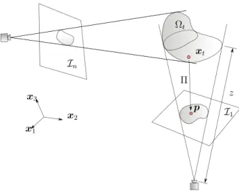
We assume that we are recording a scene with a standard, perspective projection video camera (RGBD cameras, for instance, are not considered in this work) [5]. This camera is producing, after calibration and lens distortion correction [29], as it moves, two-dimensional images of the three-dimensional environment. The passage from the three-dimensional world to the flat, two-dimensional images are actually a perspective projection, which we will denote by Π . The Structure from Motion, SfM, problem consists in determining the three-dimensional structure of a rigid scene from a sequence of images taken from different points of view, seeFig. 2.
The input image space is denoted by Ii ⊂ R2, with i = 1, . . . , nimages, the number of available images. This
number of images is in general growing continuously while we record with our camera, since a batch approach is in general not allowed in this work.
The a priori unknown camera operator is here denoted by Π :∂∗Ω
t →I. This camera projection can be expressed
as Π = K[R|t], where K corresponds to the camera intrinsic matrix and [R|t] represents the camera extrinsic matrix. By denoting xc t =(x, y, z) ⊤and p = ( p 1, p2)⊤we have, ⎡ ⎣ p1 p2 p3 ⎤ ⎦ =λ ⎡ ⎣ f/ dx 0 cx 0 f/dy cy 0 0 1 ⎤ ⎦ [R t 0 1 ] ⎡ ⎢ ⎢ ⎣ x y z 1 ⎤ ⎥ ⎥ ⎦ , where xc
t represents the coordinates of xt in the camera system (a moving frame of reference attached to the camera,
not to be confused with the world reference frame, depicted inFig. 2).∂∗Ω
t denotes the visible part of the boundary
of the object of interest, Ω , at time t . The camera extrinsic matrix transforms 3D scene points into 3D points in the camera reference. It establishes the rotation (R) and translation (t) between the corresponding points. The camera intrinsic matrix K contains information about the projection center (cx, cy), the pixel size (dx, dy) and the focal
distance ( f ), which is used to map 3D camera points into 2D pixel coordinates. The whole equation makes possible the transformation of real 3D points into image pixels. Finally,λ represents a scale factor.
Fig. 2. Sketch of the Structure from Motion problem.
Remark 1. Note that we have introduced two indexes, i and t, that may lead to confusion. i is purely discrete and refers to the frame number. On the contrary, t refers to time, and is therefore continuous. It will be subsequently discretized, of course, but even in this case, i and t need not to refer to the same quantity, nor the intervals ∆t and [i, i + 1] need to be of the same length. Once discretized, frame i captures time instant t, and sometimes we employ them indistinctly in an abuse of notation, but these indexes should not be confused.
Note that, with one single image, there is no way to determine if the image in the picture, p, has been produced by a big object located far away from the camera or a smaller one located close to it. To locate both the camera (its pose: position and orientation) and a rigid object we need more than one single image. One of the key ingredients of the SfM problem is the minimization of the reprojection error, i.e., the geometric error corresponding to the image distance between a projected point and a measured one [5]. As sketched inFig. 2, when a camera captures a picture of the environment, it is actually performing a projection of the 3d points in the form
p = Π (x),
with p ∈ R2and x ∈ R3(we omit for simplicity the superscript t ). However, in practice we do not know exactly the true value of x. It can be estimated by using well-known computer vision techniques, so as to give an estimate ˆx of the true 3d position of the point. The interested reader can consult [29] or [5], for instance. We therefore can think of a projection (re-projection, in fact) of this estimate, for each frame,
ˆ
p = Π (ˆx),
such that the reprojection error would be d(p, ˆp). In this work we are employing different techniques to determine the pose of the camera and to construct a map of the environment. This is indeed an intended choice, just to show that the proposed method works for any SfM problem. In the final example we show how the proposed method does not need any fiducial marker, as it employs the ORB-SLAM algorithm developed in [30].
When a deformable solid is located in the scene things become more intricate. A deforming solid is equivalent to having one single image pt per configuration xt = φ(X, t), and thus the problem becomes ill-posed. It is not
possible, in general, to determine the three-dimensional geometry of a solid with one single image. However, since we take pictures every 1/30 seconds, every configuration in the sequence of images, despite not being identical, is indeed very similar to the previous ones. An impressive effort of research has been devoted to solving the so-called Non-Rigid Structure from Motion (NRSfM) problem. A non-exhaustive list of techniques in this field could consider the Shape from Template (SfT) techniques [8,9], an Extended Kalman Filter approach employing linear elastic plate finite element to simulate the visible surface of the solid [6,31], or recent low-rank approaches to the that initialize the sequence with rigid motion only and sequentially improve the basis of the method [32], to name a few.
2.2. Assimilation of the data
Our approach to the problem will be that of deterministic data assimilation [24,33]. Even if it is possible to cast the problem in a Bayesian framework (see, for instance, some recent references that employ different types of Kalman filters in the context of reduced order modeling, [34–36]) we assume that observations coming from video streams are exact. Measurements coming from the NRSfM problem are indeed displacements of those points identified as belonging to deformable media. This constitutes a set of punctual displacements u∗.
Under this rationale, we consider the parametric dependence of the solution on a set of parametersµ ∈ D ⊂ Rnparam. These parameters will represent some hidden information to the user, such as the position of a load, for instance, that may be not visible in any of the frames. From the video stream, any of the aforementioned NRSfM techniques will provide a set of measurements –typically, displacements at some particular positions in the solid – by minimizing the reprojection error, for instance. These will be denoted as u∗(µ). The problem will be given by the following two discretized PDEs:
State equation: A(u, µ)u(x, µ) = f(µ),
Observation equation: u∗(µ) = C(µ)u(x, µ). (1)
We highlight here the fact that the stiffness matrix A(u, µ) could depend (possibly in a non-linear manner) both on the unknown field u (usually, the displacement field) and the parametersµ. u ∈ RnFOM represents the set of nodal (finite element full order model) degrees of freedom and u∗
∈ Rnobs represents the set of observations taken from the video stream. The observation matrix C is assumed to be linear and is usually simply Boolean andµ-independent.
The deterministic approach to this (inverse) problem could thus be cast in the following form: µ∗= argmin µ∈Rnparam 1 2∥u ∗− C(µ)u(x, µ)∥22, (2)
i.e., we seek to minimize the discrepancy between the observations u∗ and the model predictions u(µ) at particular locations given by matrix C. Frequently, this formulation is regularized by employing Tikhonov methods [14], but in this case we have not found it necessary.
The computational complexity of problem (2) prevents nowadays computers to obtain the desired feedback response at 30 Hz. This is so, at least, for state-of-the-art (possibly non-linear) models involving hundreds of thousands (if not millions) of degrees of freedom. This is at the origin of the need for some type of model order reduction. In this work, we have employed Proper Generalized Decompositions, whose basics are reviewed next. This will allow us to avoid the usage of high dimensional vectors u ∈ RnFOM, but to substitute them by surrogate reduced order approximations u ∈ RnROM, with nROM≪ nFOM.
3. A brief review of proper generalized decomposition
We will not go into every detail concerning Proper Generalized Decompositions, given the vast corps of literature available since the initial proposition of the method in [37] and its subsequent identification with the strategy also proposed by P. Ladeveze as an ingredient of his famous LaTIn method [16]. The interested reader can consult recent books on the methods such as [17,19,38] or review papers such as [20,39].
The essential ingredient in PGD methods is the assumption that the solution can be expressed as a finite sum of separate functions or, in other words, that the field u(x, µ) admits an affine parametric dependence, i.e.,
u(x, µ) ≈ nmodes ∑ i =1 Fi(x) ◦ G1i(µ1) ◦. . . ◦ G nparam i (µnparam), (3)
where the symbol “◦” represents the Hadamard or Schur component-wise product. Functions Fi, G j
i are also known as
“modes” to highlight their strong link to the modes employed in Proper Orthogonal Decomposition-based model order reduction methods. To determine their precise expression, Eq.(3)is substituted into the weak form of the problem at hand, from which Eq. ((1).a) emanates. Let us assume that the strong form of the problem is: find u(x, µ) in an appropriate functional space such that
equipped with suitable boundary conditions. Here, L represents the differential operator acting on the essential variable, u(x, µ). The precise form of this operator will be made clear for each of the examples in Section5. To obtain the weak form of the problem, we multiply both sides by a test function and integrate over the high-dimensional domain,
∫
Ωx×Ω1×···×Ωnparam
u∗(L(u) − f )dx dµ1· · ·dµnparam =0 ∀u
∗∈
H1
0(Ωx) × L2(µ). (4)
The separated form assumed for u, when substituted into Eq.(4), allows to perform integration in a separated manner. Of course, for this to be possible, the operator L must satisfy some separability assumptions as well. We refer the interested reader to [40] for a detailed analysis on the separability of differential operators, or to [41] in a hyperelastic context. We thus proceed by assuming that a rank-n approximation has just been constructed,
un(x, µ) = n ∑ i =1 Fi(x) ◦ G1i(µ1) ◦. . . ◦ G nparam i (µnparam), and look for a rank-1 improvement,
un+1(x, µ) = un(x, µ) + Fn+1(x) ◦ G1n+1(µ1) ◦. . . ◦ G nparam
n+1 (µnparam). In this same spirit, the test function will look
u∗(x, µ) = F∗n+1(x) ◦ G1n+1(µ1) ◦. . . ◦ G nparam n+1 (µnparam) +Fn+1(x) ◦ (G1n+1) ∗ (µ1) ◦. . . ◦ G nparam n+1 (µnparam) + · · · +Fn+1(x) ◦ G1n+1(µ1) ◦. . . ◦ (G nparam n+1 ) ∗(µ nparam).
Once substituted into Eq. (5.1), the assumed separated form of the unknown and the test function allow to perform the integration also in a separated way. The PGD algorithm is thus comprised by a greedy loop to determine the approximating sum plus a fixed-point, alternated directions scheme to find each of the modes. The interested reader could consult any of the mentioned references for further details and, in particular, [19] or [42] for detailed Matlab implementations.
In order to determine the number of modes in the approximation, n, a stopping criterion is mandatory. Error estimators have been proposed for PGD approximations that could be employed to this end [43–45].
4. PGD-based data assimilation
The procedure previously reviewed allows us to substitute u in Eq. (1.a) by its just computed rank-n approximation. Since this approximation is computed off-line and once for life, the savings in computational cost is usually of several orders of magnitude. Once a reduced-order approximation to u has been determined, the minimization in Eq.(2)is performed here by employing the well-known Levenberg–Marquardt method [25,27,46]. In this method, one has to determine the sensibilities of the solution with respect to the optimization parameters, i.e.,
∂u ∂µj (x, µ) ≈ n ∑ i =1 Fi(x) ◦ G1i(µ1) ◦. . . ◦ ∂Gj i(µj) ∂µj ◦. . . ◦ Gniparam(µnparam).
Thanks to the separated (affine) structure of the parametric dependence, sensibilities could also be computed off-line and stored in memory so as to be particularized during the runtime procedure. The reader can notice the extremely well suited structure of PGD approximations for such type of inverse problems.
In what follows we introduce three different examples in linear and non-linear elasticity that show the performance of the method and its suitability for augmented reality applications.
5. Examples
5.1. A linear elastic example employing fiducial markers
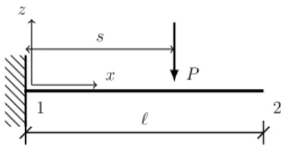
The first example is a linear elastic cantilever beam subjected to a punctual load applied at a variable position s, see the sketch inFig. 3.
Fig. 3. Cantilever beam problem. A moving load P is parameterized through its position coordinate s.
The beam is made of aluminum (Young’s modulus = 69 GPa, Poisson ratioν = 0.334) and the experiments were conducted in the linear elastic regime. The displacement field was assumed to have a form
u = u(x, s),
where x ∈ Ω represents the coordinates of the considered point and s the position of the applied load along the upper face of the beam, seeFig. 3. Following standard PGD postulates, an approximation of this parametric displacement field of the type
u(x, s) ≈
n
∑
i =1
Fi(x)Gi(s)
was computed. In this case the classical elasticity problem is assumed to govern the physics. Its weak form consists in finding the displacement u ∈ H1(Ω ) × L
2(Γt2) such that for all u∗∈H10×L2(Γt2):
∫ Γ ∫ Ω ∇su∗:σdΩdΓ = ∫ Γ ∫ Γt2 u∗·tdΓ dΓ
where Γ = Γu ∪Γt represents the boundary of the beam, divided into essential and natural regions, and where
Γt =Γt1∪Γt2, i.e., regions of homogeneous and non-homogeneous, respectively, natural boundary conditions. Here,
t = P ·δ(x − s)ek, whereδ represents the Dirac-delta function and ekthe unit vector along the z-coordinate axis (we
consider here, for the ease of exposition, a load P directed towards the negative z axis of reference).
Once regularized, the Dirac-delta term is approximated by a truncated series of separable functions in the spirit of the PGD method, i.e.,
tj ≈ m
∑
i =1
fji(x)gij(s)
where m represents the order of truncation and fi j, g
i
jrepresent the j th component of vectorial functions in space and
boundary position, respectively. For this particular example, only j = k (i.e., the third component of the vector) is assumed to exist.
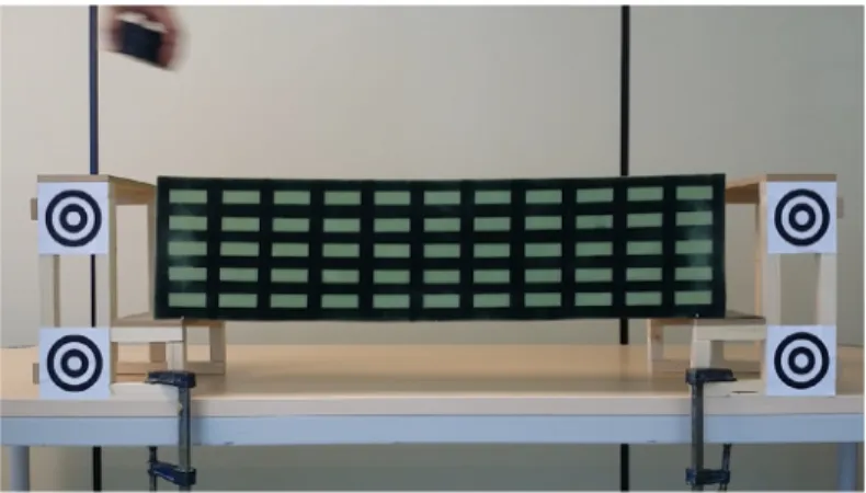
In this example, fiducial markers were employed to help locate the deformed configuration of the beam. SeeFig. 4
for a picture of the experimental device.
The use of fiducial markers is particularly advantageous for some industrial applications (structural health monitoring, for instance), for which there is no limitation to the presence of small adhered paper or plastic pieces, for instance. If this is not possible –for aesthetic reasons, for instance, or just because we have no a priori access to the studied solid – feature-based approaches must be preferred. These will be analyzed in Section5.3.
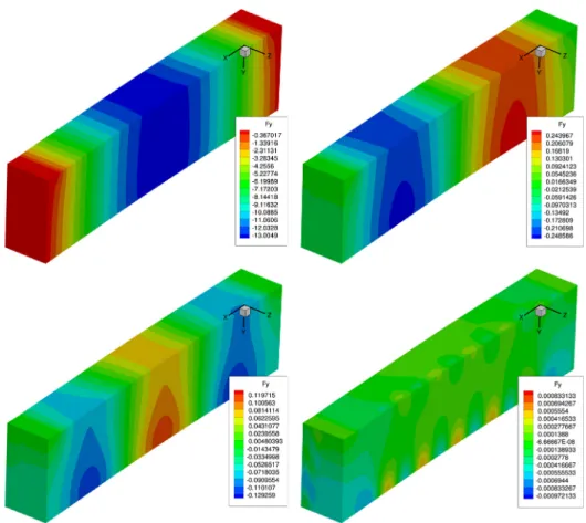
The number of modes n employed in this example was 19, even if for this problem much less are enough –see the big relative decay in modulus of the modes –. The first four spatial modes are represented inFig. 5, while modes on s are depicted inFig. 6.
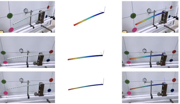
Results of the real-time assimilation procedure are reported inFig. 7, where different snapshots of the raw video, assimilated load position and augmented video are reported. Quantitative results are included inTable 1. Note that the reported errors are absolute and represent the difference between the assimilated load position and the actual one. Except for load positions very close to the clamped support, that produce almost no deflection in the beam, and therefore a large error in the assimilation procedure, errors are less than 1% for most positions (for instance, 0.3% error for the load at s = 460 mm, or 0.1% for s = 420 mm). These values can be improved by employing more PGD
Fig. 4. Experimental device for the aluminum beam example. Note the fiducial markers for the location of the beam and camera pose determination (big four circles) and the markers (small blue dots adhered to the beam) for the determination of the beam deflection.
Fig. 5. Modes Fi(x), i = 1, 2, 3, 4 for the aluminum beam example. These are vectorial modes. The color map corresponds to the vertical
displacement, the most relevant one.
Fig. 6. Modes Gi(s), i = 1, . . . , 5, for the aluminum beam problem.
modes, on one side, but are strongly limited by the camera’s resolution and the proximity of the beam to the objective. In other words, it is the portion of the solid covered by a single pixel that usually determines the level of precision.
The resulting video can be consulted at https://youtu.be/BK0sHfvjITo. In it, the robustness of the proposed technique to the partial occlusion of some of the fiducial markers or even a total occlusion of the camera are tested. The system resulted to be very robust and recovered immediately the load position without any problem.
5.2. A hyperelastic example without fiducials
A 797.5 × 200 × 105 mm3foam beam was considered in this example. The beam was meshed from a picture of a
Fig. 7. Three different snapshots of the raw video (left column), simulation (center) and augmented video (right). The color map corresponds to the modulus of the displacement field.
Table 1
Experimental results for the cantilever beam problem. Actual load position versus assimilated one. Errors are absolute.
Actual Mean Difference Actual Mean Difference Position Estimated abs. value Position Estimated abs. value s(mm) Pos. (mm) s(mm) (mm) Pos. (mm) (mm) 0 0.14 0.14 260 262.21 2.21 20 7.98 12.02 280 281.10 1.10 40 26.64 13.36 300 301.30 1.30 60 57.66 2.34 320 320.44 0.44 80 82.09 2.09 340 338.33 1.67 100 102.54 2.54 360 358.57 1.43 120 122.67 2.67 380 383.49 3.49 140 143.89 3.89 400 401.35 1.35 160 164.55 4.55 420 420.70 0.70 180 182.25 2.25 440 440.27 0.27 200 204.27 4.27 460 458.40 1.60 220 222.75 2.75 480 477.69 2.31 240 242.22 2.22
An experimental campaign was accomplished so as to determine that its (homogenized) constitutive law could be assimilated to a Kirchhoff–Saint Venant law with E = 0.11 N/mm2 and Poisson coefficient ν = 0.2. The
Kirchhoff–Saint Venant model is characterized by the energy density functional given by
Ψ =λ
2(tr(E))
2+µE : E,
whereλ and µ are Lame’s constants and E the Green–Lagrange strain tensor. In this case, the weak form of the problem, from which Eq. (1.a) emanates, takes the form
∫ Γ ∫ Ω (t) E∗:C : EdΩ dΓ = ∫ Γ ∫ Γt2 u∗·tdΓ dΓ,
Fig. 8. Geometry of the foam beam under self-weight load. This image was taken as the reference configuration of the beam. Fiducial markers were employed at this stage, that were later eliminated, to determine the pose of the camera and help to construct the reference configuration of the beam.
whereC represents the fourth-order constitutive tensor. Given the non-linear strain measure E, the resulting problem
is inherently non-linear.
Despite the well-known limitations of the Kirchoff–Saint Venant law under compressive stresses, this law showed to fit much better than usual hyperelastic laws (neo-Hookean, Mooney–Rivlin) to the experiments. In fact, some mild viscoelastic effects were observed, that are responsible of some oscillations in the results –see the accompanying video –, but these were nevertheless neglected. For short-term periods, results showed to be in good accordance to this law, as will be detailed hereafter.
A mesh of 18, 938 nodes and 98, 863 linear tetrahedral elements was created. Boundary conditions were assimilated to a pinned support (foam–wood contact surface showed to be nearly an adhesion) on the leftmost 40 mm. On the right, a sliding support was accomplished by means of plastic laminates. 15 N loads were applied by means of lead disks with 80 mm diameter, whose size was considered in detail in the simulation (due to the weak stiffness of the foam, punctual loads provoked very poor results by greatly deforming the upper surface of the foam).
The goal of this experiment was to develop augmented reality videos under real-time constraints (no batch processing was allowed) in which the position of the load was determined and the displacement field was plotted on top of the actual geometry of the beam, so as to indicate the user its true magnitude. Therefore, the displacement field was –as in Section5.1–assumed to have a parametric form
u = u(x, s),
where x ∈ Ω represents the coordinates of the considered point and s the position of the applied load along the upper face of the beam. A PGD approximation of this parametric displacement field of the type
u(x, s) ≈
n
∑
i =1
Fi(x)Gi(s)
was constructed off-line. n = 19 modes were considered in this approximation, although some experiments with only 11 modes provided results with very similar levels of accuracy. The load position coordinate, s was assumed to be one-dimensional, since the load was placed centered on the upper surface of the beam. The mesh along this dimension comprised 60 nodes in the central part of the beam (a portion of 100 mm of the beam at the right and left ends was not considered, since the displacements provoked by the load in these regions was not perceptible, due to the absence of bending). A detailed derivation of the necessary linearization of the Kirchhoff–Saint Venant law under the PGD framework was accomplished in [47]. The reader is referred to this reference or to [19] for a complete Matlab implementation.
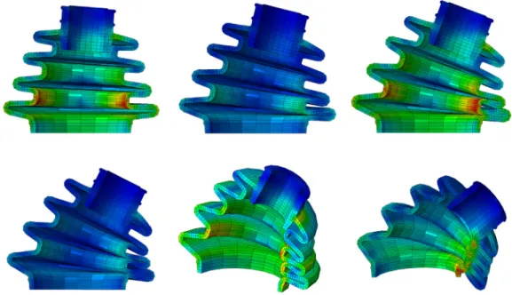
Fig. 9shows the first five Gi(s) modes of the model.Fig. 10shows modes Fi(x), i = 1, 2, 3 and 11.Fig. 11shows a
frame (second 55 of the video) in which we appreciate the accuracy of the assimilated displacement field and, notably, the location of the load position, marked with an arrow.
Fig. 9. Modes 1, 2, 3 and 11on s, the position of the load coordinate. Note that, as it is the case very often with PGD, the modes increase in frequency, the first one having the lowest frequency content.
Fig. 10. Modes Fi(x), i = 1, 2, 3 and 11 for the foam beam example. Again, modes increase in frequency as i increases. This a typical PGD result,
Fig. 11. Frame of the resulting video (second 55) in which we appreciate the assimilated position of the load (see the arrow). Superimposed, the displacement field of the beam. Note that no fiducial marker is employed at this stage.
The video was recorded at a resolution of 1280 × 720 p. (which is the resolution of an iPhone 6). Under these circumstances, the proposed method is able to provide a response at 60 Hz. The mean error is on the order of 1.5 mm. This value is also dependent on the relative proximity of the deformable object (the foam beam) to the camera, of course. In other words, to the actual, physical, displacement registered by each pixel in the image. This error could therefore be improved by augmenting the resolution of the camera, by taking a closer view or, once we have tried any of the previous possibilities, by increasing the number of modes in the approximation of the displacement field.
The resulting video has been made public athttps://www.youtube.com/watch?v=byhXy8aJ1J8. 5.3. Neo-Hookean hyperelasticity
We consider in this example the process of design and analysis of an automotive boot sealing made of a neo-Hookean rubber. The geometry of the seal is shown inFig. 12. The model is composed by a mesh of 8640 nodes and 5940 linear hexahedral elements. The rubber is assumed to follow an incompressible law
W = C1(I1−3),
where W represents the strain energy density function, C1=1166 MPa for this particular example, and I1represents
the first invariant of the right Cauchy–Green strain tensor. The material is thus considered incompressible. The lever is assumed to be rigid, and rotates around a pinned support in the plane where the boot seal lies.
In this particular example the boot seal does not exist physically in the video. Instead, this example opens the possibility of employing augmented reality for engineering design purposes, by showing the performance and appearance that the virtual object could have in the physical world.
In this particular example, the displacement field of the boot seal is parameterized by the angle of rotation of the lever,θ. As in the previous examples, we hypothesize that this dependence can be affinely approximated as
u(x, θ) ≈
n
∑
i =1
Fi(x)Gi(θ). (5)
5.3.1. Construction of the reduced order model
For this particular example, the so-called non-intrusive PGD method has been employed [49,50]. In particular, we have employed the formulation introduced in [50], that employs adaptive samplings of the parametric domain and collocation approaches. We thus avoid complex linearization procedures while employing off-the-shelf commercial softwares to construct the sought PGD approximation, Eq.(5). Some of the spatial modes Fi(x) are shown inFig. 13.
The parametric spaceθ ∈ [0◦, 52◦] –here, symmetry has been employed – has been discretized into 193 finite
elements. Probably much less degrees of freedom could be necessary but, given the inherent non-linearity of the problem due to the presence of contact phenomena, a very fine discretization was employed that nevertheless did not prevent the method to reach the real-time constraints.
Fig. 12. Geometry of the rubbery boot seal (left) and a snapshot during the process (right). The angleθ is the fundamental magnitude to be determined by the computer vision system, since the boot seal is entirely virtual. It does not exist in the physical reality.
Fig. 13. Different modes Fi(x), for the boot seal non intrusive approximation.
5.3.2. Segmentation and registration
In this example, as already mentioned repeatedly, there is no physical boot seal. Therefore, the objective of the computer vision implementation is to determine the degree of rotationθ of the lever. To that end, no fiducial markers have been employed. In the absence of that markers, computer vision systems employ feature matching algorithms, capable of detecting and tracking local frame features. In this work we employ ORB feature detectors [51]. These are the green markers inFig. 14. Within SLAM algorithms, ORB detectors provide with a very efficient means of unveiling the environment in which we move [30].
SLAM methods were primarily designed for robot navigation in rigid environments. But in this particular example the objective is to detect the lever tilt angleθ. In other words: there is some part of the scene that is not rigid. To detect θ an algorithm is proposed in which we proceed by parts. First of all, it is necessary to detect the plate in which the lever is mounted. To that end, we employ Random Sample Consensus (RANSAC) methods [52]. RANSAC methods allow to fit a model from experimental data in the presence of a big number of outliers. This is precisely our case: a significant portion of the ORB features lie on a plane (precisely the plate in which the lever is mounted), while the
Fig. 14. Raw video with the detected features in green. Note that there is no boot seal in the physical reality. (For interpretation of the references to color in this figure legend, the reader is referred to the web version of this article.)
Fig. 15. Detection by RANSAC methods of the plate where the lever is located (in red) and reconstruction of the rigid environment (in blue). (For interpretation of the references to color in this figure legend, the reader is referred to the web version of this article.)
rest of the detected features in the environment are considered outliers. The resulting detection is shown inFig. 15, where the detected plate is depicted by means of red features, while the environment is depicted in blue. InFig. 16the results of the ORB-SLAM [30] reconstruction of the environment, together with the found pose of the camera (blue squares) are shown. This method allows to track the movement of the camera in a very accurate manner.
Once the plate has been detected, the tilting angle of the lever is found by filtering the white color of the lever from the images. This allows for a very precise determination of the angleθ, seeFig. 17.
5.3.3. Performance
The resulting video from which frames in Fig. 17 have been extracted can be seen at https://youtu.be/0whA 92vFk1g. In it, a robustness test is made for the proposed method in which the camera is moved away of the
Fig. 16. Results of the ORB-SLAM tracking of the camera pose and reconstruction of the environment [30]. Red points represent the detected features, blue squares represent the camera pose at different time instants and the green lines indicate common found structures between frames. (For interpretation of the references to color in this figure legend, the reader is referred to the web version of this article.)
Fig. 17. Two different augmented frames of the video. Color map corresponds to the modulus of the displacement field at the plane of symmetry (right) and von Mises stresses (left).
lever position, so that it disappears from the image. The localization capabilities of ORB-SLAM methods are able, nevertheless, to find the lever back with great precision, thus closing the loop and restarting the augmentation with no problems.
6. Discussion
In this paper a new method for the physically realistic augmentation of video streams through numerical simulation is proposed. The method, given the stringent constraints imposed by modern video frame rates (30 or 60 frames per second in an iPhone, for instance) is based on the employ of reduced order modeling and simulation. In particular, the affine (separate) parametric approximation of most reduced order techniques is exploited for a very efficient data assimilation procedure that enables us to obtain a very accurate registration between reality and our model.
The proposed method is valid for any augmented reality application in which we are interested about hidden information in the video governed by a PDE (such as stress, for instance), but also to create and augment with objects not present in the physical reality. In any case, state-of-the-art computer vision techniques have been employed so as to detect the camera pose and to map the environment. Three different examples have been analyzed in which we employ different approaches to the problem of simultaneous localization and mapping of the environment. In the first of them we employed fiducial markers, a very versatile possibility in industrial settings, where we can mark the object of interest with such badges. In the second one we employed some existing pattern in the solid so as to track deformations in it, while in the third example we employed feature-based approaches (in particular, ORB-SLAM) to locate the solid, track its deformation and the camera pose.
In any of the three different examples, the usage of reduced order methods (here, Proper Generalized Decomposi-tions) allowed for a very efficient and accurate determination of the variables of interest at usual video frame rates. A standard iPhone 6 camera was employed for every example.
The presented method opens the door for more complex augmented reality applications that truly enable a linkage of simulation techniques with video formats, thus widening the possibilities of modern CAE techniques.
Acknowledgments
We are grateful to our colleague at the Aragon Institute of Engineering Research, prof. J. M. M. Montiel, whose guidance through the world of computer vision has been crucial to us. We are also grateful to Miguel ´Angel Varona and Eduardo Estopi˜n´an, whose help with the foam example is greatly appreciated.
References
[1] N. Haouchine, J. Dequidt, M.O. Berger, S. Cotin, Monocular 3D reconstruction and augmentation of elastic surfaces with self-occlusion handling, IEEE Trans. Vis. Comput. Graphics 21 (12) (2015) 1363–1376.
[2] N. Haouchine, S. Cotin, I. Peterlik, J. Dequidt, M.S. Lopez, E. Kerrien, M.O. Berger, Impact of soft tissue heterogeneity on augmented reality for liver surgery, IEEE Trans. Vis. Comput. Graphics 21 (5) (2015) 584–597.
[3] Abe Davis, Justin G. Chen, Frédo Durand, Image-space modal bases for plausible manipulation of objects in video, ACM Trans. Graph. 34 (6) (2015) 239:1–239:7.
[4] J. Civera, D.R. Bueno, A.J. Davison, J.M.M. Montiel, Camera self-calibration for sequential bayesian structure from motion, in: 2009 IEEE International Conference on Robotics and Automation, 2009.
[5] Richard Hartley, Andrew Zisserman, Multiple View Geometry in Computer Vision, Cambridge University Press, 2003.
[6] A. Agudo, F. Moreno-Noguer, B. Calvo, J.M.M. Montiel, Sequential non-rigid structure from motion using physical priors, IEEE Trans. Pattern Anal. Mach. Intell. 38 (5) (2016) 979–994.
[7] Antonio Agudo, Francesc Moreno-Noguer, Begoña Calvo, J.M.M. Montiel, Real-time 3d reconstruction of non-rigid shapes with a single moving camera, Comput. Vis. Image Underst. 153 (2016) 37–54. Special issue on Visual Tracking.
[8] A. Bartoli, Y. Gérard, F. Chadebecq, T. Collins, D. Pizarro, Shape-from-template, IEEE Trans. Pattern Anal. Mach. Intell. 37 (10) (2015) 2099–2118.
[9] A. Malti, A. Bartoli, R. Hartley, A linear least-squares solution to elastic shape-from-template, in: 2015 IEEE Conference on Computer Vision and Pattern Recognition (CVPR), 2015.
[10] A. Quarteroni, G. Rozza, A. Manzoni, Certified reduced basis approximation for parametrized pde and applications, J. Math. Ind. 3 (2011).
[11] Y. Maday, E.M. Ronquist, The reduced basis element method: application to a thermal fin problem, SIAM J. Sci. Comput. 26/1 (2004) 240–258.
[12] Y. Maday, A.T. Patera, G. Turinici, A priori convergence theory for reduced-basis approximations of single-parametric elliptic partial differential equations, J. Sci. Comput. 17/1-4 (2002) 437–446.
[13] A. Manzoni, S. Pagani, T. Lassila, Accurate solution of bayesian inverse uncertainty quantification problems combining reduced basis methods and reduction error models, SIAM/ASA J. Uncertain. Quantif. 4 (1) (2016) 380–412.
[14] Andrea Manzoni, Toni Lassila, Alfio Quarteroni, Gianluigi Rozza, A reduced-order strategy for solving inverse bayesian shape identification problems in physiological flows, in: Hans Georg Bock, Xuan Phu Hoang, Rolf Rannacher, Johannes P. Schl¨oder (Eds.), Modeling, Simulation and Optimization of Complex Processes - HPSC 2012: Proceedings of the Fifth International Conference on High Performance Scientific Computing, March 5-9, 2012, Hanoi, Vietnam, Springer International Publishing, Cham, 2014, pp. 145–155.
[15] A. Manzoni, A. Quarteroni, G. Rozza, Computational reduction for parametrized PDEs: Strategies and applications, Milan J. Math. 80 (2012) 283–309.
[16] P. Ladeveze, Nonlinear Computational Structural Mechanics, Springer, N.Y., 1999.
[17] Francisco Chinesta, Elias Cueto, PGD-Based Modeling of Materials, Structures and Processes, Springer International Publishing Switzerland, 2014.
[18] P. Ladeveze, J.-C. Passieux, D. Neron, The LATIN multiscale computational method and the Proper Generalized Decomposition, Comput. Methods Appl. Mech. Engrg. 199 (21–22) (2010) 1287–1296.
[19] E. Cueto, D. Gonz´alez, I. Alfaro, Proper generalized decompositions: an introduction to computer implementation with matlab, in: SpringerBriefs in Applied Sciences and Technology, Springer International Publishing, 2016.
[20] F. Chinesta, A. Ammar, E. Cueto, Recent advances in the use of the Proper Generalized Decomposition for solving multidimensional models, Arch. Comput. Methods Eng. 17 (4) (2010) 327–350.
[21] Pierre Ladeveze, Ludovic Chamoin, On the verification of model reduction methods based on the proper generalized decomposition, Comput. Methods Appl. Mech. Engrg. 200 (23-24) (2011) 2032–2047.
[22] Thomas L.D. Croft, Timothy N. Phillips, Least-squares proper generalized decompositions for weakly coercive elliptic problems, SIAM J. Sci. Comput. 39 (4) (2017) A1366–A1388.
[23] Alberto Bad´ıas, David Gonz´alez, Iciar Alfaro, Francisco Chinesta, Elias Cueto, Local proper generalized decomposition, Internat. J. Numer. Methods Engrg. 112 (12) (2017) 1715–1732.
[24] D. Gonzalez, F. Masson, F. Poulhaon, E. Cueto, F. Chinesta, Proper generalized decomposition based dynamic data driven inverse identification, Math. Comput. Simulation 82 (2012) 1677–1695.
[25] Amine Ammar, Antonio Huerta, Francisco Chinesta, El´ıas Cueto, Adrien Leygue, Parametric solutions involving geometry: A step towards efficient shape optimization, Comput. Methods Appl. Mech. Engrg. 268 (2014) 178–193.
[26] J.V. Aguado, A. Huerta, F. Chinesta, E. Cueto, Real-time monitoring of thermal processes by reduced order modelling, Internat. J. Numer. Methods Engrg. 102 (5) (2015) 991–1017.
[27] Ch. Ghnatios, F. Masson, A. Huerta, A. Leygue, E. Cueto, F. Chinesta, Proper generalized decomposition based dynamic data-driven control of thermal processes, Comput. Methods Appl. Mech. Engrg. 213–216 (2012) 29–41.
[28] Richard Szeliski, Computer Vision: Algorithms and Applications, Springer International Publishing, 2010.
[29] Gary Bradski, Adrian Kaehler, Learning OpenCV: Computer vision with the OpenCV library, O’Reilly Media, Inc., 2008.
[30] R. Mur-Artal, J.M.M. Montiel, J.D. Tard´os, ORB-SLAM: A versatile and accurate monocular SLAM system, IEEE Trans. Robot. 31 (5) (2015) 1552–3098.
[31] Antonio Agudo, Francesc Moreno-Noguer, Bego˜na Calvo, J.M.M. Montiel, Real-time 3D reconstruction of non-rigid shapes with a single moving camera, Comput. Vis. Image Underst. 153 (Supplement C) (2016) 37–54. Special issue on Visual Tracking.
[32] Marco Paladini, Adrien Bartoli, Lourdes Agapito, Sequential non-rigid structure-from-motion with the 3D-implicit low-rank shape model, in: Kostas Daniilidis, Petros Maragos, Nikos Paragios (Eds.), Computer Vision –ECCV 2010: 11th European Conference on Computer Vision, Heraklion, Crete, Greece, September 5-11, 2010, Proceedings, Part II, Springer, Berlin, Heidelberg, 2010, pp. 15–28.
[33] E. Nadal, F. Chinesta, P. D´ıez, F.J. Fuenmayor, F.D. Denia, Real time parameter identification and solution reconstruction from experimental data using the proper generalized decomposition, Comput. Methods Appl. Mech. Engrg. 296 (2015) 113–128.
[34] Basile Marchand, Ludovic Chamoin, Christian Rey, Real-time updating of structural mechanics models using kalman filtering, modified constitutive relation error, and proper generalized decomposition, Internat. J. Numer. Methods Engrg. 107 (9) (2016) 786–810.
[35] Philippe Moireau, Dominique Chapelle, Reduced-order Unscented Kalman Filtering with application to parameter identification in large-dimensional systems, ESAIM Control Optim. Calc. Var. 17 (2) (2011) 380–405. See also erratum DOI:http://dx.doi.org/10.1051/cocv/2011 001.
[36] David Gonz´alez, Alberto Bad´ıas, Ic´ıar Alfaro, Francisco Chinesta, El´ıas Cueto, Model order reduction for real-time data assimilation through Extended Kalman Filters, Comput. Methods Appl. Mech. Engrg. 326 (Supplement C) (2017) 679–693.
[37] A. Ammar, B. Mokdad, F. Chinesta, R. Keunings, A new family of solvers for some classes of multidimensional partial differential equations encountered in kinetic theory modeling of complex fluids, J. Non-Newtonian Fluid Mech. 139 (2006) 153–176.
[38] F. Chinesta, P. Ladeveze (Eds.), Separated Representations and PGD-Based Model Reduction, Springer International Publishing, 2014.
[39] Francisco Chinesta, Pierre Ladeveze, Elias Cueto, A short review on model order reduction based on proper generalized decomposition, Arch. Comput. Methods Eng. 18 (2011) 395–404.
[40] David Modesto, Sergio Zlotnik, Antonio Huerta, Proper generalized decomposition for parameterized helmholtz problems in heterogeneous and unbounded domains: application to harbor agitation, Comput. Methods Appl. Mech. Engrg. 295 (2015) 127–149.
[41] S. Niroomandi, D. Gonzalez, I. Alfaro, E. Cueto, F. Chinesta, Model order reduction in hyperelasticity: a proper generalized decomposition approach, Internat. J. Numer. Methods Engrg. 96 (3) (2013) 129–149.
[42] Francisco Chinesta, Roland Keunings, Adrien Leygue, The proper generalized decomposition for advanced numerical simulations, Springer International Publishing Switzerland, 2014.
[43] A. Ammar, F. Chinesta, P. Diez, A. Huerta, An error estimator for separated representations of highly multidimensional models, Comput. Methods Appl. Mech. Engrg. 199 (25–28) (2010) 1872–1880.
[44] Iciar Alfaro, David Gonzalez, Sergio Zlotnik, Pedro Diez, Elias Cueto, Francisco Chinesta, An error estimator for real-time simulators based on model order reduction, Adv. Model. Simul. Eng. Sci. 2 (1) (2015) 30.
[45] J.P. Moitinho de Almeida, A basis for bounding the errors of proper generalised decomposition solutions in solid mechanics, Internat. J. Numer. Methods Engrg. 94 (10) (2013) 961–984.
[46] F. Chinesta, A. Leygue, F. Bordeu, J.V. Aguado, E. Cueto, D. Gonzalez, I. Alfaro, A. Ammar, A. Huerta, PGD-based computational vademecum for efficient design, optimization and control, Arch. Comput. Methods Eng. 20 (1) (2013) 31–59.
[47] S. Niroomandi, D. Gonz´alez, I. Alfaro, F. Bordeu, A. Leygue, E. Cueto, F. Chinesta, Real-time simulation of biological soft tissues: a PGD approach, Int. J. Numer. Methods Biomed. Eng. 29 (5) (2013) 586–600.
[48] Siamak Niroomandi, Iciar Alfaro, Elias Cueto, Francisco Chinesta, Model order reduction for hyperelastic materials, Internat. J. Numer. Methods Engrg. 81 (9) (2010) 1180–1206.
[49] X. Zou, M. Conti, P. D´ıez, F. Auricchio, A nonintrusive proper generalized decomposition scheme with application in biomechanics, Internat. J. Numer. Methods Engrg. 113 (2) (2018) 230–251.
[50] Domenico Borzacchiello, Jos´e V. Aguado, Francisco Chinesta, Non-intrusive sparse subspace learning for parametrized problems, Arch. Comput. Methods Eng. (2017).
[51] E. Rublee, V. Rabaud, K. Konolige, G. Bradski, ORB: An efficient alternative to SIFT or SURF, in: 2011 International Conference on Computer Vision, 2011, pp. 2564–2571.
[52] Martin A. Fischler, Robert C. Bolles, Random sample consensus: a paradigm for model fitting with applications to image analysis and automated cartography, Commun. ACM 24 (6) (1981) 381–395.