HAL Id: tel-03178308
https://tel.archives-ouvertes.fr/tel-03178308
Submitted on 23 Mar 2021HAL is a multi-disciplinary open access archive for the deposit and dissemination of sci-entific research documents, whether they are pub-lished or not. The documents may come from teaching and research institutions in France or
L’archive ouverte pluridisciplinaire HAL, est destinée au dépôt et à la diffusion de documents scientifiques de niveau recherche, publiés ou non, émanant des établissements d’enseignement et de recherche français ou étrangers, des laboratoires
Qiuyue Luo
To cite this version:
Qiuyue Luo. Self-stabilization of 3D Walking of a Biped Robot. Robotics [cs.RO]. École centrale de Nantes, 2020. English. �NNT : 2020ECDN0010�. �tel-03178308�
T
HÈSE DE DOCTORAT DE
L’ÉCOLE CENTRALE DE NANTES
ÉCOLE DOCTORALE N° 601
Mathématiques et Sciences et Technologies de l’Information et de la Communication
Spécialité : Automatique Productique et Robotique Par
« Qiuyue LUO »
« Marche Bipède 3D Auto-Stabilisante »
« Self-stabilization of 3D walking of a biped robot »
Thèse présentée et soutenue à « L’École Centrale de Nantes», le « 18/06/2020 »
Unité de recherche : UMR 6004, Laboratoire des Sciences du Numérique de Nantes (LS2N)
Rapporteurs avant soutenance :
Olivier Stasse, Directeur de recherche, LAAS, Toulouse
Andrea Cherubini, Maître de conférences HDR, Université de Montpellier Composition du Jury :
Président : Claude Moog Directeur de recherche, CNRS, École Centrale de Nantes
Examinateurs : Olivier Stasse Directeur de recherche, LAAS, Toulouse
Andrea Cherubini Maître de conférences HDR, Université de Montpellier Jean Paul Laumond Directeur de recherche, INRIA, Paris
Yannick Aoustin Professeur des Universités, Université de Nantes
CONTEXTE ET ORGANISATION DE
LA THÈSE
Motivation
Les robots humanoïdes, bien adaptés pour évoluer dans les milieux humains, peuvent avec leurs bras et mains effectuer des tâches complexes. Ils peuvent être considérés comme l’un des robots ultimes. Ils suscitent un grand engouement dans la société humaine car ils peuvent devenir des partenaires très utiles dans le quotidien et en milieux industriels. Cependant, la marche bipède reste un phénomène complexe qui n’a pas été entièrement compris. Les robots humanoïdes étant des systèmes très complexes avec des degrés de liberté (ddl) élevés, de nombreux modèles simplifiés ont été étudiés. L’un des modèles les plus simples et les plus populaires est le modèle pendule inversé linéaire (LIP) [1]. Avec le modèle LIP, le robot est supposé être une masse concentrée avec une accélération verticale nulle du centre de masse (CdM), des pieds pointus et des jambes sans masse. Une approche de commande classique est le modèle de commande prédictif (MCP) [2], qui a été utilisé pour de nombreux robots humanoïdes avec des pieds. Il peut être adapté dans de nombreux environnements complexes. Une autre méthode populaire est fondée sur les approches qui utilisent le point de capture (CP) [3] qui fonctionnent bien pour rejeter une perturbation comme une poussée extérieure appliquée au robot humanoïde. Ces approches, y compris certaines méthodes de commande basées sur l’optimisation [4], sont appelées commande de haut niveau, qui se réfère à des approches basées sur la prédiction des états futurs du CdM et des emplacements des pieds.
On sait que la marche des humains sur un sol relativement plat ne nécessite pas d’attention [5] et il existe une phase de déséquilibre pendant la marche. La stabilité de marche des êtres humains est obtenue en changeant alternativement la jambe de position. Un problème canonique est de savoir comment concevoir un correcteur basé sur la phase de déséquilibre. L’approche de commande basée sur les contraintes virtuelles [6] est un bon outil pour étudier ce problème. Les contraintes virtuelles sont les relations fonctionnelles entre les états du système, c’est-à-dire que les variables commandées sont définies comme
du temps. Cela signifie que lorsqu’une démarche est perturbée, le système n’a pas à se resynchroniser avec le temps après la perturbation. Avec un bon choix de contraintes virtuelles, une auto-synchronisation et une auto-stabilisation peuvent être obtenues. Les notions d’auto-synchronisation et d’auto-stabilisation se réfèrent à la synchronisation et à la stabilité obtenues sans commande de haut niveau mentionné précédemment. La notion d’auto-synchronisation qui a été proposée par Razavi et al. [7], se réfère aux périodes des mouvements pendulaires dans les plans sagittal et frontal tendant à une période commune. En 2000, un groupe de laboratoires français comprenant Irccyn (l’ancien nom de LS2N) avec Université du Michigan (UM) construit Rabbit [8], qui est un robot planaire avec 5 corps et 4 actionneurs. Il y a donc 1 degré de sous-actionnement lors d’un simple appui du robot bipède sur le sol. Notez que comme il n’y a pas d’actionnement aux extrémités des jambes, ce qui fait avancer le robot est la gravité. Pour Rabbit, les quatre articulations actionnées sont choisies comme variables commandées. Un autre choix peut être la position du pied pivotant dans l’espace Cartésien ou l’orientation du torse. La variable de phasage doit être monotone. Ainsi, l’angle entre l’axe vertical et la ligne reliant le pied d’appui et la position CdM de la hanche ou sagittale peut être choisi comme variable de mise en phase. Lorsque les variables commandées suivent parfaitement l’évolution souhaitée, un système d’ordre réduit peut être obtenu, appelé dynamique zéro hybride (HZD) [9]. Dans les travaux de Chevallereau et Aoustin [10], il a été prouvé que dans l’espace 2D, la stabilité est obtenue si la vitesse du CdM est dirigée vers le bas à la fin d’une étape.
L’objectif général de la thèse est d’essayer de comprendre les conditions physiques que les allures doivent satisfaire dans l’espace 3D pour maintenir la stabilité dans la marche périodique, et de produire une stratégie de commande avec laquelle l’auto-synchronisation et l’auto-stabilisation peuvent être obtenues.
Organisation de la thèse
— Dans la première partie (Chapitre 2), le LIP modèle est utilisé pour étudier les stratégies de commande. L’influence du placement du pied libre sur le sol et les conditions de changement de jambe d’appui, en fonction du temps ou de l’état in-terne du robot sont étudiées. Il est montré que ni synchronisation ni l’auto-stabilisation ne sont observées lorsque la commutation de jambe d’appui est fondée sur le temps ou lorsque la longueur et la largeur de pas sont fixes. D’autre part,
l’auto-synchronisation peut être obtenue lorsque la condition de transfert de la jambe d’appui est fondée sur une combinaison linéaire des positions du CdM le long des axes sagittal et frontal. De plus, l’auto-stabilisation peut être obtenue lorsque la vitesse du CdM dans le plan sagittal est prise en compte. Lorsque l’auto-stabilisation est obtenue, aucune méthode de commande du haut niveau n’est requise.
— Dans la deuxième partie (Chapitre 3), afin d’analyser l’influence de l’oscillation verticale du CdM du robot sur la stabilité de marche, le modèle de pendule inversé de longueur variable (VLIP) est utilisé. Il est démontré que l’oscillation verticale du CdM, le placement du pied libre et le choix de la condition de transfert jouent un rôle crucial dans la stabilité. De plus, un correcteur proportionnel intégral (PI) en fonction de la vitesse du CdM le long de l’axe sagittal est également proposé de telle sorte que la vitesse de marche du robot puisse converger vers un mouvement périodique choisi avec une vitesse de marche donnée.
— Dans la dernière partie (Chapitres 4-5) un nouveau modèle de marche, nommé le modèle essentiel est proposé. Il a la même dimension que le modèle 3D LIP mais il prend en compte la dynamique complète de l’humanoïde. Le modèle es-sentiel définit la dynamique de la position horizontale du CdM en fonction d’une trajectoire souhaitée du zéro moment point (ZMP). Les trajectoires de référence des variables commandées sont définies en fonction des états internes du robot et/ou d’informations externes, générant ainsi des modèles à des fins différentes. La stratégie de commande proposée pour les modèles LIP et VLIP est étendue à travers le modèle essentiel pour commander un modèle humanoïde complet. L’introduction du modèle complet modifie légèrement la gamme des paramètres qui conduisent à des allures auto-stables. L’algorithme de marche proposé ci-dessus est appliqué sur les robots humanoïdes Roméo et TALOS.
Certains des résultats de la thèse ont été publiés ou acceptés dans des conférences ou des revues.
Revues internationales
— Q. Luo, V. De-León-Gómez, A. Kalouguine, C. Chevallereau and Y. Aoustin,
Self-Synchronization and Self-Stabilization of Walking Gaits Modeled by the Three-Dimensional LIP Model[J], dans IEEE Robotics and Automation Letters, 2018,
verted Pendulum Controlled with Virtual Constraints[J], dans International Journal
of Humanoid Robotics, Vol. 16, No. 06, 1950040 (2019)
— V. De-León-Gómez, Q. Luo, A. Kalouguine, J.A. Pámanes, Y. Aoustin, and C. Chevallereau, An essential model for generating walking motions for humanoid
robots[J], dans Robotics and Autonomous Systems, 2019, 112: 229-243.
Conférences internationales
— Q. Luo, V. De-León-Gómez, A. Kalouguine, C. Chevallereau, and Y. Aoustin,
Self-Synchronization and Self-Stabilization of Walking Gaits Modeled by the Three-Dimensional LIP Model, communiqué dans 2018 IEEE/RSJ International
A
CKNOWLEDGEMENT
My deepest gratitude goes first to my supervisor Prof. Christine Chevallereau and Prof. Yannick Aoustin who have put their valuable experience and wisdom at my disposal. They provided critical advices in my researches and suggested many important additions and improvements. It has been a greatly enriching experience to me to work under their authoritative guidance. I also thank Dr. Víctor De-León-Gómez and Dr. Anne Kalouguine for their suggestions and comments of my research work. I have spent a great time working with them.
I would also like to express my gratitude to the China Scholarship Council (CSC) for providing me the financial support during the three years.
I want to thank Dr. Abhilash Nayak, Mario Ciranni, Yang Deng, Vamsi Krishna GUDA, Yankai Xing for sharing their knowledge with me and helping sloving my con-fusions when I met a problem in my work. In Nantes, I am lucky to have many friends from China who are studying in different research areas so that we can share different stories and life experiences together. Thank you all for caring about me and the sincere encouragement.
Last but not least, I want to express my gratitude to my parents, who encourage me to pursuing the PhD for the subject I am passionate about, with their endless love and selfless support.
A
BSTRACT
Humanoid robot, which can walk by two legs and perform skillful tasks using both arms with hands, could be considered as one of the ultimate robots. They are especially desirable in human society as they can work well in the environments that have been de-signed for humans, and become our partners. However, bipedal walking remains a complex phenomenon that has not been fully understood.
The thesis is dedicated to find some physical insights that can explain the stability of periodic walking on horizontal floor. In human walking, the gait is usually expressed as a function of a phasing variable based on the internal state instead of time. The controlled variables (swing foot trajectories, vertical oscillation of center of mass, upper body motion, etc.) of the robots are based on a phasing variable via the use of virtual constraints and the step timing is not explicitly imposed but implicitly adapted under disturbances.
In the first part, a simplified model of the robot: the linear inverted pendulum (LIP) model is used to study control strategies. Landing positions of the swing foot, and con-ditions to switch the stance leg, based on time or on the internal state of the robot are studied. It is shown that neither self-synchronization nor self-stabilization is observed when the stance leg switching is based on time or when both the step length and width are fixed. On the other hand, self-synchronization can be obtained when the switching condition of the stance leg is based on a linear combination of the positions of the center of mass (CoM) along the sagittal and frontal axes. Moreover, self-stabilization can be obtained when the velocity of the CoM in the sagittal plane is taken into account. When self-stabilization is obtained, no high-level control methods are required (such as model predictive control, capture point-based control, optimization-based control etc.).
In order to analyze the influence of the vertical oscillation of the robot CoM on walking stability, the variable length inverted pendulum (VLIP) model is used. It is shown that the vertical CoM oscillation, positions of the swing foot and the choice of the switching condition play a crucial role in stability. Moreover, a PI controller of the CoM velocity along the sagittal axis is also proposed such that the walking speed of the robot can converge to a chosen periodic motion with a given walking speed.
humanoid. It can be written based on the internal states of the robot and possible external information, thereby generating models for different purposes. The essential model defines the dynamics of the horizontal position of the CoM as a function of a desired trajectory of the ZMP, assuming a perfect tracking of the reference trajectories. The proposed control strategy for the LIP and VLIP models is extended through the essential model to control a complete humanoid model. Introducing the complete model modifies slightly the range of parameters leading to self-stable gaits. The walking algorithm proposed above is applied on the humanoid robots Romeo and TALOS.
Key words: Humanoid and bipedal locomotion, passive walking, dynamic stability, hybrid systems, modeling
T
ABLE OF
C
ONTENTS
1 Introduction 15
1.1 Background . . . 15
1.2 The development of humanoid robots . . . 16
1.3 Gait patern generation . . . 19
1.3.1 Control with Simplified model . . . 19
1.3.2 Passive based control . . . 20
1.3.3 Virtual constraints and hybrid zero dynamics (HZD) . . . 21
1.4 Overview and outlines of the dissertation . . . 22
1.5 Contributions of the dissertation . . . 23
2 Self-synchronization and self-stability of LIP model 25 2.1 Introduction . . . 25
2.2 Modeling of the walking gait via LIP model . . . 26
2.2.1 General description. . . 26
2.2.2 Model in SS phase. . . 26
2.2.3 Transition between steps. . . 30
2.2.4 Hybrid model. . . 30
2.2.5 Periodic motion. . . 31
2.3 The swing foot motion . . . 32
2.3.1 The vertical swing foot motion. . . 33
2.3.2 The horizontal swing foot motion. . . 33
2.4 The Poincaré return map . . . 36
2.5 Transition based on time . . . 38
2.5.1 Stability study. . . 38
2.5.2 Simulation . . . 38
2.6 Transition based on the horizontal CoM position . . . 42
2.6.1 The virtual constraints . . . 42
2.6.2 The phasing variable . . . 43
2.6.4 Choice of C. . . . 48
2.6.5 Simulation . . . 50
2.7 Transition based on the CoM position and velocity feedback . . . 53
2.7.1 The virtual constraints . . . 53
2.7.2 The phasing variable . . . 53
2.7.3 Stability study . . . 55
2.7.4 Choice of C. . . . 55
2.7.5 Simulation . . . 56
2.8 Robustness of walking on an uneven ground . . . 56
2.9 Conclusion . . . 62
3 Self-stability of the 3D VLIP model 63 3.1 Introduction . . . 63
3.2 Modeling . . . 64
3.2.1 The 3D VLIP Model . . . 64
3.2.2 Transition between steps . . . 66
3.2.3 Hybrid model. . . 67
3.3 Virtual Constraints . . . 67
3.3.1 Switching manifold . . . 68
3.3.2 Phasing Variable . . . 68
3.3.3 The Motion of the swing foot . . . 69
3.3.4 Vertical Oscillation of the CoM . . . 70
3.4 Periodic gait of VLIP . . . 70
3.4.1 Monotonicity analysis of the phasing variable . . . 72
3.4.2 The influence of C on the fixed point . . . . 73
3.5 The stability of control strategy applied to the 3D VLIP model . . . 74
3.5.1 Influence of C, T , kS and kD on the stability . . . 74
3.5.2 Influence of C, T and vm on the stability . . . 76
3.5.3 Simulations . . . 78
3.6 Change of the walking velocity . . . 79
3.6.1 Influence of C, kv and vm on the stability . . . 81
3.6.2 Simulations . . . 81
TABLE OF CONTENTS
4 The Essential Model 89
4.1 Introduction . . . 89
4.2 The hybrid dynamic model . . . 90
4.2.1 The continuous phase . . . 90
4.2.2 Transition between steps . . . 90
4.2.3 The hybrid model . . . 93
4.2.4 The complete dynamic model . . . 93
4.3 The proposed Essential Model . . . 94
4.3.1 Development of the Essential Model . . . 94
4.3.2 Essential model based only on virtual constraints. . . 100
4.3.3 Essential model based on its CoM and time . . . 100
4.4 Generation of periodic walking patterns . . . 101
4.4.1 The evolution of the CoM . . . 101
4.4.2 The desired motion of the swing foot and upper body . . . 102
4.5 Case study: the humanoid robot Romeo . . . 103
4.5.1 Introduction of Romeo . . . 103
4.5.2 Relabeling of Romeo . . . 104
4.5.3 The desired trajectories of the controlled variables . . . 106
4.5.4 Case I: The Essential Model closest to the 3D LIP model . . . 109
4.5.5 Case II: As function of phasing variable with a constant ZMP . . . 111
4.5.6 Case III: As function of the phasing variable with a varying ZMP . 114 4.6 Case study: TALOS . . . 117
4.6.1 Introduction of TALOS . . . 117
4.6.2 Relabeling of TALOS . . . 118
4.6.3 Motion of controlled variables . . . 121
4.6.4 Numerical analysis . . . 122
4.7 Conclusion . . . 123
5 Stability analysis of essential model 127 5.1 Transition based on time . . . 128
5.2 Transition based on the internal state of the robot . . . 130
5.2.1 Influence of different landing positions on the stability . . . 130
5.2.2 Comparison of Romeo and TALOS . . . 132
5.2.4 Influence of the vertical CoM motion . . . 134
5.2.5 Influence of the upper body motion . . . 135
5.2.6 Influence of ZMP evolution . . . 136
5.3 Simulations . . . 137
5.3.1 Simulations of Romeo . . . 137
5.3.2 Simulations of TALOS . . . 141
5.4 Conclusion . . . 143
6 Conclusions and perspectives 147 6.1 Conclusions . . . 147
6.2 Perspectives . . . 148
Appendices 163 A Appendix A 164 A.1 Analytical expression of eigenvalue for LIP model . . . 164
B Appendix B 168 B.1 Publications . . . 168
B.1.1 Journal Papers . . . 168
Chapter 1
I
NTRODUCTION
1.1
Background
Humanoid robots, which can walk with two legs and perform skillful tasks using both arms with hands, could be considered as one of the ultimate robots. They are especially desirable in human society as they can work well in indoor environments and use the tools that have been designed for humans, and become partners of human beings. Back in 1996, the great success of HONDA humanoid robot boosted worldwide research on humanoid robots [11]. Developing a humanoid robot that is able to accomplish the tasks like human beings is not only an academic pursuit, it also becomes a more and more imperative issue due to the labor shortages caused by declining global birthrate.
One of the applications of humanoid robots is service robotics. It can work as a life companion, a housekeeper, a reception or a security guard. Thanks to their anthropo-morphic appearance, it is easier for human beings to interact with them in the daily life. Humanoid robots can also be used to take care of aged people and monitor their health situation.
Besides service robotics, it is also expected that humanoid robots can be used in disaster rescue and work in an environment that is impossible or dangerous for human-beings, such as the earthquake, tsunami, nuclear accidents, space exploration or work in an environment full of contagious virus or bacteria, such as the outburst of COVID-19 happened lately [12]. It would be better to use robots to replace human beings when performing daily care or delivery of food to the quarantined people.
Humanoid robots will play a crucial role for building the factory of future. In some environments such as building sites, aircraft facilities or shipyards, robot technologies can assist workers to accomplish some specific tasks. It is difficult to rebuild the facilities that have been designed for human beings to be suitable for robots. Because humanoid robots physically resemble people, they can work without requiring environmental changes, pos-sibly relieving workers of heavy labor.
Knowledge of humanoid robots can also be useful for medical application and re-habilitation. The knowledge of humanoid equilibrium or walking can be useful to build exoskeletons, prostheses or rehabilitation systems.
1.2
The development of humanoid robots
Figure 1.1 – Presentation of different robots.
Back in 1495, Leonardo da Vinci, one of the greatest geniuses of the Italian Renais-sance, designed and constructed a mechanical knight, which cannot be called a ‘robot’ yet. In 1970s, Takanishi Laboratory of Waseda University developped the world’s first full-scale anthropomorphic robot WABOT-1 [13]. This robot was able to perform static walking.
In 1990, McGeer [14] built the first planar passive robot with four links. It is able to walk down a slope with only the gravity. Passive robots have the advantage of very high walking efficiency. They have no static stability but only dynamic stability. Then Collins et al. [15] developped a passive robot in three dimensional (3D) space. By adding some actuators to control certain joints, the robot is able to walk in the flat ground. Initiated in 1997, a robot, named RABBIT [16] was developped and able to perform dynamic motions, such as high speed walking and running. It was a joint effort by several French research
Introduction
laboratories and University of Michigan. RABBIT has point feet, and only 2D motion in the sagittal plane is considered. This project has contributed two major achievements: the concept of virtual constraints [6], and the concept of hybrid zero dynamics (HZD) [9, 17]. Researchers from University of Michigan developped MABEL robot [18], which was the world’s fastest bipedal robot with knees back then. From 2D to 3D, researchers from Oregon State University developped ATRIAS robot [19]. At the same time, researchers from University of Michigan were also working on the same prototype, and they named it MARLO [20]. Under their efforts, this prototype succeeded to conquer terrain with innovative control algorithms. In 2016, researchers built Cassie [21], which is the result of engineering optimization on the design principles of ATRIAS. Both ATRIAS and Cassie were licensed to Agility Robotics for commercialization. In 2019, Agility Robotics added the upper body and created a humanoid robot named Digit [22] which is able to navigate in complex environments and carry out tasks like package delivery. In January 2020, Agility Robotics has announced that Digit is now for sale.
The famous ASIMO robot [23] was shown to the public around 2000. Until now, after several major upgrades, it is capable of accomplishing a serial of highly difficult tasks, such as high speed running, jumping, walking on an uneven ground and climbing up and down stairways.
Another famous robotic platform from Japan is the HRP series, including HRP-1 [24], HRP-2 [25], HRP-3 [26], HRP-4 [27], HRP-4C [28] and the latest model HRP-5P [29]. In the development of the HRP series, AIST has collaborated with several private-sector companies, including Kawada Industries Inc. (now Kawada Robotics Corp.), and has developed basic technologies for practical application. HRP-2 was capable of bipedal walking, lying down, standing up, walking on narrow paths, overstepping large obstacles [30] and other actions [31, 32]. HRP-3 could walk on slippery surfaces and tighten bolts on bridges by remote control. HRP-4 has achieved the new, light-weighted and slim body while succeeding the concept of the conventional models HRP-2 or HRP-3, where the robots coexist with humans and assist or replace human operations or behavior. Within the series, HRP-5P has unsurpassed physical capabilities enabling it to substitute for people doing heavy labor.
In the DARPA Robotics Challenge held in 2013, SCHAFT robot [33], originally de-signed in Jouhou System Kougaku (JSK) robotic laboratory of the University of Tokyo and now owned by SCHAFT Inc., performed surprisingly well and won the championship. The JSK robotic laboratory also developped a bio-inspired musculoskeletal robot Kengoro [34].
What is special about this robot is that it imitates sweating to cool its high-torque mo-tors. Until now, Kengoro is capable of doing push-ups and playing badminton, but not walking yet.
There is no doubt that the most amazing humanoid robot in 2019 is Atlas built by Boston Dynamics. In 2019, the successful backflip [35] and ‘parkour’ [36] demonstrated by Atlas have drawn attention from all over the world, especially that of researchers working in the field of humanoid robotics. Equipped with 28 hydraulically actuated joints, Atlas is capable of carrying objects and performing highly dynamic locomotion. Some European institutions have also developped some impressive humanoid robots, such as TALOS [37] by PAL Robotics and iCub [38] by Italian Institute of Technology (IIT). Figure 1.1 presents the robots mentioned above.
Starting late in the field of humanoid robotics, China is playing catch-up, and also has achieved some significant results. It is worth mentioning that the walker robot (shown in Figure 1.2) developped by Ubtech Robotics is now capable of accomplishing a range of indoor tasks, aiming to be ‘an intelligent bipedal humanoid robot that is an indispensable part of your family’ [39].
Figure 1.2 – The walker robot.
Over the last 50 years, humanoid robots have evolved a lot. From being barely able to walk, to ‘parkour’ and interacting with human beings. This great evolution is a joint effort of many generations of researchers who devoted themselves to the field of humanoid robots. We believe that in the near future, the combination of artificial intelligent (AI) and humanoid robots will create more miracles, and the dream of having robot partners
Introduction
described in the films can be realized.
1.3
Gait patern generation
1.3.1
Control with Simplified model
As humanoid robots are very complex 3D systems with high numbers of degrees of freedom (DoF), many simplified models have been proposed to understand their dynamic behaviors better. One of the most used simplified models is the 3D linear inverted pen-dulum (LIP) model proposed by Kajita [1, 40]. This model assumes that the mass of the humanoid robot is concentrated in its center of gravity with a zero vertical acceleration. The 3D LIP model is interesting because an analytical expression to define the center of mass (CoM) evolution exists and its dynamics in sagittal and frontal planes are decoupled. In [41], authors assumed that the CoM moves along a slope by using the LIP model so that the robot can walk on a rugged terrain.
One of the main difficulties of walking studies is the equilibrium of the robot, i.e. to satisfy the contact hypothesis and in particular to avoid the rotation of the stance foot. Thus, the constraint on the Zero Moment Point (ZMP) is crucial (see [42]). The ZMP is a point where the horizontal ground reaction moment of the ground reaction force is zero. The tipping over of the support foot can be avoided as long as the ZMP is located inside the support polygon (the convex hull of the feet contact area). In this case, the ZMP is identical to the CoP (center of pressure) [43]. To deal with the ZMP error caused by the difference between a simple model and the precise multibody model, Kajita et al. [2] used model predictive control (MPC) with the LIP model to plan the CoM walking pattern. Wieber [44] improved this method by continuously taking into account the actual state of the robot to deal with strong perturbations. Similar work has been done by Nishiwaki et al. [45].
Englsberger et al. [3] proposed a capture point (CP) based controller, which decom-poses the 3D LIP model into two cascaded first-order systems. The capture point proposed by Pratt et al. in 2006 [46] is a point on the ground where the robot can step to in order to bring itself to a complete stop. The CP based controller exploits the natural dynamics of the LIP in order to get a gait pattern generator. This result was then extended to 3D in [47].
the 3D LIP model while respecting the dynamic, input, and contact constraints of the full robot dynamics is solved. Recently, in [48] the 3D LIP model was used to design a biped walking pattern based on a new way of discretization named spatially quantized dynamics (SQD). In [49] the 3D LIP model is studied along with their energy-optimal gait planning based on geodesics in order to achieve a stable walking gait. As shown, the 3D LIP model is still largely used in the literature, however, as it is an approximate model, the resulting walking gaits cannot be directly implemented, since they do not have the same performance when they are realized by the complete model. Therefore, as shown in these works, complementary control techniques or adjustments must be taken into account.
1.3.2
Passive based control
Completely passive robots [14, 15, 50] have very high walking efficiency, but they can only walk down a slope and are very sensitive to the physical parameters and external environment. Many researches tried to focus on underactuated walking by adding some control methods based on passive walking, so that the robots can walk on a flat ground or up a slope.
Goswami et al. [51] developped an active control scheme that mimics a passive system by tracking a virtual energy field, assuming that the hip as well as the ankles are actuated. Asano et al. [52, 53] introduced virtual passive dynamic walking with a virtual gravity field using robot actuators, which mimics the gravity field observed in slope walkers. Then they proposed an energy-constraint control and a stable walking pattern can be generated [54, 55]. Spong et al. [56] proposed a method based on the so-called controlled symmetry independent of the particular ground slope.
For an underactuated system, the stability is studied for the hybrid dynamic model. The stability of an underactuated system is not ensured at each instant but for the complete cycle. The underactuated walking gait is usually periodic, and is represented by stable limit cycles [57] in the phase space of the robot. The Poincaré return map [6, 58], is the appropriate mathematical tool for analyzing the stability of periodic orbits for underactuated systems. In this context, the stability is the convergence toward an orbit or periodic motion.
Introduction
1.3.3
Virtual constraints and hybrid zero dynamics (HZD)
When constraints are imposed on a system via feedback control, we call them virtual constraints [6, 59]. The virtual constraints are functional relations among the evolution of various links and an internal phasing variable based on the system’s states instead of time. In many researches [6,60–64], the stance leg angle is used to be the phasing variable for defining the remaining states, while in some others like [65], the position of robot’s hip along the sagittal axis is used. The notion of virtual constraints is combined with the concept of HZD proposed by Westervelt et al. [9,66], which is a low-dimensional submodel of the closed-loop hybrid robot model assuming that the control law zeroes the controlled output.
Many researchers [6, 67, 68] used the method of virtual constraints to transfer the problem of motion planning to the parameter optimization of the virtual constraints. Grizzle et al. [69,70] designed an event-based PI controller based on the restricted Poincaré map of the HZD to regulate the robot’s average walking rate. Griffin and Grizzle [71] introduced a class of virtual nonholonomic constraints that depend on velocity through (generalized) angular momentum. Including angular momentum in the virtual constraints allows foot placement control to be designed on the basis of the full dynamic model of the biped. This method leads to a new class of control laws that are robust to a variety of common gait disturbances. Then the method of virtual constraints and HZD were extended to 3D underactuated walking in [72–75]. Westervelt et al. [66, 76] proposed a sample-based HZD control, which does not use a pre-chosen family of virtual constraints, to enlarge the basin of attraction of the gait of a passive dynamic walker.
The stability of a 3D walking system can be achieved depending of the chosen virtual constraints. The stability can be tested numerically via the Poincaré approach. The ap-proach based on virtual constraints and HZD was chosen because it is a good compromise between the passive walking which has a good energetic performance and the ZMP based approach which ensures a good contact of the foot with the ground but does not necessar-ily take advantage of the role of gravity as the driving source of walking. And numerical approaches, like optimization [68], can be used to obtain stable and robust gaits. Different from the methods mentioned above, one objective of this thesis is to try to understand the physical condition that the gaits must satisfy to produce stable walking.
1.4
Overview and outlines of the dissertation
Our objective is to try to understand what are the physical conditions that the gaits must satisfy to produce stable walking and to produce a control strategy that does not require high-level control, since we assume that humans’ walking on even grounds does not require attention [5, 77]. The high-level control represents the control approaches where several online adjustments must be defined in order to achieve stability. This includes methods based on prediction (or preview control), online optimization, and event-based control that updates the parameters of the controller to stabilize the walking. The terms of
self-synchronization and self-stabilization are used when synchronization or stabilization
of walking gaits can be achieved without high-level control. Razavi et al. first introduced the notion of synchronization for the 3D LIP model in 2015 [7], which refers to periods of the pendular motions in the sagittal and frontal planes tending to a common period.
After this short introduction, Chapter 2 proposes a walking algorithm with which self-synchronization and self-stabilization can be obtained for the robot modeled by the 3D LIP model. In [78], Razavi et al. introduced an ellipse-shaped switching manifold to achieve self-synchronization. Inspired by this work , this chapter proposed a new switching manifold that works for a more general choice of swing foot locations, and introduces a phasing variable to coordinate all the joint motions. Different conditions to switch the stance leg, based on time or on the internal state of the robot are studied first. At the same time, different landing positions of the swing foot are also studied. Besides synchronization, walking stability of robots is another dominant feature to be analyzed. In this chapter, a slight modification of the switching manifold is proposed to achieve self-stabilization. Different from [79], the step timing applied in this chapter is not explicitly but implicitly adapted by the transition between steps based on the CoM position. The MATLAB® code of the proposed walking algorithm can be found on GitHub [80].
The objective of Chapter 3 is to find some physical conditions that lead to self-stabilization based on a simplified model with vertical CoM oscillation. How the features of the switching surface and the vertical motion of the CoM affect the stability of the system has been analyzed. As an extension of Chapter 2, this chapter proves that for a variable length inverted pendulum (VLIP) model, self-stabilization can be obtained when the switching condition is based on a linear combination of the CoM positions along the sagittal and frontal axes. Moreover, it is proved that when the CoM velocity feedback in the sagittal plane is taken into account, the system is able to converge asymptotically to
Introduction
a new periodic motion without the complex procedure of finding a periodic motion. Chapter 4 proposes a new model of the same dimension as the 3D LIP model, i.e. of dimension four, that considers the whole dynamics of humanoid robots. The new model is called essential model. This model has been developed by taking into account the notion of HZD, which is a very useful tool to analyze the internal dynamics of a system [81]. Unlike the 3D LIP model, the essential model is not based on a mechanical approximation (concentrated mass) of the robot. Instead, the motion and dynamics of the whole robot body are taken into account. With this model, it is possible to impose a desired location for the ZMP during the whole step or make the ZMP follow a desired path while the robot performs its motion. Then the applications of this model to the humanoid robots Romeo and TALOS with different walking patterns are presented in the end of this chapter.
Chapter 5 discusses the stability of the HZD that considers the complete dynamics of the robots Romeo and TALOS with the walking algorithm proposed in Chapters 2 and 3. Different walking patterns are considered: different swing foot motion, different vertical CoM motion, the switching manifold configuration. A general conclusion can be deduced on the design of a gait that proper choices of virtual constraints will lead to a stable walking. The condition that the transition from one step to the following one should be based on the horizontal position of the CoM is one major criterion. One other very important characteristic is the choice of the foot position that must be designed in order to prepare the next step, because the relative position of the CoM with respect to the stance foot at the beginning of the step is an essential condition. Similar results are obtained while studying the cases of the robot Romeo and TALOS. This suggests that the conclusion can be extended to many humanoid robots.
Finally, several concluding remarks and perspectives are discussed in Chapter 6.
1.5
Contributions of the dissertation
The main contributions corresponding to this work are the followings:
C1. Analysis of the physical conditions that the gaits must satisfy to produce a stable walking;
C2. Design of a novel walking algorithm based on virtual constraints and HZD to imitate the intrinsic nature of human walking without using online optimization or predictive control methods;
coordinate the evolution of joints instead of time;
C4. An essential model has been proposed, which is a novel dynamic model that has the same dimension as the 3D LIP model but considers the complete dynamics of the robot. This essential model is especially useful for fully actuated humanoid robots with feet, because it is able to generate walking gaits that ensures the ZMP to be kept in an expected position or trajectory;
C5. The proposed walking algorithm has been validated on simplified models (i.e. LIP model and VLIP model), and then extended to the study of humanoid robots considering the complete dynamics.
Chapter 2
S
ELF
-
SYNCHRONIZATION AND
SELF
-
STABILITY OF
LIP
MODEL
2.1
Introduction
The linear inverted pendulum (LIP) model is often used to study walking gaits, but the transition from one step to the following step is often neglected, while it is really important for the walking stability. This chapter studies different landing positions of the swing foot, and different conditions to switch the stance leg, based on time or on the configuration of the robot. It is shown that self-synchronization of the motion in sagittal and frontal planes is dependent on different switching conditions. Neither self-synchronization nor self-stabilization is observed when the stance leg switching is based on time or when both the step length and width are fixed. On the other hand, self-synchronization can be obtained when the switching condition of the stance leg is based on a linear combination of the positions of the center of mass (CoM) along the sagittal and frontal axes. Moreover, self-stabilization can be obtained when the velocity of the CoM in the sagittal plane is taken into account. Finally, the robustness of a pendulum walking on uneven grounds is discussed.
This chapter is outlined as follows: Section 2.2 introduces the hybrid dynamic model for LIP; Section 2.3 introduces the vertical and horizontal trajectories of the swing foot; Section 2.4 introduces the Poincaré method; Section 2.5 presents the instability of the pe-riodic motion in the case when the transition is based on time; Section 2.6 and Section 2.7, propose switching conditions that lead to self-synchronization and self-stabilization of the walking gait; In Section 2.8, walking on an uneven ground is simulated to show the ro-bustness of the proposed method; Finally, several concluding remarks are discussed in Section 2.9.
Figure 2.1 – A simplified model of a 3D biped robot.
2.2
Modeling of the walking gait via LIP model
2.2.1
General description.
In 3D LIP model, the robot is approximated as a point mass with point feet and the CoM trajectory is constrained to a plane for 3D walking. In this chapter, the CoM trajectory is constrained to a horizontal plane. The gait is composed of two phases: single support (SS) phase and double support (DS) phase. During the SS phase, while one foot is stationary on the ground, the other foot swings from the rear to the front. For the DS phase, the following hypotheses are imposed:
— The DS phase is instantaneous;
— The swing leg naturally lifts from the ground without interaction;
— The contact between the swing leg and the ground doesn’t modify the velocity of CoM [40];
— The foot of the robot is considered as a point.
2.2.2
Model in SS phase.
In Figure 2.1, a simplified model of a 3D biped robot is illustrated. Each leg is massless and has variable length. The robot is assumed to have 6 DoFs : 4 rotations and 2 prismatic
2.2. Modeling of the walking gait via LIP model
joints. Among them, 4 DoFs are active: the 2 prismatic joints and the 2 rotational joints at the hip. The other 2 DoFs (i.e. the 2 rotations at the stance ankle) are passive. At the contact point, the stance leg rotates passively around x and y axes, the rotation around
z axis is not considered since this rotation is usually inhibited by friction in normal biped
locomotion. There are two degrees of freedom (DoFs) at the hip, allowing to control the positions of the swing foot along x and y axes. The rotation along the leg axis is not considered since it does not modify the positions of the swing foot. When the robot is considered as a whole, the two fundamental equations of dynamics, the equilibrium in translation and in rotation around the CoM, give a dynamic model that highlights the difficulty of walking, also called the Centroidal model [82] (see Figure 2.1). Here, the position of the CoM is denoted by c = [xc, yc, zc]>, and the mass of the robot
is denoted by mc. The linear acceleration of the CoM is ¨c and its angular momentum
around the CoM is denoted as L1. In this model, the external forces that act on the robot are emphasized, which are: the gravity force denoted as Fg = [0, 0, −mcg]> where g is
the gravitational acceleration; the reaction force and moment applied by the ground is written as F = [Fx, Fy, Fz]> and M = [0, 0, Mz∗]
>. Thus, the dynamic equation can be written as
mc¨c = Fg + F , (2.1)
˙
L = (p − c) × F + M, (2.2)
where p = [px, py, pz]> denotes the CoP point. The constraint of the contact wrench to
avoid takeoff, sliding and rotation of the support foot can be expressed based on equations (2.1) and (2.2) for any humanoid robot.
— The constraint of no takeoff implies that Fz > 0, i.e. from the third row of (2.1),
¨
z > −g.
— The constraint of no slipping implies that Ftan =
q
F2
x + Fy2 < µFz = Ff ric, where
µ is the friction coefficient between the sole of the support foot and the ground.
This constraint can be also written in terms of the acceleration of the CoM, i.e. ¨
xc2 + ¨yc2 < µ2( ¨zc+ g)2.
— The constraint of no tipping of the foot implies that the ZMP is always kept inside the convex hull of the support area, i.e. CoP = ZMP. This constraint cannot be
1. For a multi-body system, the angular momentum around the CoM is given by L =
PN
i=1[Iiωi+ mi(c − ci) × vi], where N is the number of bodies of the robot, Ii is the inertia tensor
easily written in terms of ¨c.
The last condition is the most constraining, therefore it is important to know the position of the CoP during all the walking gait. This position can be easily obtained from equations (2.1) and (2.2) as px = xc− zcx¨c ¨ zc+ g − L˙y mcz¨c+ mcg , (2.3) py = yc− zcy¨c ¨ zc+ g + ˙ Lx mcz¨c+ mcg . (2.4)
By making the assumptions that the vertical acceleration of the CoM and the time derivative of the angular momentum are zero, the 3D LIP model arises. The last assump-tion implies two possibilities: 1) the total mass of the robot is constrained in one point; 2) the total angular momentum around the CoM is constant (this choice could restrict the motion of the CoM, that is why it is not often used). Thus, by using these assumptions in equations (2.3) and (2.4) we have
px = xc− zcx¨c g , (2.5) py = yc− zcy¨c g . (2.6)
From these equations, the 3D LIP model proposed by Kajita [1] is obtained, which is given by ¨ xc = g zc (x − px), (2.7) ¨ yc = g zc (y − py). (2.8)
The 3D LIP model is often used to study walking gaits due to the fact it captures some essential properties of walking, such as the limit of the ZMP and the effect of gravity. This model is composed of two linear differential equations of second order that allow to define the evolution of the CoM when the position of the CoP is known. Moreover, its dynamics in the sagittal plane is decoupled from those in the frontal plane.
In order to explore simultaneously the dynamic characteristics of periodic orbits for many step lengths and widths, a dimensionless dynamic model of the pendulum will
2.2. Modeling of the walking gait via LIP model
be used. The normalized scaling factors applied along the x and y axes depend on the desired step length S and desired step width D. Thus, a new set of variables is defined as: [X, Y, zc, Xs, Ys, zs]> = [xSc,yDc, zc,xSs,yDs, zs]>, where [xs, ys, zs]> represent the swing foot
positions along x, y and z axes.
For a 3D LIP model with px = 0; py = 0, the equations of motion for a normalized 3D
LIP with respect to the reference frame attached to the stance foot are: ¨
X = ω2X, ¨
Y = ω2Y, (2.9)
where ω =qzg
c characterizes the LIP and varies with the height of the CoM. As the legs of the robot are assumed to be massless, the swing leg motions Xs, Ys, zs do not affect the
equation of dynamics of the 3D LIP. The solution to this system is [1]:
X(t) = X+cosh(ωt) +X˙ + ω sinh(ωt), Y (t) = Y+cosh(ωt) +Y˙ + ω sinh(ωt), ˙ X(t) = ωX+sinh(ωt) + ˙X+cosh(ωt), ˙
Y (t) = ωY+sinh(ωt) + ˙Y+cosh(ωt),
(2.10)
where X+ and Y+ denote the initial position of the CoM in x direction and y direction respectively during the SS phase, while ˙X+ and ˙Y+ denote the initial velocity of it.
The orbital energies [83]:
Ex = ˙X2− ω2X2,
Ey = ˙Y2− ω2Y2,
(2.11) and the synchronization measure
L = ˙X ˙Y − ω2XY (2.12)
are conserved during a SS phase [7]. We can say that the solution in one step is synchro-nized if and only if the synchronization measure is zero. The notion of self-synchronization refers to the periods of the pendular motions in the sagittal and frontal planes tending to a common period. In fact, this condition L(X, Y, ˙X, ˙Y ) = 0 defines a one-dimensional
submanifold. Any solution starting from this submanifold is synchronized and leads to periodic motion.
2.2.3
Transition between steps.
Due to the hypothesis that the contact between the swing foot and the ground does not affect the velocity of the CoM, the velocity of CoM will be conserved at each transition of stance leg. Since the reference frame is always attached to the stance foot and the y axis is directed toward the CoM, the sign of the velocity along y axis will be changed from positive to negative [78], i.e.
˙
Xk+1+ = X˙k−,
˙
Yk+1+ = − ˙Yk−. (2.13)
The state before the transition, i.e. at the end of a step, is expressed by superscript − and that after the transition, i.e. at the beginning of a step, is expressed by +. The variables corresponding to the step k, are denoted with index k, while those of the next step are denoted with k + 1.
After transition, the swing foot placement becomes the new stance foot placement. Thus the CoM position after transition along x axis equals the CoM position before transition minus the swing foot position. Similar result can be obtained for the CoM position along y axis:
Xk+1+ = Xk−− Xs,k−,
Yk+1+ = −Yk−+ Ys,k−. (2.14)
Knowing the final state of the SS phase, the transition models (2.13) and (2.14) de-termine the initial state of the ensuing SS phase.
2.2.4
Hybrid model.
An overall model of walking is obtained by combining the model in SS phase and the transition model to form a hybrid system. The transition is assumed to occur when the swing foot touches the ground, i.e. the height of the swing foot zs is zero. A switching
manifold is defined below:
S := {x|zs = 0, ˙zs < 0}, (2.15)
where x := [X, Y, ˙X, ˙Y ]>is the state of the robot. The transition models (2.13) and (2.14) can be rewritten as:
x+ = ∆lip(x−), (2.16)
where ∆lip indicates the transition map of the LIP model.
2.2. Modeling of the walking gait via LIP model
lip
lip
Figure 2.2 – The hybrid model of walking
called hybrid zero dynamics (HZD) can be obtained combining the dynamic equations (2.9) and the transition model (2.16):
Σlip : ˙x = flip(x), x− ∈/ S x+= ∆lip(x−), x− ∈S (2.17) A representation of the resulting model as a simple hybrid system is shown in Figure 2.2.
2.2.5
Periodic motion.
For a normalized system, periodic symmetric motion varies from [X∗+; Y∗+] = [−1 2; 1 2] (2.18) to [X∗−; Y∗−] = [1 2; 1 2], (2.19)
where the superscript ∗ denotes the periodic motion. Since the orbital energy [83] is conserved during one step, the norm of the velocity at the beginning and end of a step is conserved, while the sign of it along y axis is changed due to the change of reference frame:
˙
X∗− = X˙∗+,
˙
Y∗− = − ˙Y∗+. (2.20)
Thus, the initial velocity of the CoM for a periodic motion with duration T can be pointed out by solving equation (2.9):
˙ X∗+ = ω1 + cosh(ωT ) 2 sinh(ωT ) , ˙ Y∗+ = ω1 − cosh(ωT ) 2 sinh(ωT ) . (2.21)
-0.5 -0.4 -0.3 -0.2 -0.1 0 0.1 0.2 0.3 0.4 0.5 X 0 0.2 0.4 0.6 0.8 1 Y T = 0.1 T = 1.0
Figure 2.3 – Periodic motions in normalized variables for several values of T .
In normalized variables, the cyclic motion for different values of step duration T is presented in Figure 2.3. We characterize the orientation of the velocity at the end of the SS phase by α = ˙ Y∗− ˙ X∗− = − ˙ Y∗+ ˙ X∗+. (2.22)
For a periodic motion in normalized coordinates, 0 < α < 1.
2.3
The swing foot motion
In order to consider the general case, a normalized variable Φ monotonically increasing from 0 to 1 during one step, named phasing variable is defined to describe the desired trajectory of the controlled variables. For the case when transition is based on time, Φ is time normalized with respect to the desired step duration. And for the case when transition is based on the CoM position, Φ is a function of X and Y . The trajectories of the swing foot are defined as functions of Φ: Xs = Xs(Φ), Ys = Ys(Φ), zs = zs(Φ). The
vertical evolution of the swing foot determines the condition of transition between steps, while the horizontal evolution determines the foot locations. The advantage of introducing a phasing variable is that this method can be extended to a complete model of robots by using the phasing variable to coordinate all the joint motions of the robot.
2.3. The swing foot motion
2.3.1
The vertical swing foot motion.
An intermediate value of the phasing variable 0 < Φm < 1 is defined, so that when
Φ = Φm, hs = max
0<Φ<1{zs}. For the vertical motion of swing foot, the boundary conditions are:
zs(0) = 0, zs(Φm) = hs, zs(1) = 0,
˙zs(0) = 0, ˙zs(Φm) = 0, ˙zs(1) = vs,
(2.23) where hs is the desired height of the swing foot when Φ = Φm, and vs < 0 denotes the
desired downward velocity of the swing foot at the end of a step. In this chapter, zs(Φ) is
defined as a cubic spline function, which allows us to control both the height of the swing foot and its velocity.
zs = p11Φ3+ p12Φ2+ p13Φ + p14, 0 ≤ Φ < Φm p21Φ3+ p22Φ2+ p23Φ + p24, Φm ≤ Φ ≤ 1 (2.24) where p11 = − 2hs Φm 3 , p12 = 3hs Φm 2 , p13 = p14= 0, p21 = vs− vsΦm+ 2hs (−1 + Φm)3 , p22 = vs(1 + Φm− 2Φ2m) + 3(1 + Φm)hs (−1 + Φm)3 , p23 = Φm(vs(−2 + Φm+ Φ2m) − 6hs) (−1 + Φm)3 , p24 = −vs(−1 + Φm)Φ2m+ (−1 + 3Φm)hs (−1 + Φm)3 . (2.25)
By using the cubic spline function, the swing foot will keep moving downward even when the ground is uneven. When Φ is bigger than one, the height of the swing foot is negative, as shown in Figure 2.4.
2.3.2
The horizontal swing foot motion.
The position where the swing foot lands must be chosen cautiously. In order to analyze several cases, the swing foot positions at the end of step k is expressed in a generalized form:
Xs,k− = (1 − kS)(Xk−− X∗−) + 1,
Ys,k− = (1 − kD)(Yk−− Y∗−) + 1,
x[m] z[m]
Figure 2.4 – The trajectory of the swing foot in sagittal plane is represented by the blue curve, and the black curve represents an uneven ground. In this figure, Φm = 0.6, hs =
0.2 m is taken as an example.
where 0 ≤ kS ≤ 1 and 0 ≤ kD ≤ 1. How the parameters kSand kD affect the foot locations
is illustrated in Figure 2.5. The case kS = kD = 0 allows to nullify the CoM position error
at the beginning of the next step, i.e.
δXk+1+ = Xk+1+ − X∗+= 0,
δYk+1+ = Yk+1+ − Y∗+= 0,
(2.27)
while the case kS = kD = 1 corresponds to fixed step length and width.
The boundary conditions for the motion of the swing foot along x and y directions are: Xs(0) = Xs,k+, X˙s(0) = 0, Xs(1) = Xs,k−, X˙s(1) = 0, Ys(0) = Ys,k+, Y˙s(0) = 0, Ys(1) = Ys,k−, Y˙s(1) = 0, (2.28)
where Xs,k+ and Ys,k+ are the swing foot positions at the beginning of step k, which can be known according to the information of the previous step. Since the swing leg is massless and the impact is not considered, the velocities of the swing foot after transition is zero. The horizontal velocities of the swing foot at the end of a step is taken to be zero to avoid
2.3. The swing foot motion
Figure 2.5 – Influence of kS and kD on the foot locations. a) Step length and width are
fixed; b) The initial CoM position error is nullified; c) The general case. The black and the red dots represent respectively the stance feet during the current and the next steps. The curved line represents the CoM trajectory, and the cross the CoM position at the end of the current step.
the possible slide. For the case when the initial error is nullified:
Xs,k+ = −(Xk−1− + 0.5), Xs,k− = Xk−+ 0.5,
Ys,k+ = Yk−1− + 0.5, Ys,k− = Yk−+ 0.5. (2.29)
For the case when the stride is imposed at a fixed step size:
Xs,k+ = −1, Xs,k− = 1,
Ys,k+ = 1, Ys,k− = 1.
(2.30)
According to these boundary conditions, the trajectory in x and y directions can be defined as 3rd order polynomial functions of Φ.
Xs = −2(Xs,k− − X + s,k)Φ 3+ 3(X− s,k − X + s,k)Φ 2+ X+ s,k, Ys = −2(Ys,k− − Y + s,k)Φ 3+ 3(Y− s,k− Y + s,k)Φ 2+ Y+ s,k. (2.31)
2.4
The Poincaré return map
The classical technique for determining the existence and local stability properties of periodic orbits in nonlinear systems involves Poincaré return maps [84, 85], which is the intersection of a periodic orbit in the state space of a continuous dynamical system with a certain lower-dimensional subspace S, called the Poincaré section, transversal to the flow of the system. The Poincaré return map transforms the problem of finding periodic orbits into one of finding fixed points of a map, which in turn can also be viewed as the problem of finding equilibrium points of a particular discrete-time nonlinear system. The method of Poincaré sections is rigorous: it provides necessary and sufficient conditions for the existence of stable, asymptotically stable, or exponentially stable periodic orbits [6]. The difficulty is that it is almost impossible to determine the return map analytically for a typical system, because it requires the closed-form solution of a nonlinear ordinary differential equation. Numerical schemes can be used to find fixed points of the return map and to estimate eigenvalues for determining exponential stability.
Usually for a bipedal locomotion system, the Poincaré section is defined just before the impact with the ground. The impact map yields new initial conditions for the swing phase differential equation when the switching manifold S is reached. Assume x∗ ∈ S is a state vector for a periodic motion of the hybrid system. x(0) is an initial state of the system in the neighbourhood of x∗. The state of the system starts from x(0), follows the
2.4. The Poincaré return map
Figure 2.6 – The Poincaré return map
dynamic function, and intersects with the Poincaré section S again. The state at the kth intersection with S is noted as x(k). Thus the Poincaré return map P : S 7→ S (shown in Figure 2.6) is defined as:
x(k + 1) = P(x(k)). (2.32)
A limit cycle corresponds to a fixed point of the Poincaré return map, i.e.
x∗ = P(x∗). (2.33)
In the general case the Poincaré first return map is linearized around the fixed point by means of Taylor expansion,
P(x∗+ δx) = P(x∗) + dP dx(x
∗ )δx
= P(x∗) + J (x∗)δx. (2.34)
Thus, for x = x∗+ δx, we have:
x(k + 1) − x∗ = P(x∗+ δx) − x∗ = J (x∗)δx. (2.35)
Equations (2.34) and (2.35) formalize the fact that at step k the distance between x and the fixed point is δx, then at step k + 1 the distance will be J (x∗)δx. In order to ensure stability, the distance of the system state and the fixed point has to decrease, i.e. the norm of the eigenvalues of the Jacobian J (x∗) is strictly less than one.
One way to compute the fixed point is to find the numerical solution of (2.33). After the fixed point x∗ is obtained, the Jacobian of the Poincaré first return map can be computed by add a perturbation ei on the fixed point as below:
Ji =
P(x∗+ e
i) − P(x∗− ei)
2ei
, (2.36)
where i denotes the ith column of the Jacobian.
The eigenvalues of J determine the stability of the Poincaré map P, and hence the stability of the periodic motion. A fixed point of the Poincaré map is exponentially stable, if, and only if, the eigenvalues of J have magnitude strictly less than one [58].
2.5
Transition based on time
In this section, the phasing variable is defined as Φ = Tt∗, where T
∗ is the desired step duration. With this phasing variable, the step timing of each step is strictly T = T∗. The control is assumed to be perfect so that the reference trajectories of the swing foot Xs,
Ys and zs can be tracked precisely.
2.5.1
Stability study.
The Jacobian matrix of the Poincaré return map at the fixed point is calculated nu-merically in the state space [Xk−, Yk−, L−k, Kk−]>, where L−k is the synchronization measure defined by equation (2.12) and Kk− is the kinetic energy at the end of step k.
The eigenvalues of several cases for different values of kD and kS have been studied,
and two extreme cases kS = kD = 0 and kS = kD = 1 among them are illustrated in Figure
2.7. It can be seen clearly that for both cases, there always is more than one eigenvalue larger than or equal to one, which means that for the transition based on time, stability of walking is not obtained without using a high-level controller.
2.5.2
Simulation
One example of simulation for kS = kD = 0 starting slightly out of the periodic motion
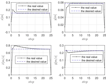
is analyzed here. The step length S and step width D are 0.4 m and 0.2 m respectively, and the height of the CoM z is 1 m. The desired step duration is set to be 0.6 s. Disturbance imposed on the initial state for the simulation is taken as ex = 10−3 m, ey = 10−3 m. The
2.5. Transition based on time 0.2 0.4 0.6 0.8 1 T 0 5 10 15 20 25 eigenvalues kS =kD = 0 1 λ1 λ2 λ3 λ4 0.2 0.4 0.6 0.8 1 T 0 5 10 15 20 25 kS = 1, kD = 1 1 λ1 λ2 λ3 λ4
Figure 2.7 – Values of the four eigenvalues for different step durations T when transition is based on time.
eigenvalues calculated for the linearized restricted Poincaré map are: |λ1| = |λ2| = 0,
|λ3| = |λ4| = 2.497.
(2.37)
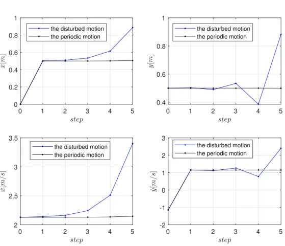
The stance foot position and the CoM evolution for both periodic and disturbed motions are illustrated in Figure 2.8, while the state evolutions are illustrated in Figure 2.9. The periodic motion is represented with the black curves and lines while the disturbed motion represented with the blue curves and lines in Figures 2.8 and 2.9. It can be seen clearly that the CoM position diverges quickly when disturbances exist. In this case, the effect of instability is that the walking is not along the expected path (here along x axis) but the direction of walking is perturbed along right or left direction depending on the perturbation. This kind of motion is often observed on the humanoid robots as Nao for example.
In consequence, this kind of control is not naturally synchronized and a high-level control must be added to produce a synchronized or stable walking gait. In the following sections, we will prove that by defining proper virtual constraints and a phasing variable depending on the state of the robot, self-synchronization and self-stabilization of the walking gait can be obtained.
-1 0 1 2 3 4 5 0 0.2 0.4 0.6 0.8 1
1.2 the periodic motion
the disturbed motion
Figure 2.8 – Evolution of CoM of the LIP model when transition is based on time with
kS = kD = 0 for 5 steps. The black and blue circles represent the stance feet and the
2.5. Transition based on time 0 1 2 3 4 5 0 0.2 0.4 0.6 0.8 1
the disturbed motion the periodic motion
0 1 2 3 4 5
0.4 0.6 0.8 1
the disturbed motion the periodic motion
0 1 2 3 4 5
2 2.5 3 3.5
the disturbed motion the periodic motion
0 1 2 3 4 5 -2 -1 0 1 2 3
the disturbed motion the periodic motion
Figure 2.9 – Evolution of the states of the LIP model when transition is based on time for kS = kD = 0 for 5 steps.
Figure 2.10 – The step finishes when the CoM crosses the switching manifold. The dashed line is the periodic motion of the CoM, and the solid line the CoM motion under an initial position perturbation.
2.6
Transition based on the horizontal CoM position
2.6.1
The virtual constraints
The vertical trajectory of the swing foot is defined as a function of a phasing variable based on the horizontal CoM position Φ(X, Y ). The transition happens when the swing foot touches the ground, which defines a relationship between the two variables X and Y . An infinite number of CoM positions satisfy it. This set of positions are grouped in the switching configuration manifold defined by:
S = {(X, Y )|zs(Φ) = 0}. (2.38)
There will be infinite sets of positions of the CoM that satisfy this condition. In this chapter, we choose a phasing variable such that the robot switches its stance leg when the CoM crosses the switching manifold defined by
S = {(X, Y )|(X − X∗−) + C(Y − Y∗−) = 0}. (2.39)
The switching manifold S is defined as a line parameterized by C, represented by the red line in Figure 2.10. Many other sets of positions can be considered but since stability studied here is a local property, a straight line is a convenient choice. The choice of S directly affects the final CoM position for a step.