Bootstrapping high frequency data
Texte intégral
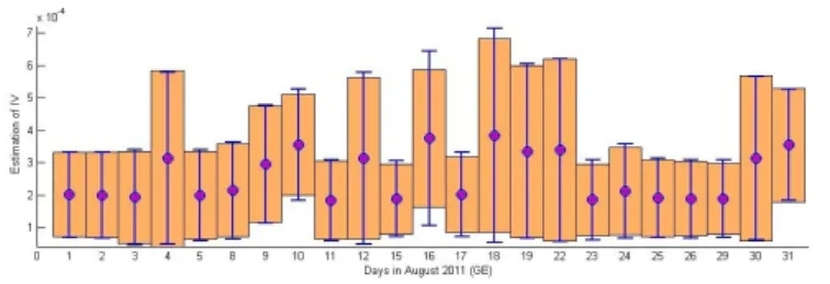
Figure
Documents relatifs
La comparaison de l’effet des différents niveaux de température sur le taux de chlorophylle chez les feuilles de la première vague de croissance des semis de chêne
giving in MS/MS a twin fragment of m/z 290/292 characteristic of the loss of a carboxylate group (not located on the C1 carbon atom), together with the presence of
In future work, we will investigate the meaning of the fracture normal diffusion-dispersion coefficient D Γ n in the new transmission conditions (9 9 ) of the new reduced model
P (Personne) Personnes âgées Personnes âgées Aged Aged : 65+ years Aged Patient atteint d’arthrose Arthrose Osteoarthritis Arthrosis I (intervention) Toucher
Unit´e de recherche INRIA Rennes, Irisa, Campus universitaire de Beaulieu, 35042 RENNES Cedex Unit´e de recherche INRIA Rh ˆone-Alpes, 655, avenue de l’Europe, 38330 MONTBONNOT
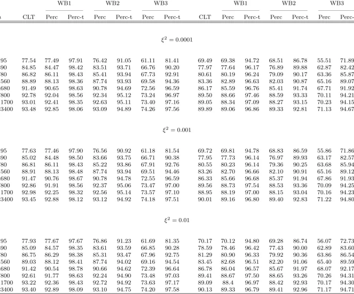
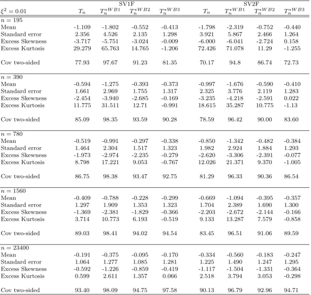
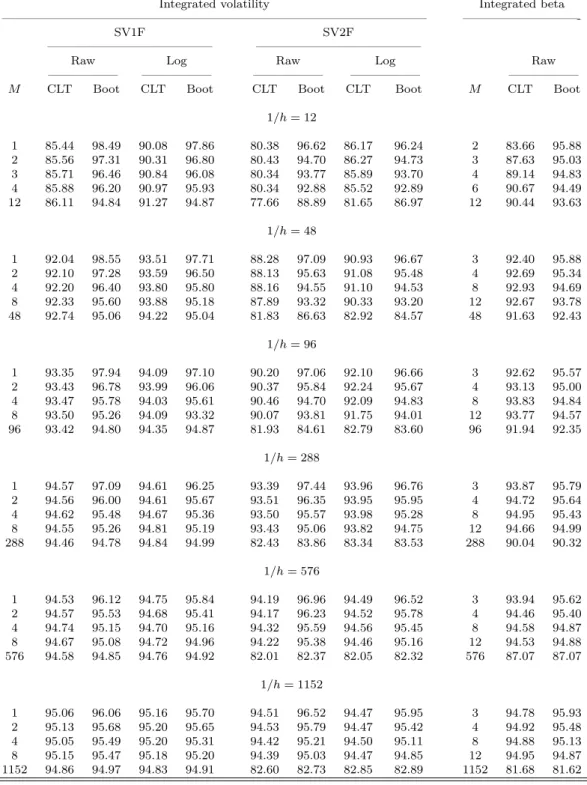
In particular given n the number of observations, the choice of N = n/2 Fourier coefficients to estimate the integrated volatility is optimal and in this case, the variance is the
When forecasting stock market volatility with a standard volatility method (GARCH), it is common that the forecast evaluation criteria often suggests that the realized volatility
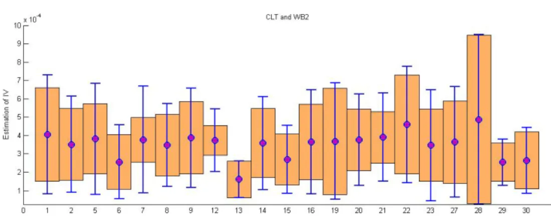
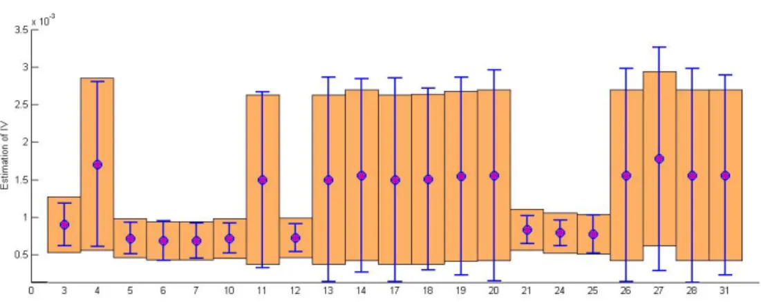
These results thus provide further evidence in favor of a warning against trying to estimate integrated volatility with data sampled at a very high frequency, when using
