NOTES D’ÉTUDES
ET DE RECHERCHE
EURO MONEY MARKET INTEREST RATES DYNAMICS
AND VOLATILITY:
How they respond to recent changes in the
operational framework
Caroline Jardet and Gaëlle Le Fol
May 2007 NER - E # 167
DIRECTION GÉNÉRALE DES ÉTUDES ET DES RELATIONS INTERNATIONALES
DIRECTION DE LA RECHERCHE
EURO MONEY MARKET INTEREST RATES DYNAMICS
AND VOLATILITY:
How they respond to recent changes in the
operational framework
Caroline Jardet and Gaëlle Le Fol
May 2007 NER - E # 167
Les Notes d'Études et de Recherche reflètent les idées personnelles de leurs auteurs et n'expriment pas nécessairement la position de la Banque de France. Ce document est disponible sur le site internet de la Banque de France « www.banque-france.fr ».
Working Papers reflect the opinions of the authors and do not necessarily express the views of the Banque de France. This document is available on the Banque de France Website “www.banque-france.fr”.
Euro money market interest rates dynamics
and volatility:
How they respond to recent changes in the operational
framework
Caroline JARDET
∗†Banque de France
Ga¨elle LE FOL
Universit´e d’Evry and CREST
March 2007
∗Corresponding author. Caroline Jardet , Banque de France, DGEI-RECFIN, UA
411391, 31 rue croix des petits champs, 75049 Paris cedex 01 00 33 (1) 42 92 49 80 [email protected].
†We thank Natacha Valla for valuable comments as well as the participants in an
internal seminar at the Banque de France. A special thanks to Stefano Nardelli for useful suggestions and for providing us data.
R´esum´e
En mars 2004, l’Eurosyst`eme a mis en place diff´erentes modifications de son cadre op´erationnel et de sa gestion de la liquidit´e. L’objectif de cet article est d’´etudier les effets de ces changements sur le niveau et la volatilit´e de l’´ecart entre l’Eonia et le taux de soumission minimum. Nos r´esultats mon-trent que ces changements ont globalement eu un effet positif sur le niveau et la volatilit´e du spread. La baisse de la volatilit´e observ´ee apr`es 2004 est largement expliqu´ee par ces modifications.
Classification JEL : E52, E58, E43
Mots cl´es : March´e mon´etaire europ´een, cadre op´erationnel, effet de liq-uidit´e.
Abstract
At the beginning of 2004, the Eurosystem implemented several modifications of its operational framework and liquidity management aiming at enhancing market efficiency. The purpose of this article is to study the effects of theses changes in the spread between the Eonia and the minimum bid rate. Our results reflect that both the operational changes as well as the new liquidity management are responsible for a significant decrease in the interest rate volatility.
JEL Classification: E52, E58, E43
Keywords: European money market, Eonia, Operational framework, Liq-uidity effect.
R´esum´e non technique
En mars 2004, l’Eurosyst`eme a mis en place diff´erentes mesures, modifi-cation du cadre op´erationnel, allomodifi-cations de liquidit´es sup´erieures au ”bench-mark” (”loose policy”) plus fr´equentes, visant `a am´eliorer la stabilit´e et l’efficacit´e du march´e mon´etaire europ´een. L’objectif de cet article est d’´etu-dier l’impact de ces changements sur le spread entre l’Eonia et le taux de soumission minimum, en niveau et en volatilit´e. Dans un premier temps, l’accent est mis sur les cons´equences du changement de cadre op´erationnel. Depuis mars 2004, la maturit´e des op´erations principales de refinancement (OPR) a ´et´e r´eduite de deux semaines `a une semaine. De plus la p´eriode de constitution des r´eserves d´ebute d´esormais le jour de r´eglement de la premi`ere OPR suivant le conseil des Gouverneurs au cours duquel sont d´ecid´es les taux directeurs. Le risque associ´e `a ce changement est de voir apparaˆıtre une plus forte volatilit´e en fin de p´eriode de constitution des r´eserves, car dans ce nou-veau cadre, le d´elai entre la derni`ere OPR et le dernier de jour de la p´eriode de maintenance (8 jours) est toujours sup´erieur `a celui observ´e avant 2004. Pour limiter cela, la fr´equence d’op´erations de r´eglages fins (FTO1
) conduites le dernier jour de la p´eriode de maintenance, a ´et´e augment´ee. Dans un second temps, nous cherchons `a ´evaluer les cons´equences de la politique de gestion de la liquidit´e mise en place par la BCE sur la p´eriode r´ecente.
Nos conclusions sont les suivantes. Les changements op´er´es au niveau du cadre op´erationnel ont globalement eu un effet positif sur le niveau et la volatilit´e du spread. La baisse de la volatilit´e observ´ee apr`es 2004 est large-ment expliqu´ee par ce changelarge-ment. Nous estimons bien une hausse de la volatilit´e le dernier jour de la p´eriode de maintenance apr`es 2004. Cepen-dant, cette hausse est bien compens´ee par la mise en place de fa¸con quasi syst´ematique de FTOs le dernier jour de la p´eriode de maintenance. En moyenne, la volatilit´e enregistr´ee `a la fin de la p´eriode de maintenance reste la mˆeme. Par ailleurs, nos r´esultats montrent que la ”loose policy” est plus efficace lorsqu’elle est men´ee `a la fin de la p´eriode de maintenance, et reduit l’´ecart entre l’Eonia et le taux de soumission minimal. De plus, la ”loose policy” a tendance `a engendrer une hausse de la volatilit´e avant 2004, alors qu’elle n’a aucun effet sur la volatilit´e apr`es 2004. Ce r´esultat peut s’expliquer par une meilleure politique de communication de la BCE apr`es 2004, qui rend publique, en plus des r´evisions de facteurs autonomes, le montant du bench-mark pour les OPRs.
1
Non technical summary
At the beginning of 2004, the Eurosystem implemented several measures such as operational framework modifications and more frequent liquidity al-lotment above the benchmark (loose policy) during its weekly main refinanc-ing operations (MROs) aimrefinanc-ing at enhancrefinanc-ing market efficiency. The goal of this paper is to study the impact of these changes on the spread between the Eonia and the minimum bid rate (spread), dynamics and volatility. First, we investigate and provide an assessment of the consequences on the spread dynamics of the changes in the operational framework in March 2004. At this date the maturity of the weekly main refinancing operations was short-ened from two weeks to one. Furthermore, since then, reserve maintenance periods have started on the settlement day of the main refinancing operation following the Governing Council meeting at which the monthly assessment of the monetary policy stance is pre-scheduled. In the new framework, the last MRO of the maintenance period is always allotted eight days before the end of the reserve maintenance period (RMP), that is, a period longer than in the previous framework. Therefore, this could lead to a greater volatility in money market interest rates at the end of the maintenance period. To avoid this problem, the ECB started to conduct fine-tuning operations (FTO) on a more regular basis. Second, we explicitly take into account liquidity effects. Actually, in the recent period, the ECB began an allotment policy, whereby it allotted above the benchmark more frequently.
The paper reaches the following conclusions. The changes of the operational framework have an overall positive impact on both the level of the spread as well as its volatility. The decrease that can be attributed to the changes is significant and large. As regards the increased number of FTOs implemented at the end of the maintenance period, it has also played its expected role. Because the period between the last MRO and the last day of the RMP in the new framework is now longer, the spread volatility should have drop-up at the end of the period. Our results show that this effects exists but is offset by the FTOs. Our results suggest that the implementation of ”loose policy” on last days of the RMP lowers the spread on either framework, but the impact is less pronounced after 2004. Concerning volatility, the ”positive” effect of pre-2004 changes does not longer exist. However, this cannot be attributed to the only operational changes. In fact, before 2004, any deviation between the MRO allotment and the benchmark amounts that banks had calculated, could be due to ECB deliberately pursuing a non-neutral liquidity target, or autonomous factors predictions errors. In the new framework, the ECB decided to also publish its calculation of the benchmark in order to avoid misperceptions in the market. Our estimation indicates that this additional
communication by the ECB has well reached its goal given that the volatility remains unchanged when a ”loose policy” is conducted.
1
Introduction
Nowadays, most central banks aim at steering a short term interest rate. This operational target is in many cases an overnight interest rate, as it plays crucial role in the financial structure, notably because it anchors the term structure of interest rates.
In the case of the Eurosystem there is no explicit target rate, as the federal fund target rate in the United states. Instead, the ECB provides a signalling rate, that is the minimum bid rate on its main refinancing operations. The reference for the operational overnight rate is the Eonia (Euro OverNight Index Average), which is related to the unsecured segment of the euro money market. Therefore, steering interest rate in the case of the Eurosystem means stabilizing the Eonia around the minimum bid rate.
At the beginning of 2004, the euro money market has experienced im-portant changes aiming at enhancing market efficiency. To do this, the Eurosystem implemented several measures such as operational framework modifications and more frequent liquidity allotment above the benchmark (loose policy) during its weekly main refinancing operations (MROs).
The goal of this paper is to study the impact of this operational changes on the spread between the Eonia and the minimum bid rate, hereafter the Eonia spread, dynamics and volatility. More precisely, we want to know if the observed decrease in the spread volatility is more likely to be explained by the stability of the key policy rates or by the operational and/or the liquidity management changes.
The interest for the money market and even for the European money mar-ket is not new. A great deal of research has focused on the features of the overnight interest rate, aiming to explain what drives its level and volatility and what factors make it diverge from the target rate. The empirical liter-ature on the conditional volatility of the overnight rate was initiated by the seminal article by Hamilton (1996). While that paper has a strong focus on testing the martingale hypothesis for the federal fund rate, it also analyses the calendar as well as the reserve maintenance period (RMP) effects on the overnight interest rate volatility in a EGARCH framework. Since then, this specification has been widely used in the literature on interbank rates. See for example, P´erez-Qu´ıros and Rodr´ıguez-Mendizabal (2005) for an applica-tion to German and European overnight rates. Gaspar, P´erez-Qu´ıros and Sicilia (2001) use a similar model to analyze the individual rates reported by the banks contained in the Eonia panel. Bartolini, Bertola and Prati (2002) analyze the volatility in daily overnight rates for a whole set of countries, including the euro area. These articles confirm the existence of empirical
regularities in the mean and the volatility of the overnight rate dynamics. Some are usual seasonal patterns known as end of period effects (end of week, end of month, end of quarter...). Other regularities can be associated with the operational framework of monetary policy. More specifically the volatility of the overnight interbank rate tends to be higher at the end of the reserve maintenance period. As regards volatility transmission, conclusions are more heterogeneous. Ayuso and al (1997) estimate the volatility of the money market rates for various European countries before European Mone-tary Union (EMU). They use an EGARCH model and introduce an estimate of the overnight rate volatility as exogenous variable. Their study leads to the conclusion of a significant volatility transmission from overnight to longer-term money market rates. While this transmission is rejected on UK data (Vila Wetherit (2003)), it is confirmed on post-EMU data at least for shorter maturities (Cassola and Morana (2006), Alonso and Blanco (2005), Durr´e and Nardelli (2006)).
Another strand of the literature has tried to improve the specification of the mean equation of the overnight rate, distinguishing between short run and long run dynamics, or emphasizing asymmetries and non-linearities. W¨urtz (2003) estimates a non linear equation for the spread between Eonia and the official rate in order to take into account that the Eonia is bounded by the corridor set by European Central Bank’s (ECB) standing facilities. Sarno and Thornton (2003) estimate non-linear error-correction equations for the US Federal Funds rate and the three-month Treasury bill rate. They find that the adjustment of the overnight rate to the Treasury bill is asymmetric. Kuo and Enders (2004) and Clarida and al. (2006) show that non-symmetric error correction is also present in the Japanese and the German term structure. Nautz and Offermanns (2005) investigate the dynamic adjustment of the Eonia to the term spread and the ECB’s policy rate. They show that the adjustment of the Eonia is significantly stronger when the policy spread is below average. This result is also present in the study of Ayuso and Repullo (2003). According to these authors, this asymmetry in the Eonia dynamics comes from the fact that the central bank is more averse to let interest rate fall below the target than let them exceed it (asymmetric loss function).
The present paper is in line with previous studies. Indeed, we use the EGARCH specification to model the Eonia spread. However, this paper differs from existing literature in the followings ways.
First, we investigate and provide an assessment of the consequences on the spread dynamics of the changes in the operational framework in March 2004. At this date the maturity of the weekly main refinancing operations (MRO) was shortened from two weeks to one. Furthermore, since then, re-serve maintenance periods have started on the settlement day of the main
refinancing operation following the Governing Council meeting at which the monthly assessment of the monetary policy stance is pre-scheduled. The ob-jective of the combined measures was to contribute stabilizing the conditions in which credit institutions bid in the MRO. However, in the new framework, the last MRO of the maintenance period is always allotted eight days before the end of the reserve maintenance period, that is, a period longer than in the previous framework. Therefore, this could lead to a greater volatility in money market interest rates at the end of the maintenance period (see Decker and Valla (2005), Durr´e and Nardelli (2006)).
Second, we explicitly take into account liquidity effects. On one hand, liquidity appears to be a natural candidate to explain interest rates dynamics as they come from the matching of demands and supplies and thus depends on the liquidity inflows. On the other hand, in the recent period, the ECB began an allotment policy, whereby it allotted above the benchmark more frequently. In fact, as mentioned in Gonzalez-Paramo (2007), ”[...] large volume in each MRO have [...] grown four-fold since the beginning of 2004. Half of this increase was caused by the shortening of the MRO maturity [...], while the other half reflects the continued expansion in the liquidity deficit”. The rest of the paper is structured as follows. Section 2 describes the Eurosystem monetary policy framework with a special focus concerning the changes of the operational framework in March 2004. Section 3 presents the data and provides some descriptive statistics and the econometric specifica-tion. In section 4, we present empirical results. The last section concludes the paper.
2
Recent changes in the operational
frame-work and liquidity policy in the
Eurosys-tem
2.1
Operational framework
In order to achieve its primary objective, the Eurosystem has a set of mon-etary instruments and procedures at its disposal. This set forms the oper-ational framework. Its main components are: the open market operations (OMOs), the standing facilities and the minimum reserve requirement.
Open market operations play an important role in steering interest rates, signalling the stance of monetary policy and managing the liquidity situation in the money market. The main refinancing operations (MROs) are the most
important open market operations. Through MROs, the Eurosystem lends funds to its counterparts against collateral with a weekly frequency. This lending normally takes place in the form of a reverse transaction. The Eu-rosystem may also carry out fine tuning operations (FTOs). The frequency and maturity of such operations are not standardized. They can be liquidity-absorbing or liquidity-providing. They aim at managing the liquidity situ-ation, in particular to smooth the effects on interest rates of unexpected liquidity fluctuations in the money market.
The Eurosystem also offers two standing facilities to its counterparts, the marginal lending facility and the deposit facility. They both have an overnight maturity and are available to counterparts on their own initiative. The corresponding interest rates provide a ceiling and a floor for the overnight rate in the money market. Therefore, by setting the rates on the standing facilities, the Governing Council determines the corridor within which the overnight money market can fluctuate.
Finally, the ECB requires credit institutions to hold deposits on accounts with the national central banks (NCBs), the ”minimum” or ”required” re-serve. On the first hand, the role of reserve requirements is to create a liquid-ity deficit. On the other hand, the averaging provision on reserve fulfilment2
tends to stabilize short term interest rates as a result of an intertemporal arbitrage mechanism.
2.2
Changes of the operational framework as of March
2004
The Eurosystem monetary policy framework has experienced periods of ten-sion in the past when pronounced speculation on an imminent interest rate change has affected counterpart’s bidding in the main refinancing opera-tions, known as ”overbidding” and ”underbidding” episodes. Both problems stemmed mainly from the fact that the timing of the reserve maintenance periods was independent of the dates of the Governing Council meetings at which changes in the key ECB rates were decided. Thus changes in the key ECB interest rate could occur within a reserve maintenance period. In addi-tion, the maturity of the weekly MROs (which was two weeks long) was such that the last operation of each reserve maintenance period overlapped with the subsequent reserve maintenance period. As a result, bidding behavior at
2
This means that compliance with reserve requirements is determined on the basis of the average of the daily balances on the counterpart’s reserve accounts over a reserve maintenance period of around one month.
the end of a maintenance period could be affected by expectations of changes in the key ECB interest rates in the next reserve maintenance period.
To respond to this problem, the Governing Council decided in 2003 on two measures, effective as of March 2004:
• Change of the timing of the maintenance period beginning. More pre-cisely, it was decided that maintenance periods would start on the set-tlement day of the first MRO following the Governing Council meeting at which the monthly assessment of the monetary policy stance was pre-scheduled. This was to ensure that there are no expectations of changes to the key ECB rates occurring during a reserve maintenance period.
• Reduction of the maturity of MROs from two weeks to one week. This aimed at eliminating the spill-over of interest rate speculation from one reserve maintenance period to the next.
The objective of the combined measures was to contribute towards stabi-lizing the conditions in which credit institutions bid in the MRO and therefore stabilizing money market volatility.
However, it was noted that some risks could be associated with these changes. For instance, as a consequence of the reduction of the MRO ma-turity, the allotment amounts of MROs would double. Therefore one could expect that some credit institutions could face difficulties to adjust their bids, especially with regard to the collateral requirements. More importantly, as regards money market volatility, it can be stressed that in the new frame-work, the last MRO of the maintenance period is one week from the end of the reserve maintenance period. Therefore, this could generate large aggre-gate liquidity imbalances at the end of the maintenance period, leading to greater volatility in money market interest rates.
2.3
The liquidity management by the Eurosystem over
the recent period
Being the monopolistic supplier of liquidity, the Eurosystem can steer short-term interest rates. Its aim is to provide the liquidity needed by the banking community, that is, the amount that helps banks to fulfill their reserve re-quirement (benchmark).
In parallel with the operational framework modifications, the Eurosystem has experienced a significant change in the liquidity management over the recent period.
This change is first materialized by more frequent FTOs at the end of the maintenance period. Actually, as noted above, one risk associated with the new framework is an increase in the likelihood of having large imbalances during the last week of a maintenance period. To avoid this problem, the ECB started to conduct fine-tuning operations on the last day of the main-tenance period on a more regular basis. Hence, we observe in our sample 8 FTOs in the old framework. Only 1 out of 8 occurred the last day of the maintenance period. In contrast, in the new framework, 22 out of 23 oc-curred the last day of the maintenance period. A higher frequency of FTOs, and particularly at the end of the maintenance period, should contribute to reduce the volatility of the Eonia spread. Consequently, in order to provide unbiased assessment of the operational framework change in the volatility of the Eonia spread, we must take into account FTOs.
In addition, the evolution of the Eonia spread under the new operational framework has showed a quite unexplained slight upward trend during the summer 2004 and autumn 2005. In reaction to that, the ECB began an allotment policy, whereby it allotted above the benchmark in all MROs, with the exception of the final operation in a maintenance period. This policy was at first successful in containing spreads. However, in spring 2006, money market spread again showed an increasing trend, and the ECB started to allot above the benchmark in the final MRO as well. As a result, in our sample, the ECB has allotted above the benchmark 320 times in the new framework, against 192 in the old one.
The risk associated with ”loose policy” was that it could be misinter-preted by market participants. In 2002, the formula for the benchmark was published. Moreover before 2004, the ECB also provided its forecasts of the average autonomous factors. However, the forecast of the benchmark was left to banks. Therefore when banks observed a deviation between the MRO allotment amount and the benchmark they had calculated, there was un-certainty about the cause of this deviation, that is a deliberate non-neutral policy of the ECB, or simple update of the autonomous factors update. In order to avoids such misunderstanding, the ECB decided to systematically provide after 2004 its forecast of autonomous factors and its calculation of the benchmark allotment amount. This additional communication in the new framework should also contribute towards stabilizing the money market volatility by reducing uncertainty in periods of loose policy.
3
Data description and descriptive statistics
3.1
Interest rate data and variables
The analysis focuses on a key money market rate of the unsecured segment, the Eonia. The Eonia is a volume-weighted average of daily interest rates reported by a panel of approximately 50 banks that have the highest business volume in the unsecured euro money market. It is computed by the ECB and published between 6.45 p.m. and 7.00 p.m.
Whereas the Eonia rates was launched with the adoption of the Euro on the first of January 1999, we choose to start our analysis on June 28, 2000. This date corresponds to the implementation of the current variable rate ten-der procedure adopted by the ECB for its main refinancing operations. The sample period runs from that date to January 16, 200 (1677 observations).
In this article, we compare the Eonia with the ”official” or ”target” mon-etary policy rate. Here, this rate is the minimum bid rate set by the ECB in the variable rate tenders applied in its weekly main refinancing operations.
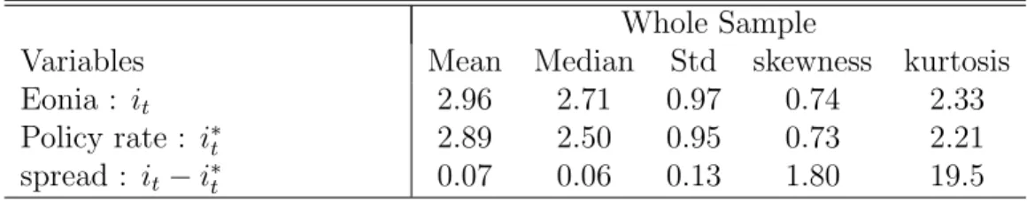
Whole Sample
Variables Mean Median Std skewness kurtosis
Eonia : it 2.96 2.71 0.97 0.74 2.33
Policy rate : i∗
t 2.89 2.50 0.95 0.73 2.21
spread : it− i∗t 0.07 0.06 0.13 1.80 19.5
Table 1 : Descriptive statistics, from June, 28 2000 to January, 16 2007 . Table 1 shows that, over the whole sample, the overnight rate is on av-erage above the official rate by around 7 bp. One factor accounting for this spread is that transactions on the unsecured money market are riskier than transactions with the ECB. In addition, we observe that standard deviations of both rates are quite similar.
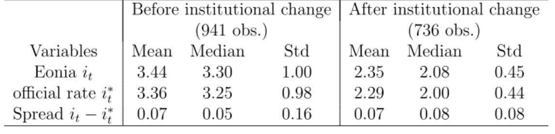
As noted above, in March 2004, two modifications have been carried out to hamper the tensions on the money market observed since the year 2000. First, the calendar of the beginning of the reserve period has been modified. Second, the duration of the main refinancing operation has been short-ened from two weeks to one. A first glance at the statistics over the two subsamples, given in table 2, can give some insight concerning the impact of such changes.
Before institutional change After institutional change
(941 obs.) (736 obs.)
Variables Mean Median Std Mean Median Std
Eonia it 3.44 3.30 1.00 2.35 2.08 0.45
official rate i∗
t 3.36 3.25 0.98 2.29 2.00 0.44
Spread it− i∗t 0.07 0.05 0.16 0.07 0.08 0.08
Table 2 : Descriptive statistics from June, 28 2000 to March 9, 2004 (Before institutional change), and from March, 10 2004 to January, 16, 2007 (After institutional change).
We note a decrease in the mean of the Eonia rate by almost 109 ba-sis points between the two sub-samples. However, this more likely reflects the drop in level of the official rate rather than the operational framework changes. In contrast, the mean of the Eonia spread is unchanged before and after 2004. The former result seems to indicate that the policy allotment have been successful in containing the upward trend of the spread experienced in the new framework.
But more important, the standard deviation of the Eonia fell by around 55 bp whereas the spread one fell by around 44 bp. Because money market volatility might give the market confusing messages about the stance of mon-etary policy, any change accompanied with a lowering of the volatility seems quite a success.
Finally, these statistics seem to indicate that monetary policy implemen-tation over the recent period has contained the spread between the Eonia and the minimum bid rate, and reduced its volatility. At least three ele-ments may explain this success : the official rate was very stable, the new operational framework is implemented, and liquidity management by ECB. The key question is to determine which of these three elements plays the most important role in explaining the change the Eonia spread.
3.2
Seasonal and microstructure dummies
We construct standard dummies to take into account calendar effects which are end-of-the-week (EOW), end-of-the-month (EOM), end-of-the-quarter (EOQ) and end-of-the-year (EOY). We also introduce other dummies to ac-count for the structure of the money market: main refinancing operation announcement and settlement (MROa and MROs, respectively), monetary policy day (MPD), namely the day on which the monthly stance of monetary policy is decided and announced, first and last days of the reserve mainte-nance period (RMP), the last week of the RMP, that is all the days between
the last MRO of the maintenance period and the last day before the end of the reserve maintenance. We also take into account in our estimation po-tential tensions caused by episodes of underbidding (relevant before march 2004), by including a dummy variable equal to one when an underbidding situation occurs.
3.3
Liquidity variable
As previously noted, over the recent period, the amount allotted at MROs has been frequently above the benchmark3
. When the spread between the allotted amount and the benchmark is positive, the liquidity conditions are targeted to be ”loose”. In this case, there is an excess of reserves in the market.
In order to take into account the ”loose policy” effects on the mean and the volatility in the new framework, we include in our explanatory variables set a dummy variable that is equal to one when a ”loose policy” is imple-mented.
We can expect that short-term interest rates will react very sensitively to changes in the aggregate liquidity supply the last week of the RMP. Ac-tually on the last days of the periods, banks can no longer postpone their fulfilment of reserve requirements and are very sensitive to the liquidity sit-uation. Therefore, the ”policy loose” variable is decomposed into a variable measuring the spread during the last MRO of the RMP (”policy loose last”) and a second one that provide the spread on the other MROs (”policy loose other”).
The recent period is also characterized by more frequent FTO at the end of the maintenance period. In order to take into account this fact, we also include in our estimation a dummy variable that is equal to one when a FTO is implemented the last day of the RMP.
3.4
The econometric specification
The above descriptive statistical analysis induces that the Eonia spread dy-namic did change with the institutional modifications in March 2004. The im-pact on the variance of this variable is clear and gives ground to the GARCH (Generalised autoregressive conditional heteroskedasticity) specification we choose.
This specification has also been used in the recent empirical literature on money market rate dynamics. Initiated by the seminal article by Hamilton
3
(1996), and widely used in this literature since, the mean and the conditional volatility of the overnight rate are estimated. The mean equation is assumed to be linear in some explanatory variables that include dummies for the end of periods (week, quarter, month or year), dummies characterizing the features of the operational framework (beginning and end of the reserve maintenance period, announcement or settlement days of MRO, announcement of the key interest rate by ECB and following days...).
The mean equation (1) for it− i∗t is modelled as an autoregressive model
with explanatory variables. More precisely, we have: it− i∗t = c +
p
X
k=1
φk(it−k− i∗t−k) + λXt+ σtνt (1)
where Xt is a set of explanatory variables that includes dummies variables
to take into account the operational framework and end of period effect. vt
is a i.i.d white noise. We assume the innovations vt to be distributed as
a Student-t, with degrees of freedom estimated to match the fat tails and concentration of small rate changes found in the data.
The volatility is assumed to follow an EGARCH (Exponential GARCH, see Nelson (1991)) representation and is related to a set of explanatory vari-ables, Vt , also including dummies. Gaspar and al. (2004), P´erez-Quir´os and
Rodr´ıguez-Mendiz´abal (2005), Bartolini and Prati (2004) have estimated this model for the euro overnight rate. These papers principally focus on the mar-tingale hypothesis of the overnight rate. Besides the usual seasonal effect, they emphasize significant effects related to the day of the reserve mainte-nance period (”institutional effects”). Our specification is in the line with these studies, and we model the conditional variance of the interest rates as an EGARCH process. This specification allows us to deal with possible non-linearities and asymmetric responses of conditional variances to negative and positive shocks. The EGARCH model we estimate is the following:
log(σ2 t) = ω + γ′Vt+ r X j=1 δjlog(σ 2 t−j) + p X i=1 αi|vt−i| + θivt−i (2)
The set of explanatory variables Vtinclude dummies variables to take into
account the operational framework and end of period effect.
Estimates of the parameters are obtained by maximum likelihood estima-tion (Marquard algorithm).
We perform a two-steps estimation procedure. First, the mean equation is estimated. The number of lags, p is determined by a back-testing pro-cedure, starting with a number of lags equal to 6. Then we check that the
residuals present no remaining autocorrelation by displaying autocorrelations and partial autocorrelations up to 25 lags and computing the Ljung-Box Q-statistics4
. For all the estimated models, we can not reject the hypothesis φ2 = ... = φn = 0. We also check that imposing these restrictions lead to
white noise residuals. Therefore the mean equation is : it− i∗t = c + φ1(it−1− i∗t−1) + λXt+ σtνt
Second, the volatility equation is estimated. The order of the EGARCH model, that is the number of lags r and p, are chosen in order maximize information criteria (AIC and Schwartz). For each model, we find that im-posing r = 1 and p = 1 provides better results. Therefore we retain an EGARCH(1,1):
log(σt2) = ω + γ′Vt+ δ1log(σ 2
t−1) + α1|vt−1| + θ1vt−1
Note that in this specification, strict stationarity of log σ2
t is equivalent
to δ1 <1.
In order to deal with the March 2004 structural break, we decompose the set of explanatory variables Xt (or Vt) in to sets of variables : the first one
gives the values of Xt (or Vt) before the 9th March 2004, and zero after ; the
second one gives the values of Xt(or Vt) after the 10th March 2004, and zero
before.
Finally, if we denote Ibef 2004 (resp. Iaf t2004) a dummy variable that takes
the values one all the days before March, 9th 2004 (all the days after March, 10th 2004) and zero after (before), the econometric specification we estimate is : it− i∗t = c + φ1(it−1− i∗t−1) + λ1XtIbef 2004+ λ2XtIaf t2004+ σtνt log(σ2 t) = ω + γ1′VtIbef 2004+ γ1′VtIaf t2004+ δ1log(σ 2 t−1) + α1|vt−1| + θ1vt−1
4
Empirical results
Tables 2 and 3 in the appendix report the estimates of the mean and volatility equations of the Eonia spread respectively. In what follows we will focus on
4
the effects of the operational framework pattern5
.
4.1
Global effects of the operational framework change
In this section, we question whether the lower volatility observed in the new framework is the result of the operational change, the stability of monetary policy rates, or both.
Recall that the rationale for the change was principally to avoid under-bidding episodes. First, we note that the coefficient of the ”underunder-bidding” dummy is significant in the volatility equation. Underbidding episodes are responsible for increasing the volatility. As no such episodes are present in the new framework, we can conclude that the change was successful in sta-bilizing the spread. However the downward sloping evolution of the interest rate over the period may also explain part of this stabilization. In fact, the probability to observe a monetary policy interest rate cut was very low. But this fact cannot alone explain the absence of underbidding after 2004. Ac-tually, monetary policy rates have also been very low and stable in the old framework from June 2003 to March 2004, but this was not sufficient to avoid two underbidding episodes during this period.
We include in our estimation a dummy variable that takes the value one for all the days before the March, 9th 2004 and zero after. This variable should capture all the changes that are not due to explanatory variables present in the model. For both the mean and the volatility this variable is not significant. Together with a white noise test of the residuals, this indicates that our set of explanatory variables is sufficient to explain the change.
Therefore, we try to determinate whether the sensibility of the level and the volatility of the spread are significantly different after the 2004 change. For that purpose, we test whether the sum of the coefficient associated with operational framework variables is significantly different before and after 2004.
As regard to the mean equation, the sum of the operational framework coefficient before 2004 is equal to -0.38. After 2004, this sum is equal to -0.08. A Wald test indicates that this difference is significant.
In the volatility equation, the sum of the operational framework coef-ficients before 2004 is equal to 10.34 (without including ”Underbidding”), whereas it equals 5.6 after 2004. A Wald test indicates that the difference
5
Calendar effects are residually linked to the operational framework, particularly in the new framework in which some operational events occur at more regular periods in the week or the month. This explains why calendar effect could be slightly differents before and after 2004.
is significantly different from zero. Therefore, the change of the operational framework has significantly reduced the volatility of the spread caused by op-erational patterns. The new opop-erational framework seems to have succeeded in reducing the uncertainty due to monetary policy action, and consequently, has well achieved its goal of stabilizing the Eonia around the minimum bid rate.
In the Following, we try to disentangle why the volatility of the spread is lower in the new framework.
4.2
Monetary policy decision in the new framework
We expect, from the operational framework change, a lower effect of market participants’ expectations regarding to the monetary policy rate. First, we note that this goal has been achieved as no more underbidding episode has been experienced since the beginning of the new framework. Another way to address this issue, is to look at how the dynamic of the spread reacts around the days of the monetary policy rates announcement and during the main refinancing operations.
Estimates of the volatility equation indicate that the volatility of the spread significantly increases the day that precedes the monetary policy day before the change. This result probably captures the effects of the mar-ket participants’ expectation on the volatility before the policy rates are announced. In contrast, after the change, no significant variation of the volatility is detected the day before the monetary policy day. In both sub-periods, the volatility increases on the monetary policy days. Finally, before 2004, the rise is immediately reversed the following day. We test whether the sum of the coefficients associated with the monetary policy day6
is sig-nificantly different before and after the change. A Wald test indicates that this difference is not significant. Hence, overall the volatility generated by the monetary policy rates announcement is not significantly different before and after 2004. However, in the new framework this increase is concentrated on one day, whereas it is more diffuse in the old framework, indicating that now the period of uncertainty is reduced.
We also check whether the volatility is significantly lower the days of the main refinancing operations since 2004. For that purpose, we compare the sum of the coefficients associated with the day of the MRO adjudication and settlement before and after 2004. The sum is equal to 0.78 and 0.89 before and after 2004 respectively. A Wald test indicates that this difference is not
6
significant. Therefore we conclude that the volatility observed during main refinancing operations (with no underbidding) is not significantly different in both sub-periods.
4.3
The last days of the reserve maintenance period in
the new framework
As previously noted, since 2004, the last MRO of the maintenance period is always allotted eight days before the end of the period. Therefore there could be a higher probability of the accumulation of large aggregate liquidity imbalances at the end of the period, leading to greater volatility in the spread. In this subsection, we try to establish whether this effect is significant.
Our estimates show that the coefficient of the last day of the RMP in the volatility equation is higher in the new framework (3.84 after 2004, 2.87 before). A Wald test indicates that this difference is significant. The week that precedes the end of the period, volatility tends to rise before and after the change. If this rise seems lower since 2004, a Wald test resjects this hypothesis.
Since 2004, more frequent FTOs have been implemented at the end of the maintenance period in order to compensate this eventual rise of the volatility. The dummy variable ”FTO the last day of a RMP” is significant and negative after 2004, whereas not significant before 2004. As a result, the more frequent FTOs conducted at the post 2004 end of the maintenance period seem to lower the spread volatility.
Finally, we test whether the combined effects, ”FTO at the end of the RMP+last days of the maintenance period”, are significantly different be-fore and after 2004. The result of the test shows that this difference is not significant. Therefore the FTOs implemented in the new framework have perfectly compensated the effects expected from a higher probability of more aggregate imbalances at the end of the maintenance period on the volatility of the spread.
4.4
The liquidity policy since 2004
In this section, we analyze the effect of the ”loose policy” implemented be-fore and after 2004. ”Loose policy” effects should be different whether it is implemented at the beginning or at the end of the maintenance period. For that reason, we include in our estimation one dummy variable that marks
”loose policy” occurring the last week of the maintenance period7
( ”loose policy last”) and another one for loose policy occurring any other day (”loose policy other”).
As regards the level of the spread (mean equation), we note that the coefficient of the variable ”loose policy last” is always significant, and neg-ative. This indicates that allotment policy reduces the spread between the Eonia and the minimum bid rate. The coefficient of the variable ”loose policy other” is not significant before 2004, and significant after. Furthermore, it is positive, indicating that when the ECB injects more liquidity than needed in the market at the beginning of the maintenance period, the spread tends to increase. This result is puzzling, as we may expect that more liquidity should lower the Eonia, and then lower the spread. A possible explanation is that when market participants observe a ”loose policy” at the beginning of the RMP, they expect that the ECB will probably allot under the benchmark at the end of the period in order to compensate this excess of liquidity and they prefer accumulate liquidity from now on.
As regards the volatility equation, the only significant coefficient concerns the ”loose policy last” variable before 2004 (0.83). It means that implemen-tation of a ”loose policy” used to increase uncertainty. Another explanation comes from the fact that allotments above the benchmark were rather scarce before 2004, and often conducted in response to underbidding, i.e in a hight volatility period. In addition, before 2004, when credit institution observed a deviation between the MRO allotment amount and the benchmark amount that they had calculated, they didn’t known whether the deviation was ac-tually due to the ECB deliberately pursuing a non-neutral liquidity target, or whether the autonomous factors predictions were false. In the new frame-work, the ECB decided to also publish its calculation of the benchmark in order to avoid misperceptions in the market. Our estimation indicates that this additional communication by the ECB has well reached its goal given that the volatility remains unchanged when a ”loose policy” is conducted.
5
Conclusion
The purpose of this paper was to study the effects of the ECB monetary policy framework on the Euro area money market. This paper has provided a model of the EONIA-key policy rate spread dynamics close to the well-documented analysis of the ECB operational framework on the overnight
7
The last week of the maintenance period includes all the days between the last MRO and the last day of the maintenance period.
unsecured interest rate literature. The advantage of such modelling is to allow for an inspection of the mean and volatility of the spread that includes exogenous variables.
Here, we focus on the particular changes that occurred in March 2004. The objective was to enhance the money market efficiency by stabilizing the short term interest rate around the key policy rate. The measures to achieved that goal are twofold. First, the maturity of the main refinancing operations has been shorten and the first day of the reserve maintenance periods became the settlement day of the main refinancing operation following the Govern-ing Council meetGovern-ing. Second, the Eurosystem started to perform more fine tuning operations at the end of the maintenance period and to allot regularly above the benchmark during the main refinancing operation settlement.
The paper reaches the following conclusions. The changes of the oper-ational framework have an overall positive impact on both the level of the spread as well as its volatility. The decrease that can be attributed to the changes is significant and large. Of course underbidding became less proba-ble because interest rates are non decreasing since 2004. However, the same apply to the end of 2003 period where two underbidding episodes were re-ported.
As regards monetary policy decisions, no underbidding episodes have been observed since then. Besides, the spread volatility tends to rise only on monetary policy days and not anymore on the day before. These two-days rises were compensated the following day, however the compensation was only partial.
As regards the increased number of FTOs implemented at the end of the maintenance period, it has also played its expected role. Because the period between the last MRO and the last day of the RMP in the new framework is now longer, the spread volatility should have drop-up at the end of the period. Our results show that this effects exists but is offset by the FTOs.
Finally, the ”loose policy” measure seems less convincing eventhough it seems that the ECB continue to increase the use of such practices. Our re-sults suggest that the implementation of ”loose policy” on last days of the RMP lowers the spread on either framework, but the impact is less pro-nounced after 2004. On other days, it even enlarges the spread in the new scheme. Concerning volatility, the ”positive” effect of pre-2004 changes does no longer exists. However, this cannot be attributed to the only operational changes. In fact, before 2004, any deviation between the MRO allotment and the benchmark amounts that they had calculated, could be due to ECB deliberately pursuing a non-neutral liquidity target, or autonomous factors predictions errors. In the new framework, the ECB decided to also publish its calculation of the benchmark in order to avoid misperceptions in the
mar-ket. This study allows for a better understanding of the impact of the 2004 changes as a all. It pointed out that the very low and stable level of short term interest rate are in favour of the new operational framework. One way to test the robustness of these results is to run the same estimation in a similar decreasing interest rate period. Another way to adress this issue is to analyse the impact of bull/bear market anticipations.
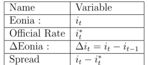
Appendix
Name Variable Eonia : it Official Rate i∗ t ∆Eonia : ∆it= it− it−1 Spread it− i∗tMean equation Variables Coefficients Constant 0.016*** (0.004) Before march 2004 -0.003 (0.007) it−1− i∗ t−1 0.622*** (0.053) Before 2004 After 2004
Last day of the week 0.01 -0.005
(0.011) (0.003) Two last days preceding the end of 0.055 0.001
the month (0.006) (0.002)
End of the month 0.050*** 0.020***
(0.011) (0.005) Two days preceding the end of the 0.007 0.016
quarter (0.010) (0.010)
End of the quarter 0.140*** 0.040*** (0.046) (0.015) Two days preceding the last day of 0.003 -0.004
the year (0.026) (0.014)
End of the year 0.043 0.021
(0.061) (0.023) Table 2 : Mean equation.
standard deviation are indicated in the brackets.
Mean equation (continued)
Day of MRO adjudication 0.008 0.001 (0.010) (0.002) Day of MRO settlement -0.004 0.002
(0.012) (0.007)
Last week of the RMP 0.030 0.030
(0.023) (0.024)
Last day of the RMP -0.070 0.121
(0.043) (0.078) FTO the last day of RMP -0.349*** -0.152* (0.042) (0.082) Two first days of the RMP 0.042** 0.011
(0.020) (0.014)
Monetary policy day 0.032 -0.059
(0.019) (0.033) Two days following the monetary 0.010 -0.031
policy day (0.011) (0.034)
Underbidding 0.100
(0.092)
Loose policy last week of the RMP -0.163*** -0.029* (0.044) (0.017) Loose policy other days of the RMP 0.011 0.018***
(0.008) (0.006) Table 2 (continued) : Mean equation.
standard deviation are indicated in brackets.
Volatility equation Variables Coefficients Constant -3.430*** (0.274) Before march 2004 0,283 (0.193) |νt−1| 0.839*** (0.059) νt−1 0.122*** (0.038) log(σ2 t−1) 0.707*** (0.023) Before 2004 After 2004 Last day of the week 0.571*** 0.158
(0.205) (0.294) Two last days preceding the end of -0.663*** 0.046
the month (0.209) (0.279)
End of the month 1.966*** 1.048***
(0.329) (0.500) Two days preceding the end of the 0.249 0.462
quarter (0.434) (0.450)
End of the quarter 2.087*** -0.078*** (0.808) (0.913) Two days preceding the last day of 0.242 -0.041
the year (1.440) (0.839)
End of the year 0.163 1.041
(1.576) (1.313) Table 3 : Volatility equation.
standard deviation are indicated in brackets.
Volatility equation (continued)
Day of MRO adjudication 0.303* 0.119 (0.179) (0.260) Day of MRO settlement 0.486** 0.787***
(0.193) (0.254) Last week of the RMP 1.726*** 1.429***
(0.167) (0.293) Last day of the RMP -2.879*** 3.842
(0.324) (0.606) FTO the last day of RMP 0.728 -1.100* (1.427) (0.617) Two first days of the RMP -0.245 -0.897***
(0.191) (0.193) One day before the monetary 0.517** 0.282
policy day (0.230) (0.501)
Monetary policy day 1.785 1.403*** (0.275) (0.384) Two days following the monetary -1.159 -0,180
policy day (0.276) (0,488)
Underbidding 2.592***
(0.471)
Loose policy last week of the RMP 0,835*** -0.202 (0.224) (0.169) Loose policy last week of the RMP -0.083 0.2143 (0.103) (0.112) Table 3 (continued) : Volatility equation.
standard deviation are indicated in brackets.
References
[1] Alonso F., and R. Blanco (2005): ”Is the volatility of the Eonia trans-mitted to the longer-term euro money market interest rates ?”, Working paper 0541, Banco de Espa˜na.
[2] Ayuso J., A. G. Haldane and F. Restoy (1997): ”Volatility Transmission Along the Money Market Yield Curve”, Weltwirtschaftliches Archiv, 133(1).
[3] Ayuso J. and R. Repullo (2003): ”A Model of the Open Market Op-eration of the European Central Bank”, Economic Journal, 113, pp. 883-902.
[4] Bartolini L., G. Bertola and A. Prati (2002): ”Day-to-day Monetary Policy and Volatility of Federal Funds Interest Rates”, Journal of Money, Credit and Banking, 34, pp. 137-159.
[5] Bartolini L. and A. Prati (2006): ”Cross-country differences in mone-tary policy execution and money market rates’ volatility ”, European Economic Review, 50(2), pp. 349-376.
[6] Cassola N., Ewerhart C. and N. Valla (2006): ”Optimal bidding in vari-able rate tenders with collateral requirements”, mimeo.
[7] Cassola N. and C. Morana (2003): ”Volatility of Interest Rates in the Euro Area: evidence from high frequency data”, Working paper 235, ECB.
[8] Clarida R.H., L. Sarno, M. P. Taylor and G. Valente (2006): ”The Role of Asymmetries and Regime Shifts in the Term Structure of Interest Rates”, Journal of Business, 79(3), pp. 1193-1225.
[9] Decker D. and N. Valla (2005), ”The Eurosystem’s monetary policy op-erational framework: first experience with the changes of March 2004”, working paper, ECB.
[10] Durr´e A., and S. Nardelli (2006), ”Volatility in the euro area market: Ef-fects from the monetary policy operational framework”, Working paper, ECB.
[11] ECB (2004): ”The implementation of Monetary Policy in the Euro Area. General documentation on Eurosystem monetary policy instruments and procedures”.
[12] ECB (2004): ”The Monetary Policy of the ECB”. [13] ECB (2005) : ”Euro Money Market Study 2004”.
[14] Gaspar V., G. P´erez Quir´os and H. Rodr´ıguez Mendiz´abal (2004): ”In-terest Rate Determination in the Interbank Market”, Working paper 351, ECB.
[15] Gaspar V., G. P´erez Quir´os and J. Sicilia (2001): ”The ECB Mone-tary Policy Strategy and the Money Market”, International Journal of Finance and Economics,6, pp. 325-342.
[16] Gonz`alez-P`aramo J. M. (2007): ”The Challenges ti Liquidity Manage-ment in the Euro Area: the perspective of the ECB”, Speech at the 30th Annual European Treasury Symposium, Berlin, 25 January 2007. [17] Hamilton J. (1996): ”The Daily Market for Federal Funds”, Journal of
Political Economy, 104(1), pp. 26-56.
[18] Hartmann P., M. Manna and A. Manzanares (2001): ”The microstruc-ture of the euro money market”, Working paper, ECB.
[19] Johansen S. (1988): ”Statistical analysis of cointegration vectors”. Jour-nal of Economic Dynamics and Control, 12, pp.31-254.
[20] Johansen S. (1995): ”Likelihood-based inference in cointegrated vector-autoregressions” in Advanced Texts in Econometrics, Oxford: Oxford University Press.
[21] Johansen S. and K. Juselius (1990): ”Maximum Likelihood Estimation and Inference on Cointegration - With Applications to the Demand for Money”, Oxford Bulletin of Economics and Statistics, 52(2), pp. 169-210.
[22] Kuo S.-H. and W. Enders (2004): The Term Structure of Japanese Inter-est Rates: the equilibrium spread with asymmetric dynamics”. Journal of the Japanese and International Economics, 18, pp. 84-98.
[23] Nautz D. and C. J. Offermanns (2005): ”The Dynamic Relationship Between the Euro Overnight Rate, the ECB’s Policy Rate and Term Spread”, Working paper, Goethe University Frankfurt.
[24] Nelson D. B. (1991): ”Conditional heteroskedasticity in asset returns: a new approach”, Econometrica, 59, pp. 347–370
[25] P´erez-Quir´os G. and H. Rodr´ıguez-Mendiz´abal (2006): ”The Daily Mar-ket for Funds in Europe: has something changed with the EMU?”, Jour-nal of Money, Credit and Banking, 38(1), pp. 91-110.
[26] Pfeiffer M. (2004): ”Measures to Improve the Efficiency of the Opera-tional Framework for Monetary Policy”, Monetary Policy and the Econ-omy Q3/04, pp. 22-33.
[27] Prati A. L. Bartolini and G. Bertola (2003): ”The Overnight Interbank Market: evidence from the G-7 and the euro zone”, Journal of Banking anf Finance, 27, pp. 2045-2083.
[28] Sarno L. and D. L. Thornton (2003): ”The Dynamic Relationship be-tween the Federal Funds Rate and the Treasury Bill Rate: an empirical investigation”, Journal of Banking and Finance, 27, pp.1079-1110. [29] Vila Wetherilt A. (2003) :”Money market operations and short-term
interest rate volatility in the United Kingdom”, Applied Financial Eco-nomics, 13(10), pp. 701-719.
[30] W¨urtz F. R. (2003): ”A Comprehensive Model of the Euro Overnight Rate”, Working paper 207, ECB.
Notes d'Études et de Recherche
1. C. Huang and H. Pagès, “Optimal Consumption and Portfolio Policies with an Infinite Horizon: Existence and Convergence,” May 1990.
2. C. Bordes, « Variabilité de la vitesse et volatilité de la croissance monétaire : le cas français », février 1989.
3. C. Bordes, M. Driscoll and A. Sauviat, “Interpreting the Money-Output Correlation: Money-Real or Real-Real?,” May 1989.
4. C. Bordes, D. Goyeau et A. Sauviat, « Taux d'intérêt, marge et rentabilité bancaires : le cas des pays de l'OCDE », mai 1989.
5. B. Bensaid, S. Federbusch et R. Gary-Bobo, « Sur quelques propriétés stratégiques de l’intéressement des salariés dans l'industrie », juin 1989.
6. O. De Bandt, « L'identification des chocs monétaires et financiers en France : une étude empirique », juin 1990.
7. M. Boutillier et S. Dérangère, « Le taux de crédit accordé aux entreprises françaises : coûts opératoires des banques et prime de risque de défaut », juin 1990.
8. M. Boutillier and B. Cabrillac, “Foreign Exchange Markets: Efficiency and Hierarchy,” October 1990.
9. O. De Bandt et P. Jacquinot, « Les choix de financement des entreprises en France : une modélisation économétrique », octobre 1990 (English version also available on request). 10. B. Bensaid and R. Gary-Bobo, “On Renegotiation of Profit-Sharing Contracts in Industry,”
July 1989 (English version of NER n° 5).
11. P. G. Garella and Y. Richelle, “Cartel Formation and the Selection of Firms,” December 1990.
12. H. Pagès and H. He, “Consumption and Portfolio Decisions with Labor Income and Borrowing Constraints,” August 1990.
13. P. Sicsic, « Le franc Poincaré a-t-il été délibérément sous-évalué ? », octobre 1991.
14. B. Bensaid and R. Gary-Bobo, “On the Commitment Value of Contracts under Renegotiation Constraints,” January 1990 revised November 1990.
15. B. Bensaid, J.-P. Lesne, H. Pagès and J. Scheinkman, “Derivative Asset Pricing with Transaction Costs,” May 1991 revised November 1991.
16. C. Monticelli and M.-O. Strauss-Kahn, “European Integration and the Demand for Broad Money,” December 1991.
17. J. Henry and M. Phelipot, “The High and Low-Risk Asset Demand of French Households: A Multivariate Analysis,” November 1991 revised June 1992.
19. A. de Palma and M. Uctum, “Financial Intermediation under Financial Integration and Deregulation,” September 1992.
20. A. de Palma, L. Leruth and P. Régibeau, “Partial Compatibility with Network Externalities and Double Purchase,” August 1992.
21. A. Frachot, D. Janci and V. Lacoste, “Factor Analysis of the Term Structure: a Probabilistic Approach,” November 1992.
22. P. Sicsic et B. Villeneuve, « L'afflux d'or en France de 1928 à 1934 », janvier 1993.
23. M. Jeanblanc-Picqué and R. Avesani, “Impulse Control Method and Exchange Rate,” September 1993.
24. A. Frachot and J.-P. Lesne, “Expectations Hypothesis and Stochastic Volatilities,” July 1993 revised September 1993.
25. B. Bensaid and A. de Palma, “Spatial Multiproduct Oligopoly,” February 1993 revised October 1994.
26. A. de Palma and R. Gary-Bobo, “Credit Contraction in a Model of the Banking Industry,” October 1994.
27. P. Jacquinot et F. Mihoubi, « Dynamique et hétérogénéité de l'emploi en déséquilibre », septembre 1995.
28. G. Salmat, « Le retournement conjoncturel de 1992 et 1993 en France : une modélisation VAR », octobre 1994.
29. J. Henry and J. Weidmann, “Asymmetry in the EMS Revisited: Evidence from the Causality Analysis of Daily Eurorates,” February 1994 revised October 1994.
30. O. De Bandt, “Competition Among Financial Intermediaries and the Risk of Contagious Failures,” September 1994 revised January 1995.
31. B. Bensaid et A. de Palma, « Politique monétaire et concurrence bancaire », janvier 1994 révisé en septembre 1995.
32. F. Rosenwald, « Coût du crédit et montant des prêts : une interprétation en terme de canal large du crédit », septembre 1995.
33. G. Cette et S. Mahfouz, « Le partage primaire du revenu : constat descriptif sur longue période », décembre 1995.
34. H. Pagès, “Is there a Premium for Currencies Correlated with Volatility? Some Evidence from Risk Reversals,” January 1996.
35. E. Jondeau and R. Ricart, “The Expectations Theory: Tests on French, German and American Euro-rates,” June 1996.
36. B. Bensaid et O. De Bandt, « Les stratégies “stop-loss” : théorie et application au Contrat Notionnel du Matif », juin 1996.
38. Banque de France - CEPREMAP - Direction de la Prévision - Erasme - INSEE - OFCE, « Structures et propriétés de cinq modèles macroéconomiques français », juin 1996.
39. F. Rosenwald, « L'influence des montants émis sur le taux des certificats de dépôts », octobre 1996.
40. L. Baumel, « Les crédits mis en place par les banques AFB de 1978 à 1992 : une évaluation des montants et des durées initiales », novembre 1996.
41. G. Cette et E. Kremp, « Le passage à une assiette valeur ajoutée pour les cotisations sociales : Une caractérisation des entreprises non financières “gagnantes” et “perdantes” », novembre 1996.
42. S. Avouyi-Dovi, E. Jondeau et C. Lai Tong, « Effets “volume”, volatilité et transmissions internationales sur les marchés boursiers dans le G5 », avril 1997.
43. E. Jondeau et R. Ricart, « Le contenu en information de la pente des taux : Application au cas des titres publics français », juin 1997.
44. B. Bensaid et M. Boutillier, « Le contrat notionnel : efficience et efficacité », juillet 1997. 45. E. Jondeau et R. Ricart, « La théorie des anticipations de la structure par terme : test à partir
des titres publics français », septembre 1997.
46. E. Jondeau, « Représentation VAR et test de la théorie des anticipations de la structure par terme », septembre 1997.
47. E. Jondeau et M. Rockinger, « Estimation et interprétation des densités neutres au risque : Une comparaison de méthodes », octobre 1997.
48. L. Baumel et P. Sevestre, « La relation entre le taux de crédits et le coût des ressources bancaires. Modélisation et estimation sur données individuelles de banques », octobre 1997. 49. P. Sevestre, “On the Use of Banks Balance Sheet Data in Loan Market Studies : A Note,”
October 1997.
50. P.-C. Hautcoeur and P. Sicsic, “Threat of a Capital Levy, Expected Devaluation and Interest Rates in France during the Interwar Period,” January 1998.
51. P. Jacquinot, « L’inflation sous-jacente à partir d’une approche structurelle des VAR : une application à la France, à l’Allemagne et au Royaume-Uni », janvier 1998.
52. C. Bruneau et O. De Bandt, « La modélisation VAR structurel : application à la politique monétaire en France », janvier 1998.
53. C. Bruneau and E. Jondeau, “Long-Run Causality, with an Application to International Links between Long-Term Interest Rates,” June 1998.
54. S. Coutant, E. Jondeau and M. Rockinger, “Reading Interest Rate and Bond Futures Options’ Smiles: How PIBOR and Notional Operators Appreciated the 1997 French Snap Election,” June 1998.
56. E. Jondeau and M. Rockinger, “Estimating Gram-Charlier Expansions with Positivity Constraints,” January 1999.
57. S. Avouyi-Dovi and E. Jondeau, “Interest Rate Transmission and Volatility Transmission along the Yield Curve,” January 1999.
58. S. Avouyi-Dovi et E. Jondeau, « La modélisation de la volatilité des bourses asiatiques », janvier 1999.
59. E. Jondeau, « La mesure du ratio rendement-risque à partir du marché des euro-devises », janvier 1999.
60. C. Bruneau and O. De Bandt, “Fiscal Policy in the Transition to Monetary Union: A Structural VAR Model,” January 1999.
61. E. Jondeau and R. Ricart, “The Information Content of the French and German Government Bond Yield Curves: Why Such Differences?,” February 1999.
62. J.-B. Chatelain et P. Sevestre, « Coûts et bénéfices du passage d’une faible inflation à la stabilité des prix », février 1999.
63. D. Irac et P. Jacquinot, « L’investissement en France depuis le début des années 1980 », avril 1999.
64. F. Mihoubi, « Le partage de la valeur ajoutée en France et en Allemagne », mars 1999. 65. S. Avouyi-Dovi and E. Jondeau, “Modelling the French Swap Spread,” April 1999.
66. E. Jondeau and M. Rockinger, “The Tail Behavior of Stock Returns: Emerging Versus Mature Markets,” June 1999.
67. F. Sédillot, « La pente des taux contient-elle de l’information sur l’activité économique future ? », juin 1999.
68. E. Jondeau, H. Le Bihan et F. Sédillot, « Modélisation et prévision des indices de prix sectoriels », septembre 1999.
69. H. Le Bihan and F. Sédillot, “Implementing and Interpreting Indicators of Core Inflation: The French Case,” September 1999.
70. R. Lacroix, “Testing for Zeros in the Spectrum of an Univariate Stationary Process: Part I,” December 1999.
71. R. Lacroix, “Testing for Zeros in the Spectrum of an Univariate Stationary Process: Part II,” December 1999.
72. R. Lacroix, “Testing the Null Hypothesis of Stationarity in Fractionally Integrated Models,” December 1999.
73. F. Chesnay and E. Jondeau, “Does correlation between stock returns really increase during turbulent period?,” April 2000.
74. O. Burkart and V. Coudert, “Leading Indicators of Currency Crises in Emerging Economies,” May 2000.
76. E. Jondeau and H. Le Bihan, “Evaluating Monetary Policy Rules in Estimated Forward-Looking Models: A Comparison of US and German Monetary Policies,” October 2000. 77. E. Jondeau and M. Rockinger, “Conditional Volatility, Skewness, ans Kurtosis: Existence
and Persistence,” November 2000.
78. P. Jacquinot et F. Mihoubi, « Modèle à Anticipations Rationnelles de la COnjoncture Simulée : MARCOS », novembre 2000.
79. M. Rockinger and E. Jondeau, “Entropy Densities: With an Application to Autoregressive Conditional Skewness and Kurtosis,” January 2001.
80. B. Amable and J.-B. Chatelain, “Can Financial Infrastructures Foster Economic Development? ,” January 2001.
81. J.-B. Chatelain and J.-C. Teurlai, “Pitfalls in Investment Euler Equations,” January 2001. 82. M. Rockinger and E. Jondeau, “Conditional Dependency of Financial Series: An
Application of Copulas,” February 2001.
83. C. Florens, E. Jondeau and H. Le Bihan, “Assessing GMM Estimates of the Federal Reserve Reaction Function,” March 2001.
84. J.-B. Chatelain, “Mark-up and Capital Structure of the Firm facing Uncertainty,” June 2001. 85. B. Amable, J.-B. Chatelain and O. De Bandt, “Optimal Capacity in the Banking Sector and
Economic Growth,” June 2001.
86. E. Jondeau and H. Le Bihan, “Testing for a Forward-Looking Phillips Curve. Additional Evidence from European and US Data,” December 2001.
87. G. Cette, J. Mairesse et Y. Kocoglu, « Croissance économique et diffusion des TIC : le cas de la France sur longue période (1980-2000) », décembre 2001.
88. D. Irac and F. Sédillot, “Short Run Assessment of French Economic Activity Using OPTIM,” January 2002.
89. M. Baghli, C. Bouthevillain, O. de Bandt, H. Fraisse, H. Le Bihan et Ph. Rousseaux, « PIB potentiel et écart de PIB : quelques évaluations pour la France », juillet 2002.
90. E. Jondeau and M. Rockinger, “Asset Allocation in Transition Economies,” October 2002. 91. H. Pagès and J.A.C. Santos, “Optimal Supervisory Policies and Depositor-Preferences
Laws,” October 2002.
92. C. Loupias, F. Savignac and P. Sevestre, “Is There a Bank Lending Channel in France? Evidence from Bank Panel Data,” November 2002.
93. M. Ehrmann, L. Gambacorta, J. Martínez-Pagés, P. Sevestre and A. Worms, “Financial Systems and The Role in Monetary Policy Transmission in the Euro Area,” November 2002. 94. S. Avouyi-Dovi, D. Guégan et S. Ladoucette, « Une mesure de la persistance dans les
95. S. Avouyi-Dovi, D. Guégan et S. Ladoucette, “What is the Best Approach to Measure the Interdependence between Different Markets? ,” December 2002.
96. J.-B. Chatelain and A. Tiomo, “Investment, the Cost of Capital and Monetary Policy in the Nineties in France: A Panel Data Investigation,” December 2002.
97. J.-B. Chatelain, A. Generale, I. Hernando, U. von Kalckreuth and P. Vermeulen, “Firm Investment and Monetary Policy Transmission in the Euro Area,” December 2002.
98. J.-S. Mésonnier, « Banque centrale, taux de l’escompte et politique monétaire chez Henry Thornton (1760-1815) », décembre 2002.
99. M. Baghli, G. Cette et A. Sylvain, « Les déterminants du taux de marge en France et quelques autres grands pays industrialisés : Analyse empirique sur la période 1970-2000 », janvier 2003.
100. G. Cette and Ch. Pfister, “The Challenges of the “New Economy” for Monetary Policy,” January 2003.
101. C. Bruneau, O. De Bandt, A. Flageollet and E. Michaux, “Forecasting Inflation using Economic Indicators: the Case of France,” May 2003.
102. C. Bruneau, O. De Bandt and A. Flageollet, “Forecasting Inflation in the Euro Area,” May 2003.
103. E. Jondeau and H. Le Bihan, “ML vs GMM Estimates of Hybrid Macroeconomic Models (With an Application to the “New Phillips Curve”),” September 2003.
104. J. Matheron and T.-P. Maury, “Evaluating the Fit of Sticky Price Models,” January 2004. 105. S. Moyen and J.-G. Sahuc, “Incorporating Labour Market Frictions into an
Optimising-Based Monetary Policy Model,” January 2004.
106. M. Baghli, V. Brunhes-Lesage, O. De Bandt, H. Fraisse et J.-P. Villetelle, « MASCOTTE : Modèle d’Analyse et de préviSion de la COnjoncture TrimesTriellE », février 2004.
107. E. Jondeau and M. Rockinger, “The Bank Bias: Segmentation of French Fund Families,” February 2004.
108. E. Jondeau and M. Rockinger, “Optimal Portfolio Allocation Under Higher Moments,” February 2004.
109. C. Bordes et L. Clerc, « Stabilité des prix et stratégie de politique monétaire unique », mars 2004.
110. N. Belorgey, R. Lecat et T.-P. Maury, « Déterminants de la productivité par employé : une évaluation empirique en données de panel », avril 2004.
111. T.-P. Maury and B. Pluyaud, “The Breaks in per Capita Productivity Trends in a Number of Industrial Countries,” April 2004.
112. G. Cette, J. Mairesse and Y. Kocoglu, “ICT Diffusion and Potential Output Growth,” April 2004.