HAL Id: hal-01868866
https://hal.archives-ouvertes.fr/hal-01868866
Submitted on 6 Sep 2018
HAL is a multi-disciplinary open access
archive for the deposit and dissemination of
sci-entific research documents, whether they are
pub-lished or not. The documents may come from
teaching and research institutions in France or
L’archive ouverte pluridisciplinaire HAL, est
destinée au dépôt et à la diffusion de documents
scientifiques de niveau recherche, publiés ou non,
émanant des établissements d’enseignement et de
recherche français ou étrangers, des laboratoires
An Evidential Method for Correcting Noisy Information
in Social Network
Salma Ben Dhaou, Mouloud Kharoune, Arnaud Martin, Boutheina Ben
Yaghlane
To cite this version:
Salma Ben Dhaou, Mouloud Kharoune, Arnaud Martin, Boutheina Ben Yaghlane. An Evidential
Method for Correcting Noisy Information in Social Network. Online Social Networks and Media,
Elsevier, 2018, Volume 7, pp.30-44. �hal-01868866�
An Evidential Method for Correcting Noisy Information
in Social Network
Salma Ben Dhaoua,, Mouloud Kharouneb,, Arnaud Martinb,, Boutheina Ben Yaghlanea,
aLARODEC, ISG of Tunis bIRISA, Rennes1
Abstract
Nowadays, social networks have become an important part of our daily lives. Hence, several researchers have been interested in the study and analysis of the interactions between the entities composing this type of networks. By modeling a social network, we can assign attributes to nodes and links based on network and community structure. These attributes which may be uncertain, imprecise or even noisy, involve obtaining a non-coherent network. In order to remedy this problem, we propose, in this paper, a method that corrects the noise in the network using the theory of belief functions.
Keywords: Theory of Belief Functions, Communities, Social Networks, Attributed Networks
1. Introduction
Nowadays, the use of computer technology and Internet has become essen-tial. As a result, social networks became an important part of our daily lives. Therefore, it is interesting to study and analyze the types of relationships that exist in these networks. To do so, the study of the community structure as well
5
as the nodes and links attributes represent main characteristics that must be taken into account to analyze these networks.
Email addresses: [email protected] (Salma Ben Dhaou), [email protected] (Mouloud Kharoune),
In social network analysis [1, 2], the observed attributes of social actors are understood in terms of patterns or structures of ties among the units. These ties may be any existing relationship between units; for example friendship, material
10
transactions, etc.
Currently, if we observe any social network, we will soon realize that the entities composing this network are grouped, for example, according to a center of interest, a category of age, a preference, etc.
In his work, Santo Fortunato [3] explained that communities, also called
15
clusters or modules, represent groups of vertices which probably share common properties and/or play similar roles within the graph. He argues also that the word community itself refers to a social context. In fact, people naturally tend to form groups, within their work environment, family or friends.
In a social network, we can deal with missing or modified information. In
20
addition, the information exchanged can be often imperfect, due to the hetero-geneous nature of the sources. Therefore, it would be interesting to use a vector of values which represent the nodes and links attributes.
In the same context, many studies focus on modeling the uncertain social network. In fact, they represent an uncertain network by weighting the nodes
25
or links with values in [0, 1] to model uncertainties. Hence, it will be easier to monitor the behavior of the social network [4, 5]. In addition, as shown in [6], the use of evidential attributes, from the theory of belief functions, gives better results compared to the probabilistic ones.
The theory of belief functions offers a mathematical framework for modeling
30
uncertain and imprecise information [7]. It has been employed in different fields, such as data classification [8, 9] and social network analysis [10].
Furthermore, the theory of belief functions provides a flexible way of com-bining information collected from different sources. In the majority of cases, this combination is followed by decision-making. It also allows conflict management.
35
The aim of this paper is to show that even with noise in the network, our algorithm is able to classify the nodes in their initial clusters. In the case of a large noise, the algorithm guarantees the coherence of the information of any
network even when it is a network whose nodes and links attributes have been strongly modified.
40
In this paper, we focused on the use of a limited number of communities. In terms of scaling up, there are several strategies that can reduce complexity like the one presented in [11]. This will be the subject of future work.
This paper is structured as follows. In section 2, we remind some basic concepts of the theory of belief functions and review some community detection
45
methods as well as some other related works. Section 3 is dedicated to our contribution. Section 4 is devoted to the experimentations and finally section 5 concludes the paper.
2. Background
In this section, we start by recalling some basis of the theory of belief
func-50
tions, we use it in this paper in order to model uncertainties. Then we present some community detection methods that use both the structure and the at-tributes of the network.
2.1. Theory of Belief Functions
The theory of belief functions allows explicitly to consider the uncertainty
55
of knowledge using mathematical tools [7, 12]. It is a useful and effective way in many fields such as classification, decision making, representation of uncertain and inaccurate information, etc.
In fact, it is a suitable theory for the representation and management of imperfect knowledge. It allows to handle the uncertainty and imprecision of the
60
data sets, to combine mass functions and make decisions.
The principle of the theory of belief functions consists on the manipulation of functions defined on subsets. However, it does not represent uncertainty using sets of probability measures. These functions are called mass functions and range from 0 to 1.
Let Ω be a finite and exhaustive set whose elements are mutually exclusive, Ω is called a frame of discernment. A mass function is a mapping
m : 2Ω→ [0, 1]
such that
X X∈2Ω
mΩ(X) = 1 and mΩ(∅) = 0 (1)
The mass mΩ(X) expresses the amount of belief that is allocated to the subset X. We call X a focal element if mΩ(X) > 0.
A categorical mass function is a mass function with an unique focal element such that mΩ(A) = 1.
In this work, we used also another interesting concept which is the distance
70
of Jousselme [13]. This distance represents the degree of similarity between bodies of evidence. It is defined by:
dj(mΩ1, m Ω 2) = r 1 2(m Ω 1 − mΩ2)TJac(mΩ1 − mΩ2) (2) where the elements J ac(A, B) of Jaccards weighting matrix Jac are defined as: J ac(A, B) = 1 if A = B = ∅ |A ∩ B| |A ∪ B|, A, B ∈ 2 Ω\ ∅ (3)
We also consider the normalized conjunctive rule called the Dempster rule [14], given for two mass functions mΩ1 and mΩ2 for all X ∈ 2Ω, X 6= ∅ by:
m⊕(X) = 1 1 − k X A∩B=X mΩ1(A)m Ω 2(B) (4) where k = X A∩B=∅
mΩ1(A)mΩ2(B) is the global conflict of the combination. The Dempster combination rule reinforces the mass values of the elements on which the sources are agree. This rule is adapted when the combined mass functions are cognitively independent. In the case of dependent mass functions, one can use the mean rule given for two mass functions mΩ
X 6= ∅ by:
mΩ(X) = 1 2(m
Ω
1(X) + mΩ2(X)) (5) In order to make decision, we use the pignistic probability introduced by
75
Smets in [15] for normal mass functions by:
BetP (X) = X Y ∈2Ω,Y 6=∅
| X ∩ Y | | Y | m
Ω(Y ) (6)
2.2. Some Community Detection Methods with Graphs Structure and Attributes In this section, we introduce some community detection methods based on graph structure and attributes.
According to [16], an attributed graph Ga = (Va, Ea) can be defined as a set
80
of attributed vertices Va = {v1, . . . , vp, . . . , vq, . . . , vn} and a set of attributed edges Ea = {. . . , epq, . . .}. The edge epq connects vertices vp and vq with an attributed relation.
The presented model in [17] uses both information. In fact, an unified neigh-borhood random walk distance measure allows to measure the closeness of vertex
85
on an attributed augmented graph. Then, the authors use a k-Medoids cluster-ing method to partition the network into k clusters.
A second method presented in [18] consists on a model dedicated to detect circles that combine network structure and user profile. The authors learn for each circle, its members and the circle-specific user profile similarity metric.
90
They model the membership of a node to multiple circles in order to detect overlapping and hierarchically nested circles.
A third method presented in [19] consists on dealing with the uncertainty that occurs in the attribute values within the belief function framework in the case of clustering. In this work, the authors present a new version of decision
95
trees with the theory of belief functions to handle the case of uncertainty present only in attribute values for both construction and classification phases.
Thus, it is important to consider both information structure and attributes in order to detect the network communities. In fact, if one source of information
is missing or noisy, the other can solve the problem.
100
The works cited above [17, 18] use only a probabilistic attributes as well as the structure of the graph to do the clustering. In our previous work [6], we show that the use of evidential attributes gives better results than the probabilistic ones in the clustering.
The works cited [17, 18, 19] are interesting, but they do not assume that
net-105
work information can be noisy or perturbed. In addition, they do not consider the use of node and link attributes simultaneously to do clustering.
2.3. Other Related Works: Homophilic Behaviors in Social Networks
In addition of the presented community detection methods above, there are works that are related to our research such as the reconstruction of an initial
110
network and the propagation of labels.
In [20], the authors present a new method using the theory of belief functions that aims to detect communities on graphs after the stabilization of the label propagation process. In fact, SELP permits to propagate the labels from the labeled nodes to the unlabeled ones based on a propagation rule. The proposed
115
algorithm computes the dissimilarities between nodes based on the graph struc-ture. The main advantage of the proposed algorithm is that it can effectively use limited supervised information to guide the process of the detection.
Another interesting work presented in [21] aims to identify missing and spu-rious interactions (links connecting nodes) and to reconstruct network whose
120
properties are closer to the ’true’ underlying network. To do so, the authors focus on the family of stochastic block models. The proposed method can also guide new discoveries. In fact, if a given interaction between 2 nodes exists but with a very low reliability for the interaction, that means that the function of the interaction is very specific.
125
The method proposed in [22] aims to address the problem of reconstructing the original network and set of features given their randomized counterparts. The technique of data randomization consists of removing some of the original edges of the network in addition of new ones. Furthermore, the features can
be also randomized. In this work, the authors assume that data-randomization
130
method do not completely destroy the original dataset. For the case of features, every node is associated with k binary features. If the node has that feature, it will take 1 otherwise it will take 0.
All the works presented are interesting. However, we can not do a comparison at the experimental level since we do not consider the resolution of the same
135
problem. Indeed, the first work consider a network with few nodes having labels and aim to propagate them to the unlabled ones. In our case, we consider that all nodes and links have a prior lables. In the second research [21], the authors are interested in predicting links based on observations. In our work, we do not modify the initial structure of the network. Regarding the third work [22], the
140
authors remove links from the graph and add new ones whereas in our case, we do not modify the structure of the graph.
3. An Evidential Method for Correcting Noisy Information in Social Networks
In this section, we will introduce our proposed approach. First, we will
145
present the important notions used in this work. Then, we will explain the formalization of our method and finally, we will detail the main steps of the proposed algorithm.
3.1. Important Notions
In the networks, noisy or imperfect information can transit. Therefore, if we
150
limit ourselves to the network structure as well as the nodes and links attributes in the classification, the error rate may increase and the network information may become inconsistent.
To solve this problem, we propose a method that allows the classification of nodes in the case of a noisy network, based on the community structure as well
155
In the case of a significant noise introduced, our algorithm corrects inconsis-tent information. Thus, even if we do not find the initial network, we get a new coherent network. In this context, we present two notions used in this work:
Noise. A noisy element (i.e. a node or a link) is an element whose attribute
160
has been modified.
Consistency. A network is composed of a set of nodes belonging to communi-ties Ci and linked together by links. Two nodes connected by a link represent a triplet. Depending on the community structure of the network, a node belongs to a single community Ciwhile the link may be of different types. If it is inside
165
the community Ci, then it will be of the type ICi. However, if it connects two nodes belonging to two different communities, then it will be of type BC.
We use only one type of link representing the link between two communities (BC) in order to minimize the possible hypotheses, since the more the number of communities increases, the more the types of links connecting two communities
170
increase too.
In what follows, we will present the general idea of the proposed method.
3.2. Formalization
In this work, we consider a coherent triplet as a triplet (Vk1, Lk12, Vk2) that
satisfies one of the following possibilities:
175
• Vk1 ∈ Ci, Vk2 ∈ Ci, Lk12 ∈ ICi with i = 1, . . . N
• Vk1 ∈ Ci, Vk2 ∈ Cj, Lk12 ∈ BC with (i 6= j), and i, j = 1, . . . N
Figure 1 shows the notations for a given triplet k. It consists of two nodes (starting node, arrival node and link that connects them) having each one a mass function which shows the belonging possibilities of a node to a community
180
Ci. Nodes are connected through a link, that also has a mass function which indicates the possibilities of its label (A link can be of the type ICi if it is inside the community or BC if it connects two nodes belonging to two different communities).
Figure 1: Triplet k.
Thus, the triplet is defined as follow:
185
• Vk1 modelized with a mass function mΩN
k1
• Vk2 modelized with a mass function mΩN
k2
• Lk12 modelized with a mass function m
ΩL
k12
We remind that a categorical mass function is a mass function with an unique focal element such that mΩ(A) = 1. The representatives below represent the
190
community centers. We calculate the distances between the mass functions of the nodes and links and categorical mass functions of the representatives in order to be able to place these elements in a group.
• For the nodes: the categorical mass functions are defined by mΩN
ω (ω) = 1 with ω ∈ ΩN, i.e. mΩN
Ci (Ci) = 1, with i = 1, . . . , N . 195
• For the links: the categorical mass functions are defined by mΩL
ω (ω) = 1 with ω ∈ ΩL, i.e. mΩL
BC(BC) = 1 or m ΩL
ICi(ICi) = 1 , with i = 1, . . . , N .
The aim of the proposed approach is to correct the noise added to a net-work by considering each triplet independently of the others. To do this, our algorithm proceeds by calculating the distances between the mass functions of
200
each element of the triplet and the mass functions of the representatives of the communities. Then, it calculates the average distances of the 3 elements of the triplet and compares them with the average distances of the coherent triplets
defined initially. The algorithm then keeps the minimum average distance which gives us an idea about the type of the triplet.
205
The value of this minimum average distance is considered as a mass function from the current information of the network and is combined thereafter with the initial mass functions. Subsequently, for each node with several links, we will combine with the mean rule all the mass functions that are related to it. Finally, we will use the BetP to make a decision about the membership of a
210
node to a community and a link to a given type.
We will detail in the following the different steps of the proposed approach.
3.3. Main Steps of the Algorithm
The proposed approach is applied in 4 steps detailed below. In order to simplify the notations, we present in the following the equations used in one
215
iteration t of the algorithm. Step 1:
For each element of a triplet k, we calculate the distances between the latter and the corresponding categorical mass functions.
In the theory of belief functions, a distance is used to describe the difference
220
between two distinct sources of information. We use the distance of Jousselme which takes into account the quantification of the similarity between the focal elements using Jaccard similarity coefficients.
By calculating the distance between the mass function of a node or a link and the corresponding categorical mass functions that are “ideals”, we have an
225
idea about its belonging to a community or a kind of link. In fact, we keep the minimum distance and the decision corresponds to the categorical mass functions having the lowest distance with the mass function of the nodes or of the links. Hence, for each triplet (Vk1, Lk12, Vk2), with k = 1, . . . , M , M the number of triplets (or links) we calculate at iteration t:
230 Ck1 = arg min ω∈ΩN dJ(mΩk1N, m ΩN ω ) (7) Ck2 = arg min ω∈ΩN dJ(mΩN k2 , m ΩN ω ) (8)
Lk12is determined according to the coherent triplets by: Lk12= ICk1 if Ck1 = Ck2 BC if Ck1 6= Ck2 (9)
Table 1 shows the coherent values of a triplet for the case of a network containing 3 communities. This process of decision is given by [23].
Step 2:
For each triplet k, at the iteration t we calculate the average distance dk
235
obtained from each possible combination presented previously.
Hence, dk represents a minimal distance between the triplet k and the most possible categorical triplet. This average distance makes it possible to calculate the dissimilarity between any triplet and another coherent one defined initially. It is defined by: dk = dJ(mΩN k1 , m ΩN Ck1) + dJ(m ΩL k12, m ΩL Lk12) + dJ(m ΩN k2 , m ΩN Ck2) 3 (10)
Step 3: Knowledge Review
In this step, we will use the obtained value of the average distance dk to define a mass function, that will be combined with the initial mass functions of the nodes and links composing each triplet. Therefore, the average distance dkvalue is assigned to the focal elements that represent the types of the two nodes and the link composing the triplet k and the rest will be assigned to the ignorance. Hence, we have: mΩN k1d(Ck1) = 1 − dk mΩN k1d(ΩN) = dk (11) mΩL k12d(Lk12) = 1 − dk mΩL k12d(ΩL) = dk (12) mΩN k2d(Ck2) = 1 − dk mΩN k2d(ΩN) = dk (13)
Once the minimum average distance has been found, we know to which coherent triplet initially defined, the current triplet k is the closest. Therefore, we know what is the nature of each of its elements. Hence, we know if the link which connects the two nodes is of type ICi or BC.
240
The minimum average distance dk is an information provided by a network whose initial mass functions can be noisy. Therefore, this should be taken into account when reviewing knowledge.
Calculation of final Mass Functions
In this step, we update at the iteration t + 1 the mass functions obtained from
245
the previous step with the initial mass functions given at the iteration t by the following equations: mt+1,ΩN k1 = m t,ΩN k1 ⊕ m t,ΩN k1d (14) mt+1,ΩL k12 = m t,ΩL k12 ⊕ m t,ΩL k12d (15) mt+1,ΩN k2 = m t,ΩN k2 ⊕ m t,ΩN k2d (16) where mt,ΩN k1d , m t,ΩL k12d, m t,ΩN
k2d are given respectively by equations (11), (12) and
(13).
The combination of the mass functions derived from the minimal average
250
distance calculation and the initial generation by the Dempster rule provides a final idea of nodes and links belonging to their clusters. The Dempster rule affects the generated conflict to the focal elements and therefore we will not have a mass on the empty set.
Step 4:
255
As we treat each triplet independently of the others, we can have cases where several links start from the same node and so we have several mass functions for the same node. In order to determine an unique mass function for each node (e.g. Vk1), we combine by the mean rule (given by equation (5)), all the mass functions obtained for the given node Vk1 in step 3 (equation (15)). The choice
260
given node Vk1, with Mk1 links, we modify the mass functions by: mΩN k1 = 1 |T | X {k:Vk1∈T } mΩN k (17) where T = {(Vk0
1, Lk12, Vk2)} represents the triplets that contain the node Vk1
and mΩN
k is given by the equation (14).
Finally, we use the BetP given by equation (6) to make decision about the
265
belonging of the triplet (Vk1, Lk12, Vk2). We have at the iteration t + 1, in the
order of the triplet:
Ck1 = arg max X∈ΩN X Y ∈2ΩN,Y 6=∅ | X ∩ Y | | Y | m ΩN k1 (Y ) (18) Lk12 = arg max X∈ΩL X Y ∈2ΩL,Y 6=∅ | X ∩ Y | | Y | m ΩL k12(Y ) (19) Ck2 = arg max X∈ΩN X Y ∈2ΩN,Y 6=∅ | X ∩ Y | | Y | m ΩN k2 (Y ) (20)
Algorithm 1 shows the outline of the process followed for correcting noise in social network using evidential attributes.
The use of the Dempster combination rule makes it possible to reinforce from
270
one iteration to another the mass values of the elements on which the sources agree. Indeed, if we have a mass coming from each source on the same focal element, the combination rule of Dempster allows to increase the belief on the latter. From the fact that we will have an increase in mass functions values, there will be no change in the decision. Hence, we can confirm that the proposed
275
method is still converging to a single element by the decision process given by equations (18), (19) and (20).
4. Experimentations
We start the experiments by the generation of mass functions on the nodes and links according to the structure of the network. Indeed, for each node
280
Algorithm 1 An Evidential Approach for Correcting Noise
Require: Graph G(V, E), The set of labeled nodes, the set of labeled links Ensure: The corrected graph
t = 0 repeat
1. for each element of a triplet k, compute the distance of Jousselme between the mass function of the element and the corresponding categorical mass functions using Eqs (7), (8), (9)
2. for each triplet k, compute the minimum average distance dk by using Eq (10)
3. Define mass functions from the computed dk using the Eqs (11), (12), (13)
4. Update the mass functions using the Eqs (14),(15), (16),
5. Combine the mass functions for the same node in order to have a unique mass function by using the Eq (17)
6. Make decision about the belonging of each element of the triplet k using Eqs (18), (19), (20)
7. t = t + 1
on ΩN and we assign the highest generated value to Ci. We do the same for the links: depending on the type of the link, we generate two focal elements.
In a second step, we noised this network according to three scenarios: • Noisy Nodes Only: In this case, we have selected randomly a certain
285
number of nodes of the initial network and we have modified their mass functions by randomly generating two focal elements (ignorance and an-other element except the empty set).
• Noisy Links Only: In this case, we selected randomly a certain number of links of the initial network and we modified their mass functions by
290
randomly generating two focal elements (ignorance and another element except the empty set).
• Noisy Nodes and Noisy Links: In the latter case, we selected randomly some nodes and links of the networks. Then, we modified their mass functions.
295
After that, for each triplet we calculate the distances between the attributes of the link and the two nodes and the attributes of the representatives. As we consider different networks with N communities, the coherent triplets are defined on the basis of the community structure of the networks. That is to say, a node can belong to only one community Ci. From this hypothesis, the links
300
that we can have will be of type ICi if they are inside the community Ci, if not the links will be of type BC (if the nodes belong to two different communities). Then, we calculate the average of the distances of the elements composing the triplet based on the possibilities defined initially. Table 1 presents the possible triplets for the case of a network of 3 communities.
305
Thereafter, we keep the minimum average distance that will be combined with the initial mass functions by the Dempster rule. Here, the initial mass functions represent the mass functions before the calculation of our model is applied. For each node Vki belonging to several triplets, we will combine by the mean rule all the mass functions obtained at the end of the calculation of the
Vk1 Vk2 Lk12 C1 C1 IC1 C1 C2 BC C1 C3 BC C2 C2 IC2 C2 C1 BC C2 C3 BC C3 C3 IC3 C3 C1 BC C3 C2 BC
Table 1: Coherent Triplets For 3 Communities.
Dempster combination.
The proposed algorithm is iterative since, for several cases of noisy nodes and/or noisy links, the corrections are made only after a certain number of iterations.
The mass functions obtained at the end of each iteration represent the input
315
of the next iteration. For each iteration, we calculate the confusion matrix. We remind that a confusion matrix is a technique for summarizing the performance of a classification algorithm.
In order to know the accuracy value at each iteration for each case to be tested, we compared the result of the pignistic probability applied at the end
320
of each iteration with the initial information of the network before introducing the noise. The accuracy represents the ratio of correct predictions to total predictions made.
In order to show the efficiency of our method, we will compare the obtained results with those of the baseline. All experiments were repeated 10 times. All
325
figures represent the average of the accuracy calculated for 10 runs. In addition, the evidential approach and the probabilistic one are tested under the same conditions: The same elements randomly selected and noisy in the evidential
case are noisy during the probabilistic approach test.
In the tables presented in the following, we will present the accuracy averages
330
as well as the confidence intervals obtained from the evidential approach and the baseline for each type of experiment.
4.1. Possible Corrections
In the presence of noise, the algorithm corrects the information of the net-work as a function of the noisy elements and the coherent triplets initially
de-335
fined. In this section, we will present the possible corrections for the case of a network containing 3 communities:
One noisy node and the link and the other node are corrects. Initially we have the triplet: Vk1 ∈ C1, Lk12 ∈ IC1, Vk2 ∈ C1. Suppose that one of the nodes is modified and belongs now to C2or C3. The algorithm will detect that according
340
to the information given by the link and the other node, the modified one should be corrected. Therefore, the noisy node will be affected to C1. It is the same if we have a triplet Vk1 ∈ C2, Vk2 ∈ C2, Lk12 ∈ IC2or a triplet Vk1 ∈ C3, Vk2 ∈ C3, Lk12 ∈ IC3. The noisy node will be reassigned to its initial community.
Two noisy nodes and the link is correct. In that case, the algorithm will change
345
the nature of the link to obtain a coherent triplet. If the modified nodes be-longs to the same community, the algorithm will change the link in such a way that it will be internal to the same community. If the modified nodes belongs to different communuties, the algorithm will change the nature of the link to “Between Clusters” (BC).
350
One noisy node, one noisy link and one correct node. Suppose that initially we had, Vk1 ∈ C1, Lk12 ∈ IC1 and Vk2 ∈ C1. Vk1 was modified to belong to C2 or C3, Lk12 ∈ BC and Vk2 ∈ C1. In that case, the algorithm will not change the information of the triplet because it’s coherent. However, if we had for example Vk1 ∈ C2 or C3, Lk12 ∈ IC2 or IC3 and Vk2 ∈ C1, the algorithm will change 355
so the algorithm will have another information and can change one of the node based on that.
Two noisy nodes and noisy link. In that case, the algorithm will compute the minimal distance between the current triplet and the coherent ones defined
360
initially and then modify the information of the current triplet.
4.2. Used Networks
In this work, we performed our experiments on the real data Karate Club network and on networks generated by LFR.
• Karate Club Network: The Zachary Karate Club is a well-known real
365
social network studied by Zachary [24]. The study was carried out over a period of three years from 1970 to 1972.
In this network, we find:
– 34 nodes that represent the members of Karate Club.
– 78 pairwise links between members who are interacted outside the
370
club.
During the study a conflict arose between the administrator “John A” and instructor “Mr. Hi”, which led to the split of the club into two. Half of the members formed a new club around Mr. Hi, members from the other part found a new instructor or gave up karate.
375
• LFR: The LFR benchmark [25] is an algorithm that generates artificial networks that simulate real-world networks. The generated network has a prior known communities and it is used to compare different community detection methods.
4.3. Convergence
380
The previous presented algorithm is iterative which allows to obtain better results of the accuracy from one iteration to another. The stop criterion used is the stabilization of the value of the accuracy.
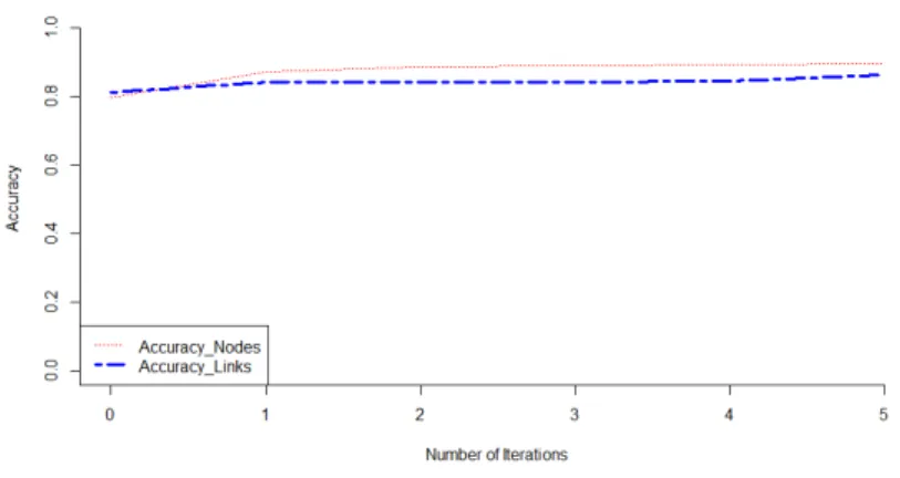
Figure 2: LFR: corrected nodes and links: case of 30 noisy nodes and 50 noisy links.
In these experiments we will limit ourselves to 5 iterations since beyond this number, the variation of the accuracy becomes negligible.
385
In order to show the convergence of our evidential approach, we will consider an LFR network composed of 99 nodes, 191 links and 3 communities. We will noise 30 nodes and 50 links and evaluate the behavior of the proposed algorithm. Figure 2 shows the evolution of the accuracy from an iteration to another. We took the case of 30 noisy nodes and 50 noisy links (Evidential Attributes).
390
We can notice that from an iteration to another, the accuracy value increases which means that the algorithm succeeds in correcting the noise.
4.4. Baseline
In order to show the efficiency of our method, we have performed an algo-rithm that uses the same principle in probabilistic version.
395
Step 1: Generation of Probabilities
In this step, we generate randomly N values in [0, 1] for each node and N + 1 probabilities for each link then we normalize. We generate N + 1 probalities as we have ICi links within communities and BC links that connect communities to each other. Then, we associate the maximum probability generated with the
400
as follow:
• (p(C1), p(C2), . . . , p(CN)) for each node.
• (p(IC1), p(IC2), p(IC3), . . . , p(ICN), p(BC)) for each link. Step 2: Calculation of Distances
405
In this step, we will calculate the Euclidean distances between the attributes of each node/link composing a triplet with those of the representatives of each group:
• For the nodes: certain events are defined by pΩN
ω (ω) = 1 with ω ∈ ΩN i.e. pΩN
Ci (Ci) = 1, with i = {1, . . . , N }. 410
• For the links: certain events are defined by pΩL
ω (ω) = 1 with ω ∈ ΩL i.e. pΩL
BC(BC) = 1 or p ΩL
ICi(ICi) = 1 , with i = {1, . . . , N }.
Depending of the number of communities composing the network, every representative will have 1 on the attribute of its class and 0 on the others. For example, if we consider a representative of C1 and we have 3 communities in
415
the network, its probabilities vector will be R1= (1, 0, 0). Hence, we have: Ck1 = arg min ω∈ΩN dE(pΩk1N, p ΩN ω ) (21) Ck2 = arg min ω∈ΩN dE(pΩN k2 , p ΩN ω ) (22)
Lk12 is determined according to the coherent triplets by:
Lk12= ICk1 if Ck1 = Ck2 BC if Ck1 6= Ck2 (23)
Step 3: Calculation of Average Distances
In this step, we will calculate the minimal average distance of each triplet k defined by: dk = dE(pΩN k1, p ΩN Ck1) + dE(p ΩL k12, p ΩL Lk12) + dE(p ΩN k2 , p ΩN Ck2) 3 (24)
Step 4: Assignment of probabilities from distances
420
In this step, we will assign the probabilities resulting from the computation of the distances between triplets. We use the values of the minimal average distance dk. Hence, we have: pΩN k1d(Ck1) = 1 − dk pΩN k1d(Ck1) = dk N − 1 (25) pΩL k12d(Lk12) = 1 − dk pΩL k12d(Lk12) = dk N (26) pΩN k2d(Ck2) = 1 − dk pΩN k2d(C t k2) = dk N − 1 (27)
We precise that Ck1, Lk12, Ck2 represent respectively the elements contrary to Ck1, Lk12, Ck2.
425
Step 5: Calculation of the average between the new probabilities and the initial ones
In order to have a single probability distribution for each node/link, we will calculate the average between the probabilities generated in the first instance and those resulting from the calculation of the distances.
430 pt+1,ΩN k1 = pt,ΩN k1 + p t,ΩN k1d 2 (28) pt+1,ΩL k12 = pt,ΩL k12 + p t,ΩL k12d 2 (29) pt+1,ΩN k2 = pt,ΩN k2 + p t,ΩN k2d 2 (30) where pt,ΩN k1d , p t,ΩL k12d, p t,ΩN
k2d are given respectively by equations (25), (26) and (27).
In order to determine a unique probabilities vector for each node (e.g. Vk1),
ob-tained for the given node Vk1. Hence, we have: pΩN k1 = 1 |T | X {k:Vk1∈T } pΩN k (31) where T = {(Vk0 1, Lk12, Vk2)} and p ΩN
k is given by the equation (28).
435
Step 6: Making Decision
In this step, we will decide on the membership of each node/link. To do this, we decide the singleton having the maximum of probability.
Algorithm 2 A Probabilistic Approach for Correcting Noise
Require: Graph G(V, E), The set of labeled nodes, the set of labeled links Ensure: The corrected graph.
t = 0 repeat
1. for each element of a triplet k, compute the Euclidean distance between the element and the corresponding categorical representative using Eqs (21), (22), (23)
2. for each triplet k, compute the minimum average distance dk by using Eq (24)
3. Define probabilities from the computed dk using the Eqs (25), (26), (27)
4. Update the probabilities using the Eqs (28),(29), (30),
5. Combine the probabilities for the same node in order to have a unique vector of probabilities by using the Eq (31)
6. Make decision about the belonging of each element of the triplet k 7. t = t + 1
until Number of iterations equal to 5.
Algorithm 2 shows the outline of the process followed for correcting noise in social network using probabilistic attributes.
440
In order to test the effectiveness of the baseline, we will add the noise as we did with the evidential approach. To do this, we will add noise to the same
Noise Rate of improvement 30 Nodes 60%
60 Nodes 53% 90 Nodes 42% 99 Nodes 38%
Table 2: Improvement Rate: Case of Noisy Nodes Only.
Noise Rate of improvement 50 Links 41%
100 Links 36.7% 191 Links 36%
Table 3: Improvement Rate: Case of Noisy Links Only.
nodes and links selected randomly when we tested the evidential approach.
4.5. Improvement Rate
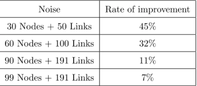
Tables 2, 3, 4, 5 show the rate of improvement of the evidential approach
445
compared to the baseline at the fifth iteration. We consider the variation of noise in the LFR network composed of 99 nodes, 191 links and 3 communities. The rate of improvement is calculated by making the difference between the average values of the accuracy obtained with the evidential approach at the fifth iteration with that given by the baseline.
450
Noise Rate of improvement 30 Nodes + 50 Links 45%
60 Nodes + 100 Links 32% 90 Nodes + 191 Links 11% 99 Nodes + 191 Links 7%
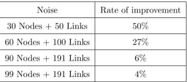
Noise Rate of improvement 30 Nodes + 50 Links 50%
60 Nodes + 100 Links 27% 90 Nodes + 191 Links 6% 99 Nodes + 191 Links 4%
Table 5: Improvement Rate for Links: Case of Noisy Nodes and Noisy Links.
4.6. Experiments on Real Data: Karate Club
As the karate club network has 2 communities, the frames of discernment of the nodes and links will be defined by:
• ΩN = {C1, C2} • ΩL= {IC1, IC2, BC}
455
In this part, we will show the results obtained in the case of noisy nodes only, noisy links only and noisy nodes and links at the same time.
4.6.1. Noisy Nodes Only
In figure 3 we present the accuracy average values at the fifth iteration when we vary the number of noisy nodes.
460
We notice that the more the number of noisy nodes increases, the more the accuracy average value decreases for both evidential and probabilistic methods. However, we remark that we obtain a better accuracy average results with the belief function theory comparing to the probability theory. This can be explained by the fact that the theory of belief functions manages ignorance as
465
well as conflict.
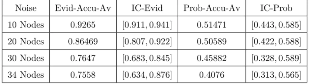
Table6 presents the accuracy averages and the confidence intervals obtained from the evidential approach and the baseline for each level of noise added to the nodes only in the case of the Karate Club.
Figure 3: Karate Club: comparison of probabilistic and evidential accuracy: case of noisy nodes.
Noise Evid-Accu-Av IC-Evid Prob-Accu-Av IC-Prob 10 Nodes 0.9265 [0.911, 0.941] 0.51471 [0.443, 0.585] 20 Nodes 0.86469 [0.807, 0.922] 0.50589 [0.422, 0.588] 30 Nodes 0.7647 [0.683, 0.845] 0.45882 [0.328, 0.589] 34 Nodes 0.7558 [0.634, 0.876] 0.4076 [0.313, 0.565]
Table 6: Accuracy Average and Interval of Confidence: Case of Noisy Nodes Only in the Karate Club.
4.6.2. Noisy Links Only
470
We show in figure 4 the accuracy average results at the fifth iteration after noising 20, 40, 60 and 78 links of the network.
According to the curve, the average accuracy values given by the evidential approach are better than that given by the baseline in each level of noise.
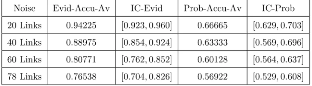
We show in table7 the obtained accuracy averages and the confidence
in-475
tervals given by the evidential method and the probabilistic approach when we vary the number of noisy links only in the case of the Karate Club.
Figure 4: Karate Club: comparison of probabilistic and evidential accuracy: case of noisy links.
Noise Evid-Accu-Av IC-Evid Prob-Accu-Av IC-Prob 20 Links 0.94225 [0.923, 0.960] 0.66665 [0.629, 0.703] 40 Links 0.88975 [0.854, 0.924] 0.63333 [0.569, 0.696] 60 Links 0.80771 [0.762, 0.852] 0.60128 [0.564, 0.637] 78 Links 0.76538 [0.704, 0.826] 0.56922 [0.529, 0.608]
Table 7: Accuracy Average and Interval of Confidence: Case of Noisy Links Only in the Karate Club.
4.6.3. Noisy Nodes and Noisy Links
In this third case, we proceed by noising the nodes and the links at the same time. Figure 5 shows the obtained results of accuracy average after noising the
480
attributes at the fifth iteration. The abscissa represents respectively the level of noise 10 nodes and 20 links, 20 nodes and 40 links, 30 nodes and 60 links and finally, 34 nodes and 78 links.
We notice that the accuracy average values decreases as the noise level in-creases for both evidential and probabilistic approaches. However, the proposed
485
method gives better results than the baseline.
Figure 5: Karate Club: comparison of probabilistic and evidential accuracy: case of noisy nodes and links.
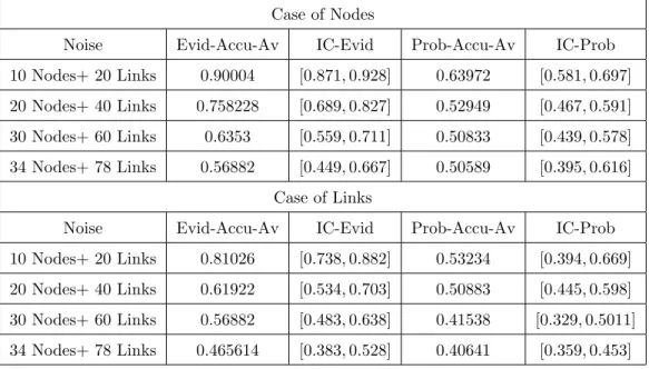
given by the evidential method and the probabilistic approach in the case of noisy nodes and noisy links in the case of the Karate Club.
4.7. Experiments on LFR
490
In the second part of our experiments, we used different networks generated with LFR [26]. We present in table 9 the parameters used to generate our networks.
We will perform several experimentations which will be repeated 10 times and show the obtained average of the accuracy. All the figures present the
495
results given by the evidential approach and the baseline.
We will start by varying the noise of the nodes, links and both of the LFR network composed of 99 nodes, 191 links and 3 communities.
For the rest of the experiments, we will vary each time one of the parameters of the LFR network such as the number of communities, the size of the network
500
and the mixing parameter µ and observe their impact on the noise correction rate. For each of these experiments we will noise 60% of the nodes and 50% of the links.
Case of Nodes
Noise Evid-Accu-Av IC-Evid Prob-Accu-Av IC-Prob 10 Nodes+ 20 Links 0.90004 [0.871, 0.928] 0.63972 [0.581, 0.697] 20 Nodes+ 40 Links 0.758228 [0.689, 0.827] 0.52949 [0.467, 0.591] 30 Nodes+ 60 Links 0.6353 [0.559, 0.711] 0.50833 [0.439, 0.578] 34 Nodes+ 78 Links 0.56882 [0.449, 0.667] 0.50589 [0.395, 0.616]
Case of Links
Noise Evid-Accu-Av IC-Evid Prob-Accu-Av IC-Prob 10 Nodes+ 20 Links 0.81026 [0.738, 0.882] 0.53234 [0.394, 0.669] 20 Nodes+ 40 Links 0.61922 [0.534, 0.703] 0.50883 [0.445, 0.598] 30 Nodes+ 60 Links 0.56882 [0.483, 0.638] 0.41538 [0.329, 0.5011] 34 Nodes+ 78 Links 0.465614 [0.383, 0.528] 0.40641 [0.359, 0.453]
Table 8: Accuracy Average and Interval of Confidence: Case of Noisy Nodes and Links in the Karate Club.
generation of our networks: n represents the number of nodes, K the average
505
degree, maxK the maximum degree, mu the mixing parameter, t1 the minus exponent for the degree sequence, t2 the minus exponent for the community size distribution, minC the minimum for the community size, maxC the maximum for the community size, on the number of overlapping nodes, om the number of memberships of the overlapping nodes and C the average clustering coefficient.
510
Since LFR generates the links of the graph in both directions and in this work we consider non-directed graphs, we will use a single link to represent the connection between two nodes. As a result, the number of links we present in the experimental part is half the number of links initially generated.
The first set of experiments consists of varying the noise in an LFR network
515
composed of 99 nodes, 191 links and 3 communities. We will proceed by noising the nodes at first, then the links and finally we will simultaneously noise both. The frames of discernment of the nodes and links for this network are defined as follows:
N K maxK mu t1 t2 minC maxC on om C 99 5 10 0.3 2 1 33 33 0 0 0.55 200 5 10 0.3 2 1 66 67 0 0 0.55 200 5 10 0.3 2 1 50 50 0 0 0.55 200 5 10 0.3 2 1 40 40 0 0 0.55 200 5 10 0.3 2 1 33 33 0 0 0.55 300 5 10 0.3 2 1 100 100 0 0 0.55 400 5 10 0.3 2 1 132 135 0 0 0.55 50 5 10 0.3 2 1 15 17 0 0 0.55 200 5 10 0.1 2 1 66 67 0 0 0.55 200 5 10 0.5 2 1 66 67 0 0 0.55 200 5 10 0.7 2 1 66 67 0 0 0.55 200 5 10 0.9 2 1 66 67 0 0 0.55 Table 9: Parameters of LFR • ΩN = {C1, C2, C3} 520
• ΩL = {IC1, IC2, IC3, BC} with ICi represents the links inside the com-munity Ci and BC represents the links between 3 communities.
4.7.1. Noisy Nodes Only
In this first case of experiments, we will add noise to a number of nodes randomly selected of the network. The noise consists on modifying the mass
525
functions of the selected nodes by randomly generating two focal elements (ig-norance and another element except the empty set). We will then compare the obtained results with those given by the baseline. Figure 6 shows the obtained results of the accuracy for every variation of the noise. We vary the number of noisy nodes from 30 to 99.
530
We notice that the more the number of noisy nodes increases the more the accuracy average decreases. We also note that for each level of noise, we obtained better results with the evidential model. This is because the theory of belief
Figure 6: LFR: comparison of probabilistic and evidential accuracy: case of noisy nodes.
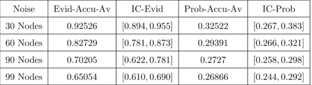
Noise Evid-Accu-Av IC-Evid Prob-Accu-Av IC-Prob 30 Nodes 0.92526 [0.894, 0.955] 0.32522 [0.267, 0.383] 60 Nodes 0.82729 [0.781, 0.873] 0.29391 [0.266, 0.321] 90 Nodes 0.70205 [0.622, 0.781] 0.2727 [0.258, 0.298] 99 Nodes 0.65054 [0.610, 0.690] 0.26866 [0.244, 0.292]
Table 10: Accuracy Average and Interval of Confidence: Case of Noisy Nodes Only in LFR.
functions offers a very effective way to handle ignorance and conflict.
Table10 shows the obtained accuracy averages and the confidence intervals
535
given by the evidential method and the probabilistic approach in the case of noisy nodes only in the case of LFR network.
4.7.2. Noisy Links Only
The second part of the experiments consists in keeping the initial generation of the mass functions of the nodes and adding noise only to the mass functions
540
of the links.
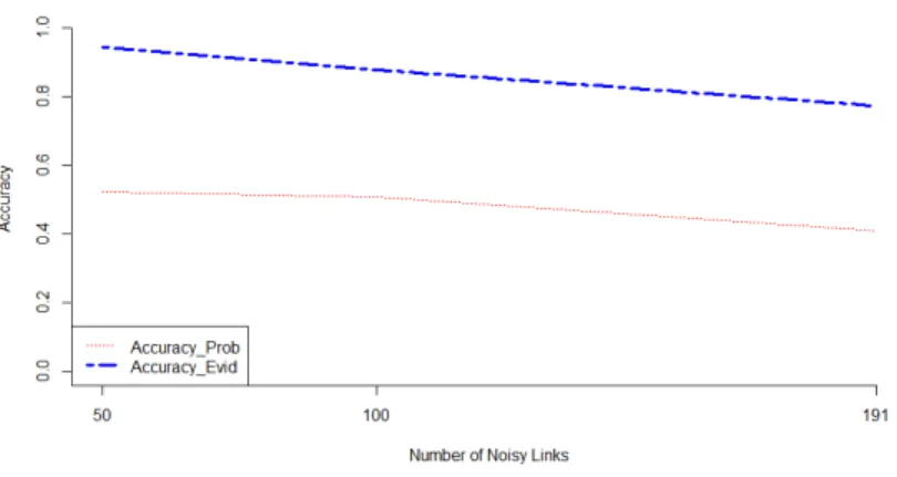
Figure 7 shows the obtained results of the accuracy average due to the vari-ation in the number of noisy links. In this figure, we compute the accuracy average for 50, 100 and 191 noisy links. We notice that we obtain better results
Figure 7: LFR: comparison of probabilistic and evidential accuracy: case of noisy links.
Noise Evid-Accu-Av IC-Evid Prob-Accu-Av IC-Prob 50 Links 0.94239 [0.930, 0.953] 0.52252 [0.474, 0.570] 100 Links 0.87539 [0.862, 0.887] 0.50786 [0.458, 0.557] 191 Links 0.77119 [0.739, 0.803] 0.40988 [0.352, 0.467]
Table 11: Accuracy Average and Interval of Confidence: Case of Noisy Links Only in LFR.
when we use the evidential attributes. These results can be explained by the
545
fact that the evidential approach better manages ignorance than the probabilis-tic approach.
We present in table11 the accuracy averages and the confidence intervals obtained from the evidential approach and the baseline in the case of noisy links only in the case of LFR network.
550
4.7.3. Noisy Nodes and Noisy Links
In this third part of the experiments, we noised simultaneously the nodes and the links of the network.
The aim of simultaneously noising the nodes and the links is to make the network totally incoherent and to evaluate the ability of the algorithms to correct
555
Figure 8: LFR: comparison of probabilistic and evidential accuracy: case of noisy nodes and links.
We vary the number of noisy nodes by 30 at each step and then we add noise on all the nodes of the network. As for the links, we vary the noisy links by 50, then we add noise on all the links of the network.
We chose these values in order to have a better view on the impact of the
560
noise introduced on the network information.
We compare the obtained results with those of the baseline.
Figure 8 shows the results of the accuracy average for every level of noise used in these experiments. We compare the obtained results with those of the baseline after noising 30 nodes and 50 links, 60 nodes and 100 links, 90 nodes
565
and 191 links and finally, 99 nodes and 191 links.
From this figure, we can notice that the accuracy average results are better with the evidential attributes. We remark also that when it is very noisy, it becomes impossible to obtain good results.
It should be noted that in the case of adding a maximum noise, the value
570
of the accuracy average is stable from the beginning. This is due to the fact that when we noise the data, the mass functions are generated randomly and therefore there are two possibilities:
Case of Nodes
Noise Evid-Accu-Av IC-Evid Prob-Accu-Av IC-Prob 30 Nodes+ 50 Links 0.9091 [0.882, 0.936] 0.45125 [0.390, 0.511] 60 Nodes+ 100 Links 0.71417 [0.664, 0.763] 0.3901 [0.311, 0.412] 90 Nodes+ 191 Links 0.40602 [0.367, 0.444] 0.29088 [0.245, 0.325] 99 Nodes+ 191 Links 0.34643 [0.293, 0.399] 0.27016 [0.227, 0.312]
Case of Links
Noise Evid-Accu-Av IC-Evid Prob-Accu-Av IC-Prob 30 Nodes+ 50 Links 0.84188 [0.810, 0.872] 0.3333 [0.266, 0.399] 60 Nodes+ 100 Links 0.59634 [0.558, 0.633] 0.3232 [0.262, 0.383] 90 Nodes+ 191 Links 0.3434 [0.313, 0.398] 0.27436 [0.247, 0.305] 99 Nodes+ 191 Links 0.2929 [0.258, 0.312] 0.24987 [0.228, 0.275]
Table 12: Accuracy Average and Interval of Confidence: Case of Noisy Nodes and Noisy Links in LFR.
• Either the element always retains its initial membership but with a
differ-575
ent mass function.
Hence, we will always have elements that are correct even when it’s the case of maximal noise. These correct attributes help in the finding of other correct triplets.
We present in table12 a comparison between the accuracy averages and the
580
confidence intervals given by the evidential approach and the baseline in the case of noisy nodes and noisy links in the case of LFR network.
In what follows, we will noise 60% of nodes and 50% of links by varying each time a parameter of the LFR algorithm. The idea is to see the impact of each parameter on the correction rate of noisy information for the same level of
585
noise. To do this, we will first vary the number of communities. Then, we will vary the n which represents the number of nodes composing the network and finally, we will vary the mixing parameter.
Figure 9: LFR: comparison of probabilistic and evidential accuracy: case of noisy nodes and links.
4.8. LFR: Variation of the Communities number
In this part of experiments, we vary the number of communities. We generate
590
4 LFR networks:
• a network with 200 nodes, 402 links and 3 communities. • a network with 200 nodes, 472 links and 4 communities. • a network with 200 nodes, 477 links and 5 communities. • a network with 200 nodes, 501 links and 6 communities.
595
Figure 9 shows the obtained results of the accuracy average for each network. We can remark that for all the networks, the evidential model gives better results on links and nodes accuracy average than the baseline. We notice also that there is not really a big difference in the values of the accuracy average when we vary the number of communities. We can, therefore, conclude that the proposed
600
approach is stable.
Table13 presents a comparison between the accuracy averages and the confi-dence intervals given by the evidential approach and the probabilistic one when we vary the number of communities in the case of LFR networks.
Case of Nodes
Nb-Communities Evid-Accu-Av IC-Evid Prob-Accu-Av IC-Prob C3 0.73 [0.689, 0.774] 0.39 [0.321, 0.402] C4 0.625 [0.602, 0.645] 0.32 [0.281, 0.345] C5 0.65 [0.63, 0.679] 0.41 [0.385, 0.445] C6 0.6 [0.598, 0.621] 0.38 [0.365, 0.4]
Case of Links
Nb-Communities Evid-Accu-Av IC-Evid Prob-Accu-Av IC-Prob C3 0.61 [0.563, 0.669] 0.30 [0.298, 0.325] C4 0.553 [0.524, 0.573] 0.2247 [0.201, 0.251] C5 0.6065 [0.575, 0.613] 0.3939 [0.371, 0.405] C6 0.53 [0.508, 0.554] 0.33 [0.295, 0.353]
Table 13: Accuracy Average and Interval of Confidence: Case of Noisy Nodes and Noisy Links-Communities Variation.
4.9. LFR: Variation of the Size of the Network
605
In this section, we will present the obtained results of the accuracy following the variation of the network size. We consider 5 networks whose number of nodes was varied and containing 3 communities:
• a network with 50 nodes and 115 links. • a network with 99 nodes and 191 links.
610
• a network with 200 nodes and 402 links. • a network with 300 nodes and 721 links. • a network with 400 nodes and 932 links.
Figure 10 presents the obtained accuracy average results. It shows that the evidential approach was able to correct more information than the baseline
615
Figure 10: LFR: comparison of probabilistic and evidential accuracy: case of variation of the size of the network.
method is stable since the values of the precision calculated for each network are close to each other.
Table14 shows the obtained accuracy averages and the confidence intervals from the evidential approach and the probabilistic one when we vary the size of
620
the network in the case of LFR.
4.10. LFR: Variation of the Mixing Parameter µ
In this section, we will present the obtained results of the accuracy average following the variation of the mixing parameter µ. We consider 5 networks whose mixing parameter was varied and containing 3 communities:
625
• a network with 200 nodes, 484 links and µ = 0.1. • a network with 200 nodes, and 402 links and µ = 0.3. • a network with 200 nodes, and 467 links and µ = 0.5. • a network with 200 nodes, and 488 links and µ = 0.7. • a network with 200 nodes, and 502 links and µ = 0.9.
Case of Nodes
Nb-Nodes Evid-Accu-Av IC-Evid Prob-Accu-Av IC-Prob 50 0.77 [0.705, 0.798] 0.44 [0.365, 0.463] 99 0.71417 [0.664, 0.763] 0.3901 [0.311, 0.412] 200 0.73 [0.698, 0.773] 0.39 [0.321, 0.402] 300 0.69 [0.602, 0.725] 0.38 [0.309, 0.395] 400 0.68 [0.598, 0.699] 0.37 [0.312, 0.385] Case of Links
Nb-Nodes Evid-Accu-Av IC-Evid Prob-Accu-Av IC-Prob 50 0.65 [0.585, 0.705] 0.37 [0.303, 0.398] 99 0.59634 [0.558, 0.633] 0.3232 [0.315, 0.3434] 200 0.61 [0.563, 0.669] 0.30 [0.298, 0.325] 300 0.58 [0.538, 0.621] 0.29 [0.205, 0.382] 400 0.57 [0.545, 0.611] 0.27 [0.203, 0.351]
Table 14: Accuracy Average and Interval of Confidence: Case of Noisy Nodes and Noisy Links-Network Size Variation.
Figure 11: LFR: comparison of probabilistic and evidential accuracy: case of variation of the mixing parameter.
Figure 11 shows the results obtained by the evidential method and the base-line after varying the mixing parameter.
We find that the accuracy average of the nodes is greater than the accuracy average of the links when µ < 0.5, while the latter becomes greater than the accuracy average of the nodes when µ > 0.5. This change is explained by
635
the fact that the more the mixing parameter approaches 1, the more we get a network with more links between clusters than within the community.
We present in table15 the obtained accuracy averages and the confidence intervals given by the evidential approach and the baseline when we vary the mixing parameter in the case of LFR.
640
4.11. Comparison of execution time
In this section, we will compare the execution time put by the model’s ev-idential version as well as the probabilistic one. We will present the execution time at the fifth iteration. We will observe the evolution of the execution time in the case of LFR networks with 6, 5, 4 and 3 communities. The execution
645
time will be expressed in seconds.
Case of Nodes
µ Evid-Accu-Av IC-Evid Prob-Accu-Av IC-Prob 0.1 0.732 [0.689, 0.774] 0.42346 [0.394, 0.452] 0.3 0.73 [0.687, 0.773] 0.39 [0.321, 0.402] 0.5 0.6625 [0.626, 0.698] 0.325 [0.291, 0.358] 0.7 0.645 [0.604, 0.685] 0.19939 [0.181, 0.217] 0.9 0.6315 [0.602, 0.658] 0.16455 [0.143, 0.185] Case of Links
µ Evid-Accu-Av IC-Evid Prob-Accu-Av IC-Prob 0.1 0.60426 [0.564, 0.644] 0.3255 [0.273, 0.377] 0.3 0.61 [0.563, 0.669] 0.30 [0.298, 0.325] 0.5 0.67687 [0.626, 0.698] 0.25868 [0.239, 0.277] 0.7 0.711 [0.690, 0.732] 0.3425 [0.320, 0.364] 0.9 0.75238 [0.741, 0.763] 0.3545 [0.3283, 0.380]
Table 15: Accuracy Average and Interval of Confidence: Case of Noisy Nodes and Noisy Links-Mixing Parameter Variation.
C3 C4 C5 C6
Probabilistic Execution Time 5.45 8.1 8.95 9.45 Evidential Execution Time 119.05 652.4 3864.15 19225.4
to the baseline. We notice also that as the number of communities increases, the execution time increases too.
We remind that in this paper, we focused on the use of a limited number
650
of communities. In terms of scaling up, there are several strategies that can reduce complexity such as representing only the focal elements or grouping them together if their values are negligible. This will be the subject of future work.
5. Conclusion
655
Researches that have focused on clustering using the network structure as well as the nodes attributes, ignore the links information. In order to remedy this problem, we propose a method which allows to classify the nodes in their initial clusters even when there is a significant noise added to the network. In the case of a large noise, the algorithm guarantees the information coherence of
660
any network even when it is a network whose nodes and links attributes have been strongly modified.
Throughout this work, we first recalled some basic notions of the theory of belief functions as well as some methods for the communities detection based on graph structure as well as the attributes and some other related works. Then,
665
we presented our method which consists in first generating attributes on the nodes and the links according to the network structure. In a second step, we added noise on the attributes and then reclassified the nodes and/or the links.
We tested our approach on real data: the Karate Club network. Then, we varied the noise on a LFR network composed of 3 communities and we presented
670
the obtained results during the noising of the nodes, links and both. Finally, we studied the behavior of the proposed method according to the variation of the number of communities, the size of the network as well as the mixing parameter. All the obtained results were compared with those of the baseline. Experiments have shown that the more we noisy the network, the farther we get away from
675
our proposed approach is stable when we vary the number of communities and the size of the network and gives better results in all studied cases than the baseline.
As future work, we intend to deal with the case of overlapping communities.
680
Given the fact that a node can belong to several communities, it has become interesting to analyze the evolution of a social network over time. This study could help to better identify the types of nodes as well as their exchanges on the network. In addition, the theory of belief function offers a very effective way to analyze the evolution during the time of evidential networks composed
685
of overlapping communities.
We also intend to improve the code and the execution time of the proposed method. In fact, although the proposed approach yields better results, it takes much longer time than the baseline.
References
690
[1] S. Wasserman, K. Faust, Social network analysis: Methods and applica-tions, Vol. 8, Cambridge university press, 1994.
[2] C. Prell, Social network analysis: History, theory and methodology, Sage, 2012.
[3] S. Fortunato, Community detection in graphs, Physics reports 486 (3)
695
(2010) 75–174.
[4] E. Adar, C. Re, Managing uncertainty in social networks., IEEE Data Eng. Bull. 30 (2) (2007) 15–22.
[5] S. Ben Dhaou, M. Kharoune, A. Martin, B. B. Yaghlane, Belief approach for social networks, in: International Conference on Belief Functions, Springer,
700
2014, pp. 115–123.
[6] S. Ben Dhaou, K. Zhou, M. Kharoune, A. Martin, B. Ben Yaghlane, The advantage of evidential attributes in social networks, in: Information Fusion (Fusion), 2017 20th International Conference on, IEEE, 2017, pp. 1–8.
[7] G. Shafer, A mathematical theory of evidence, Vol. 1, Princeton university
705
press Princeton, 1976.
[8] T. Denœux, A k-nearest neighbor classification rule based on dempster-shafer theory, Classic works of the Dempster-Shafer theory of belief func-tions (2008) 737–760.
[9] Z.-G. Liu, Q. Pan, G. Mercier, J. Dezert, A new incomplete pattern
clas-710
sification method based on evidential reasoning, IEEE transactions on cy-bernetics 45 (4) (2015) 635–646.
[10] D. Wei, X. Deng, X. Zhang, Y. Deng, S. Mahadevan, Identifying influential nodes in weighted networks based on evidence theory, Physica A: Statistical Mechanics and its Applications 392 (10) (2013) 2564–2575.
715
[11] A. Martin, Implementing general belief function framework with a practical codification for low complexity, Advances and applications of DSmT for Information Fusion-Collected works 3 (2009) 217–273.
[12] G. Shafer, Perspectives on the theory and practice of belief functions, In-ternational Journal of Approximate Reasoning 4 (5-6) (1990) 323–362.
720
[13] A.-L. Jousselme, D. Grenier, ´E. Boss´e, A new distance between two bodies of evidence, Information fusion 2 (2) (2001) 91–101.
[14] G. Shafer, Dempster’s rule of combination, International Journal of Ap-proximate Reasoning 79 (2016) 26–40.
[15] P. Smets, Decision making in the tbm: the necessity of the pignistic
trans-725
formation, International Journal of Approximate Reasoning 38 (2) (2005) 133–148.
[16] D. S. Seong, H. S. Kim, K. H. Park, Incremental clustering of attributed graphs, IEEE transactions on systems, man, and cybernetics 23 (5) (1993) 1399–1411.
[17] Y. Zhou, H. Cheng, J. X. Yu, Graph clustering based on struc-tural/attribute similarities, Proceedings of the VLDB Endowment 2 (1) (2009) 718–729.
[18] J. Leskovec, J. J. Mcauley, Learning to discover social circles in ego net-works, in: Advances in neural information processing systems, 2012, pp.
735
539–547.
[19] A. Trabelsi, Z. Elouedi, E. Lefevre, Handling uncertain attribute values in decision tree classifier using the belief function theory, in: International Conference on Artificial Intelligence: Methodology, Systems, and Applica-tions, Springer, 2016, pp. 26–35.
740
[20] K. Zhou, A. Martin, Q. Pan, Z. Liu, Selp: Semi-supervised evidential label propagation algorithm for graph data clustering, International Journal of Approximate Reasoning 92 (2018) 139–154.
[21] R. Guimer`a, M. Sales-Pardo, Missing and spurious interactions and the reconstruction of complex networks, Proceedings of the National Academy
745
of Sciences 106 (52) (2009) 22073–22078.
[22] N. Vuokko, E. Terzi, Reconstructing randomized social networks, in: Pro-ceedings of the 2010 SIAM International Conference on Data Mining, SIAM, 2010, pp. 49–59.
[23] A. Essaid, A. Martin, G. Smits, B. Ben Yaghlane, A Distance-Based
De-750
cision in the Credal Level, in: International Conference on Artificial Intel-ligence and Symbolic Computation (AISC 2014), Sevilla, Spain, 2014, pp. 147 – 156.
[24] The uci network data repository.
URL http://networkdata.ics.uci.edu/index.php.
755
[25] A. Lancichinetti, S. Fortunato, F. Radicchi, Benchmark graphs for testing community detection algorithms, Physical review E 78 (4) (2008) 046110.
[26] Lancichinetti-fortunato-radicchi benchmark.
URL https://figshare.com/articles/Lancichinetti_Fortunato_ Radicchi_LFR_benchmark/1149962


![[PDF] Cours Principes des langage de programmation Caml | Formation informatique](data:image/gif;base64,R0lGODlhAQABAIAAAP///wAAACH5BAEAAAAALAAAAAABAAEAAAICRAEAOw==)